
Recent posts have stressed the complexity of climates and their component variables. However, global warming was invented on the back of a single metric: rising global mean temperatures the last decades of last century. That was de-emphasized during the “pause” but re-emerged lately with the El-Nino-induced warming. So this post is focusing on that narrow aspect of climate change.
There are several papers on this blog referring to a quasi-60 year oscillation of surface temperatures due to oceanic circulations. I have also noted the attempts by many to make the link between solar activity (SA) and earth climate patterns.
Dan Pangburn is a professional engineer who has synthesized the solar and oceanic factors into a mathematical model that correlates with Average Global Temperature (AGT). On his blog is posted a monograph (here) Cause of Global Climate Change explaining clearly his thinking and the maths. I am providing some excerpts and graphs as a synopsis of his analysis, in hopes others will also access and appreciate his work on this issue.
Introduction
The basis for assessment of AGT is the first law of thermodynamics, conservation of energy, applied to the entire planet as a single entity. Much of the available data are forcings or proxies for forcings which must be integrated (mathematically as in calculus, i.e. accumulated over time) to compute energy change. Energy change divided by effective thermal capacitance is temperature change. Temperature change is expressed as anomalies which are the differences between annual averages of measured temperatures and some baseline reference temperature; usually the average over a previous multiple year time period. (Monthly anomalies, which are not used here, are referenced to previous average for the same month to account for seasonal norms.)
At this point, it appears reasonable to consider two temperature anomaly data sets extending through 2015. These are co-plotted on Figure 8.

1) The set used previously [12] through 2012 with extension 2013-2015 set at the average 2002-2012 (when the trend was flat) at 0.4864 K above the reference temperature. 2) Current (5/27/16) HadCRUT4 data set [13] through 2012 with 2013-2015 set at the average 2002-2012 at 0.4863 K above the reference temperature.
Oceanic Climate Impacts
Approximation of the sea surface temperature anomaly oscillation can be described as varying linearly from –A/2 K in 1909 to approximately +A/2 K in 1941 and linearly back to the 1909 value in 1973. This cycle repeats before and after with a period of 64 years.

Figure 1: Ocean surface temperature oscillations (α-trend) do not significantly affect the bulk energy of the planet.
Comparison with PDO, ENSO and AMO
Ocean cycles are perceived to contribute to AGT in two ways: The first is the direct measurement of sea surface temperature (SST). The second is warmer SST increases atmospheric water vapor which acts as a forcing and therefore has a time-integral effect on temperature. The approximation, (A,y), accounts for both ways.
Successful accounting for oscillations is achieved for PDO and ENSO when considering these as forcings (with appropriate proxy factors) instead of direct measurements. As forcings, their influence accumulates with time. The proxy factors must be determined separately for each forcing.

Figure 2: Comparison of idealized approximation of ocean cycle effect and the calculated effect from PDO and ENSO.
The AMO index [9] is formed from area-weighted and de-trended SST data. It is shown with two different amounts of smoothing in Figure 3 along with the saw-tooth approximation for the entire planet per Equation (2) with A = 0.36.

The high coefficients of determination in Table 1 and the comparisons in Figures 2 and 3 corroborate the assumption that the saw-tooth profile with a period of 64 years provides adequate approximation of the net effect of all named and unnamed ocean cycles in the calculated AGT anomalies.
Solar-Climate Connection
An assessment of this is that sunspots are somehow related to the net energy retained by the planet, as indicated by changes to average global temperature. Fewer sunspots are associated with cooling, and more sunspots are associated with warming. Thus the hypothesis is made that SSN are proxies for the rate at which the planet accumulates (or loses) radiant energy over time. Therefore the time-integral of the SSN anomalies is a proxy for the amount of energy retained by the planet above or below breakeven.
Also, a lower solar cycle over a longer period might result in the same increase in energy retained by the planet as a higher solar cycle over a shorter period. Both magnitude and time are accounted for by taking the time-integral of the SSN anomalies, which is simply the sum of annual mean SSN (each minus Savg) over the period of study.
The values for Savg are subject to two constraints. Initially they are determined as that which results in derived coefficients and maximum R2. However, calculated values must also result in rational values for calculated AGT at the depths of the Little Ice Age. The necessity to calculate a rational LIA AGT is a somewhat more sensitive constraint. The selected values for Savg result in calculated LIA AGT of approximately 1 K less than the recent trend which appears rational and is consistent with most LIA AGT assessments.
The sunspot number anomaly time-integral is a proxy for a primary driver of the temperature anomaly β-trend. By definition, energy change divided by effective thermal capacitance is temperature change.

Figure 10: 5-year running average of measured temperatures with calculated prior and future trends (Data Set 1) using 34 as the average daily sunspot number and with V1 SSN. R2 = 0.978887
Projections until 2020 use the expected sunspot number trend for the remainder of solar cycle 24 as provided [6] by NASA. After 2020 the ‘limiting cases’ are either assuming sunspots like from 1924 to 1940 or for the case of no sunspots which is similar to the Maunder Minimum.
Some noteworthy volcanoes and the year they occurred are also shown on Figure 9. No consistent AGT response is observed to be associated with these. Any global temperature perturbation that might have been caused by volcanoes of this size is lost in the natural fluctuation of measured temperatures.
Although the connection between AGT and the sunspot number anomaly time-integral is demonstrated, the mechanism by which this takes place remains somewhat speculative.
Various papers have been written that indicate how the solar magnetic field associated with sunspots can influence climate on earth. These papers posit that decreased sunspots are associated with decreased solar magnetic field which decreases the deflection of and therefore increases the flow of galactic cosmic rays on earth.
These papers [14,15] associated the increased low-altitude clouds with increased albedo leading to lower temperatures. Increased low altitude clouds would also result in lower average cloud altitude and therefore higher average cloud temperature. Although clouds are commonly acknowledged to increase albedo, they also radiate energy to space so increasing their temperature increases S-B radiation to space which would cause the planet to cool. Increased albedo reduces the energy received by the planet and increased radiation to space reduces the energy of the planet. Thus the two effects work together to change the AGT of the planet.
Summary
Simple analyses [17] indicate that either an increase of approximately 186 meters in average cloud altitude or a decrease of average albedo from 0.3 to the very slightly reduced value of 0.2928 would account for all of the 20th century increase in AGT of 0.74 K. Because the cloud effects work together and part of the temperature change is due to ocean oscillation (low in 1901, 0.2114 higher in 2000), substantially less cloud change would suffice.
All of this leaves little warming left to attribute to rising CO2. Pangburn estimates CO2 forcing could be at most 18.6% or 0.23C added since 1895. Given uncertainties in proxies from the past, the estimate could be as low as 0.05C, and the correlation with natural factors would still be .97 R2.
However, all is not lost for CO2. It is still an important player in the atmosphere, despite its impotence as a warming agent.


Reblogged this on TheFlippinTruth.
LikeLike
Reblogged this on Climate Collections.
LikeLike
Reblogged this on 4timesayear's Blog.
LikeLike
Good job, it is a nice clean and simple argument.
LikeLike
Did anyone besides me notice that the ocean temps are predicted to bottom at the same time as solar minimum is predicted to reach bottom? about 2035.
LikeLike
Good catch, Scott. Both the Pacific (PDO) and the Atlantic (AMO) are due for a cooling phase. If that happens coincidental with diminished solar input (indicated by the lower sunspot proxy), we are looking at planetary cooling as suggested by some solar physicists.
The situation reminds of governmental failure in North America to manage the educational system to match demographic shifts. The bureaucratic response comes too late to cope with the current reality. After WWII came the baby boom, and many schools became overcrowded and new ones built. Then the sexual revolution and female liberation produced a baby bust due to smaller families, so schools emptied with surplus capacity. Just as the government got serious about closing schools came the baby echo, unanticipated by the authorities. Despite smaller families, there were many more of therm, these being the married adult boomers. Echo babies were a new pulse of children hitting a school system undergoing downsizing in response to the previous baby bust.
Similarly, the climatists would have us assume endless warming and require cessation of reliable affordable energy just as we enter a mini ice age.
LikeLike
Great work, Ron!
I copied your CO2 table, and updated it for the 2018 CO2 level (408 ppmv), and put it here:
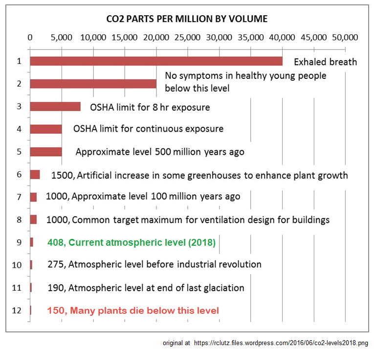
I hope that’s okay with you.
LikeLike
Good job Dave. I have updated the image in the post.
LikeLike
Done, thanks!
(Might need to F5 / refresh to see updated version.)
(Only difference from your new original is the addition of the attribution at the bottom, and also in a metadata comment.)
LikeLike
I take issue with the change to the bottom item. In the original it says “All land plants and animals become extinct below this level”. Land plants become extinct because they are unable to produce fertile seeds. Land animals become extinct because they run out of plants to eat. None of this applies to life in water bodies.
LikeLike
Dan, I changed it because someone pointed out that C3 plants can survive below 150 ppm CO2, and thus some animals could live off the greatly reduced food supply. The point is still made in the edited version that 150 is a dangerous boundary for the biosphere.
https://biology.stackexchange.com/questions/29943/whats-the-or-some-of-the-minimums-amount-of-atmospheric-carbon-dioxide-need
LikeLike
Ron, Thanks for the comment. I agree it is kind of a quibble. My point is/was that without viable seeds, eventually the plants will be gone. Since then I thought about ferns, some of which reproduce without seeds and I have seen no data on whether they can still reproduce below 150 ppmv or not. Certainly your change is OK regardless. As I recall, in the first draft of the graph, I had a similar statement but decided on the stronger one based on a little research (unfortunately I do not have the reference) and not a lot of thought.
LikeLike