McKitrick: New PM Carney Tried for Years to Defund Canada

Mark Carney, governor of the Bank of England (BOE), reacts during a news conference at the United Nations COP21 climate summit at Le Bourget in Paris, France, on Friday, Dec. 4, 2015. Photo by Chris Ratcliffe/Bloomberg

Ross McKitrick writes at National Post Carney to lead Canada after trying for years to defund it.  Excerpts in italics with my bolds and added images.

The soon-to-be prime minister’s plan for net-zero banking
would have devastated the country

Conservative leader Pierre Poilievre is very concerned about financial conflicts of interest that new Liberal leader (and our next prime minister) Mark Carney may be hiding. But I’m far more concerned about the one out in the open: Carney is now supposed to act for the good of the country after lobbying to defund and drive out of existence Canada’s oil and gas companies, steel companies, car companies and any other sector dependent on fossil fuels. He’s done this through the Glasgow Financial Alliance for Net Zero (GFANZ), which he founded in 2021.

Carney is a climate zealot. He may try to fool Canadians into thinking he wants new pipelines, liquified natural gas (LNG) terminals and other hydrocarbon infrastructure, but he doesn’t. Far from it. He wants half the existing ones gone by 2030 and the rest soon after.

He has said so, repeatedly and emphatically. He believes that the world “must achieve about a 50 per cent reduction in emissions by 2030” and “rapidly scale climate solutions to provide cleaner, more affordable, and more reliable replacements for unabated fossil fuels.” (By “unabated” he means usage without full carbon capture, which in practice is virtually all cases.) And since societies don’t seem keen on doing this, Carney created GFANZ to pressure banks, insurance companies and investment firms to cut off financing for recalcitrant firms.

“This transition to net zero requires companies across the whole economy to change behaviors through application of innovative technologies and new ways of doing business” he wrote in 2022 with his GFANZ co-chairs, using bureaucratic euphemisms to make his radical agenda somehow seem normal.

The GFANZ plan they articulated that year put companies into four categories. Those selling green technologies or engaged in work that displaces fossil fuels would be rewarded with financing from member institutions. Those still using fossil fuels, or have investments in others that do, but are committed to being “climate leaders” and have set a path to net-zero, would also still be eligible for financing, as would those that do business with “high-emitting firms” but plan to reach net-zero targets on approved timelines. Companies that own or invest in high-emitting assets, however, would operate under a “managed phaseout” regime and could even be cut off from investment capital.

What are “high-emitting assets”? Carney’s group hasn’t released a complete list, but a June 2022 report listed some examples: coal mines, fossil-fuel power stations, oil fields, gas pipelines, steel mills, ships, cement plants and consumer gasoline-powered vehicles. GFANZ envisions a future in which the finance sector either severs all connections to such assets or puts them under a “managed phaseout” regime, which means exactly what it sounds like.

So when Carney jokingly suggested it won’t matter if his climate plan drives up costs for steel mills because people don’t buy steel, he could have added that there likely won’t be any steel mills before long anyway. If his work as prime minister echoes his work as GFANZ chair, we can expect steel mills to be phased out, along with cars, gas-fired power plants, pipelines, oil wells and so forth.

Mark Carney, former Co-Chair of GFANZ, accompanied by (from left) Ravi Menon, Loh Boon Chye, and Yuki Yasui, at the Singapore Exchange, for the GFANZ announcement on the formation of its Asia-Pacific (APAC) Network.

GFANZ boasts at length about its members strong-arming clients into embracing net-zero. For instance, it extols British insurance multinational Aviva for its climate engagement escalation program: “Aviva is prepared to send a message to all companies through voting actions when those companies do not have adequate climate plans or do not act quickly enough.”

To support these coercive goals, Carney’s lobbying helped secure a requirement in Canada for banks, life insurance companies, trust and loan companies and others to develop and file reports disclosing their “climate transition risk,” set out by the federal Office of the Superintendent of Financial Institutions (OSFI).

The rule, Guideline B-15 on Climate Risk Management, was initially published in 2023 and requires federally regulated financial institutions (other than foreign bank branches) to conduct extensive and costly research into their holdings to determine whether value may be at risk from future climate policies. The vagueness and potential liabilities created by this menacing set of expectations could push Canada’s largest investment firms to eventually decide it’s easier to divest altogether from fossil fuel and heavy industry sectors, furthering Carney’s ultimate goal.

Yet Carney will become prime minister just when Canadians face a trade crisis that requires the construction of new coastal energy infrastructure to ensure our fossil fuel commodities can be exported without going through the United States. He has said he would take emergency measures to support “energy projects,” but I assume he means windmills and solar panels. He has not (to my knowledge) said he supports pipelines, LNG terminals, fracking wells or new refineries. Unless he disowns everything he has said for years, we must assume he doesn’t.

Canadian journalists should insist he clear this up. Ask Carney if he supports the repeal of OSFI’s Climate Risk Management guideline. Show Carney his GFANZ report. Ask him, “Do you still endorse the contents of this document?” If he says yes, ask him how we can build new pipelines and LNG terminals, expand our oil and gas sector, run our electricity grid using Canadian natural gas, heat our homes and put gasoline in our cars if banks are to phase out these activities.

If he tries to claim he no longer endorses it,
ask him when he changed his mind,
and why we should believe him now.

The media must not allow Carney to be evasive or ambiguous on these matters. We don’t have time for a bait-and-switch prime minister. If Carney still believes the rhetoric he published through GFANZ, he should say so openly, so Canadians can assess whether he really is the right man to address our current crisis.

02/2025 Update–Temperature Changes, CO2 Follows

Previously I have demonstrated that changes in atmospheric CO2 levels follow changes in Global Mean Temperatures (GMT) as shown by satellite measurements from University of Alabama at Huntsville (UAH). That background post is reprinted later below.

My curiosity was piqued by the remarkable GMT spike starting in January 2023 and rising to a peak in April 2024, and then declining afterward.  I also became aware that UAH has recalibrated their dataset due to a satellite drift that can no longer be corrected. The values since 2020 have shifted slightly in version 6.1, as shown in my recent report Oceans Rapidly Cooling UAH January 2025.

In this post, I test the premise that temperature changes are predictive of changes in atmospheric CO2 concentrations.  The chart above shows the two monthly datasets: CO2 levels in blue reported at Mauna Loa, and Global temperature anomalies in purple reported by UAHv6.1, both through February 2025. Would such a sharp increase in temperature be reflected in rising CO2 levels, according to the successful mathematical forecasting model? Would CO2 levels decline as temperatures dropped following the peak?

The answer is yes: that temperature spike resulted
in a corresponding CO2 spike as expected.
And lower CO2 levels followed the temperature decline.

Above are UAH temperature anomalies compared to CO2 monthly changes year over year.

Changes in monthly CO2 synchronize with temperature fluctuations, which for UAH are anomalies now referenced to the 1991-2020 period. CO2 differentials are calculated for the present month by subtracting the value for the same month in the previous year (for example February 2025 minus February 2024).  Temp anomalies are calculated by comparing the present month with the baseline month. Note the recent CO2 upward spike and drop following the temperature spike and drop.

The final proof that CO2 follows temperature due to stimulation of natural CO2 reservoirs is demonstrated by the ability to calculate CO2 levels since 1979 with a simple mathematical formula:

For each subsequent year, the CO2 level for each month was generated

CO2  this month this year = a + b × Temp this month this year  + CO2 this month last year

The values for a and b are constants applied to all monthly temps, and are chosen to scale the forecasted CO2 level for comparison with the observed value. Here is the result of those calculations.

In the chart calculated CO2 levels correlate with observed CO2 levels at 0.9987 out of 1.0000.  This mathematical generation of CO2 atmospheric levels is only possible if they are driven by temperature-dependent natural sources, and not by human emissions which are small in comparison, rise steadily and monotonically.  For a more detailed look at the recent fluxes, here are the results since 2015, an ENSO neutral year.

For this recent period, the calculated CO2 values match the annual lows, while some annual generated values of CO2 are slightly higher or lower than observed at other months of the year. Still the correlation for this period is 0.9932.

Key Point

Changes in CO2 follow changes in global temperatures on all time scales, from last month’s observations to ice core datasets spanning millennia. Since CO2 is the lagging variable, it cannot logically be the cause of temperature, the leading variable. It is folly to imagine that by reducing human emissions of CO2, we can change global temperatures, which are obviously driven by other factors.

Background Post Temperature Changes Cause CO2 Changes, Not the Reverse

This post is about proving that CO2 changes in response to temperature changes, not the other way around, as is often claimed.  In order to do  that we need two datasets: one for measurements of changes in atmospheric CO2 concentrations over time and one for estimates of Global Mean Temperature changes over time.

Climate science is unsettling because past data are not fixed, but change later on.  I ran into this previously and now again in 2021 and 2022 when I set out to update an analysis done in 2014 by Jeremy Shiers (discussed in a previous post reprinted at the end).  Jeremy provided a spreadsheet in his essay Murray Salby Showed CO2 Follows Temperature Now You Can Too posted in January 2014. I downloaded his spreadsheet intending to bring the analysis up to the present to see if the results hold up.  The two sources of data were:

Temperature anomalies from RSS here:  http://www.remss.com/missions/amsu

CO2 monthly levels from NOAA (Mauna Loa): https://www.esrl.noaa.gov/gmd/ccgg/trends/data.html

Changes in CO2 (ΔCO2)

Uploading the CO2 dataset showed that many numbers had changed (why?).

The blue line shows annual observed differences in monthly values year over year, e.g. June 2020 minus June 2019 etc.  The first 12 months (1979) provide the observed starting values from which differentials are calculated.  The orange line shows those CO2 values changed slightly in the 2020 dataset vs. the 2014 dataset, on average +0.035 ppm.  But there is no pattern or trend added, and deviations vary randomly between + and -.  So last year I took the 2020 dataset to replace the older one for updating the analysis.

Now I find the NOAA dataset starting in 2021 has almost completely new values due to a method shift in February 2021, requiring a recalibration of all previous measurements.  The new picture of ΔCO2 is graphed below.

The method shift is reported at a NOAA Global Monitoring Laboratory webpage, Carbon Dioxide (CO2) WMO Scale, with a justification for the difference between X2007 results and the new results from X2019 now in force.  The orange line shows that the shift has resulted in higher values, especially early on and a general slightly increasing trend over time.  However, these are small variations at the decimal level on values 340 and above.  Further, the graph shows that yearly differentials month by month are virtually the same as before.  Thus I redid the analysis with the new values.

Global Temperature Anomalies (ΔTemp)

The other time series was the record of global temperature anomalies according to RSS. The current RSS dataset is not at all the same as the past.

Here we see some seriously unsettling science at work.  The purple line is RSS in 2014, and the blue is RSS as of 2020.  Some further increases appear in the gold 2022 rss dataset. The red line shows alterations from the old to the new.  There is a slight cooling of the data in the beginning years, then the three versions mostly match until 1997, when systematic warming enters the record.  From 1997/5 to 2003/12 the average anomaly increases by 0.04C.  After 2004/1 to 2012/8 the average increase is 0.15C.  At the end from 2012/9 to 2013/12, the average anomaly was higher by 0.21. The 2022 version added slight warming over 2020 values.

RSS continues that accelerated warming to the present, but it cannot be trusted.  And who knows what the numbers will be a few years down the line?  As Dr. Ole Humlum said some years ago (regarding Gistemp): “It should however be noted, that a temperature record which keeps on changing the past hardly can qualify as being correct.”

Given the above manipulations, I went instead to the other satellite dataset UAH version 6. UAH has also made a shift by changing its baseline from 1981-2010 to 1991-2020.  This resulted in systematically reducing the anomaly values, but did not alter the pattern of variation over time.  For comparison, here are the two records with measurements through December 2023.

Comparing UAH temperature anomalies to NOAA CO2 changes.

Here are UAH temperature anomalies compared to CO2 monthly changes year over year.

Changes in monthly CO2 synchronize with temperature fluctuations, which for UAH are anomalies now referenced to the 1991-2020 period.  As stated above, CO2 differentials are calculated for the present month by subtracting the value for the same month in the previous year (for example June 2022 minus June 2021).   Temp anomalies are calculated by comparing the present month with the baseline month.

The final proof that CO2 follows temperature due to stimulation of natural CO2 reservoirs is demonstrated by the ability to calculate CO2 levels since 1979 with a simple mathematical formula:

For each subsequent year, the co2 level for each month was generated

CO2  this month this year = a + b × Temp this month this year  + CO2 this month last year

Jeremy used Python to estimate a and b, but I used his spreadsheet to guess values that place for comparison the observed and calculated CO2 levels on top of each other.

In the chart calculated CO2 levels correlate with observed CO2 levels at 0.9986 out of 1.0000.  This mathematical generation of CO2 atmospheric levels is only possible if they are driven by temperature-dependent natural sources, and not by human emissions which are small in comparison, rise steadily and monotonically.

Comment:  UAH dataset reported a sharp warming spike starting mid year, with causes speculated but not proven.  In any case, that surprising peak has not yet driven CO2 higher, though it might,  but only if it persists despite the likely cooling already under way.

Previous Post:  What Causes Rising Atmospheric CO2?

nasa_carbon_cycle_2008-1

This post is prompted by a recent exchange with those reasserting the “consensus” view attributing all additional atmospheric CO2 to humans burning fossil fuels.

The IPCC doctrine which has long been promoted goes as follows. We have a number over here for monthly fossil fuel CO2 emissions, and a number over there for monthly atmospheric CO2. We don’t have good numbers for the rest of it-oceans, soils, biosphere–though rough estimates are orders of magnitude higher, dwarfing human CO2.  So we ignore nature and assume it is always a sink, explaining the difference between the two numbers we do have. Easy peasy, science settled.

What about the fact that nature continues to absorb about half of human emissions, even while FF CO2 increased by 60% over the last 2 decades? What about the fact that in 2020 FF CO2 declined significantly with no discernable impact on rising atmospheric CO2?

These and other issues are raised by Murray Salby and others who conclude that it is not that simple, and the science is not settled. And so these dissenters must be cancelled lest the narrative be weakened.

The non-IPCC paradigm is that atmospheric CO2 levels are a function of two very different fluxes. FF CO2 changes rapidly and increases steadily, while Natural CO2 changes slowly over time, and fluctuates up and down from temperature changes. The implications are that human CO2 is a simple addition, while natural CO2 comes from the integral of previous fluctuations.  Jeremy Shiers has a series of posts at his blog clarifying this paradigm. See Increasing CO2 Raises Global Temperature Or Does Increasing Temperature Raise CO2 Excerpts in italics with my bolds.

The following graph which shows the change in CO2 levels (rather than the levels directly) makes this much clearer.

Note the vertical scale refers to the first differential of the CO2 level not the level itself. The graph depicts that change rate in ppm per year.

There are big swings in the amount of CO2 emitted. Taking the mean as 1.6 ppmv/year (at a guess) there are +/- swings of around 1.2 nearly +/- 100%.

And, surprise surprise, the change in net emissions of CO2 is very strongly correlated with changes in global temperature.

This clearly indicates the net amount of CO2 emitted in any one year is directly linked to global mean temperature in that year.

For any given year the amount of CO2 in the atmosphere will be the sum of

  • all the net annual emissions of CO2
  • in all previous years.

For each year the net annual emission of CO2 is proportional to the annual global mean temperature.

This means the amount of CO2 in the atmosphere will be related to the sum of temperatures in previous years.

So CO2 levels are not directly related to the current temperature but the integral of temperature over previous years.

The following graph again shows observed levels of CO2 and global temperatures but also has calculated levels of CO2 based on sum of previous years temperatures (dotted blue line).

Summary:

The massive fluxes from natural sources dominate the flow of CO2 through the atmosphere.  Human CO2 from burning fossil fuels is around 4% of the annual addition from all sources. Even if rising CO2 could cause rising temperatures (no evidence, only claims), reducing our emissions would have little impact.

Atmospheric CO2 Math

Ins: 4% human, 96% natural
Outs: 0% human, 98% natural.
Atmospheric storage difference: +2%
(so that: Ins = Outs + Atmospheric storage difference)

Balance = Atmospheric storage difference: 2%, of which,
Humans: 2% X 4% = 0.08%
Nature: 2% X 96 % = 1.92%

Ratio Natural : Human =1.92% : 0.08% = 24 : 1

Resources
For a possible explanation of natural warming and CO2 emissions see Little Ice Age Warming Recovery May be Over
Resources:

CO2 Fluxes, Sources and Sinks

Who to Blame for Rising CO2?

Fearless Physics from Dr. Salby

2025 The Poisonous Tree of Climate Change

Now that Trump’s EPA is determined to reconsider its past GHG Endangerment Finding, it’s important to understand how we got here.  First of all there was the EPA’s theory basis for the finding:

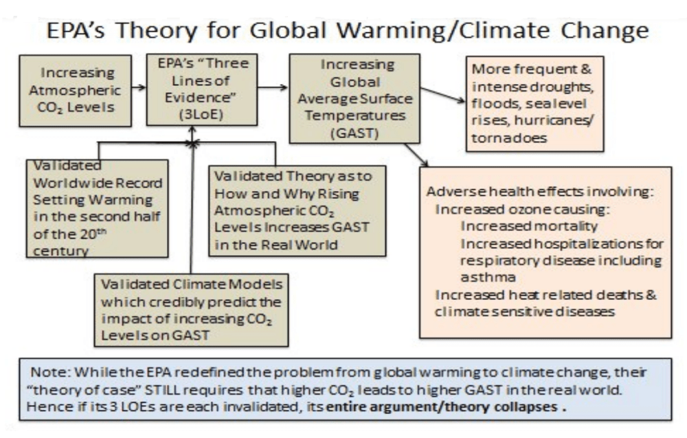
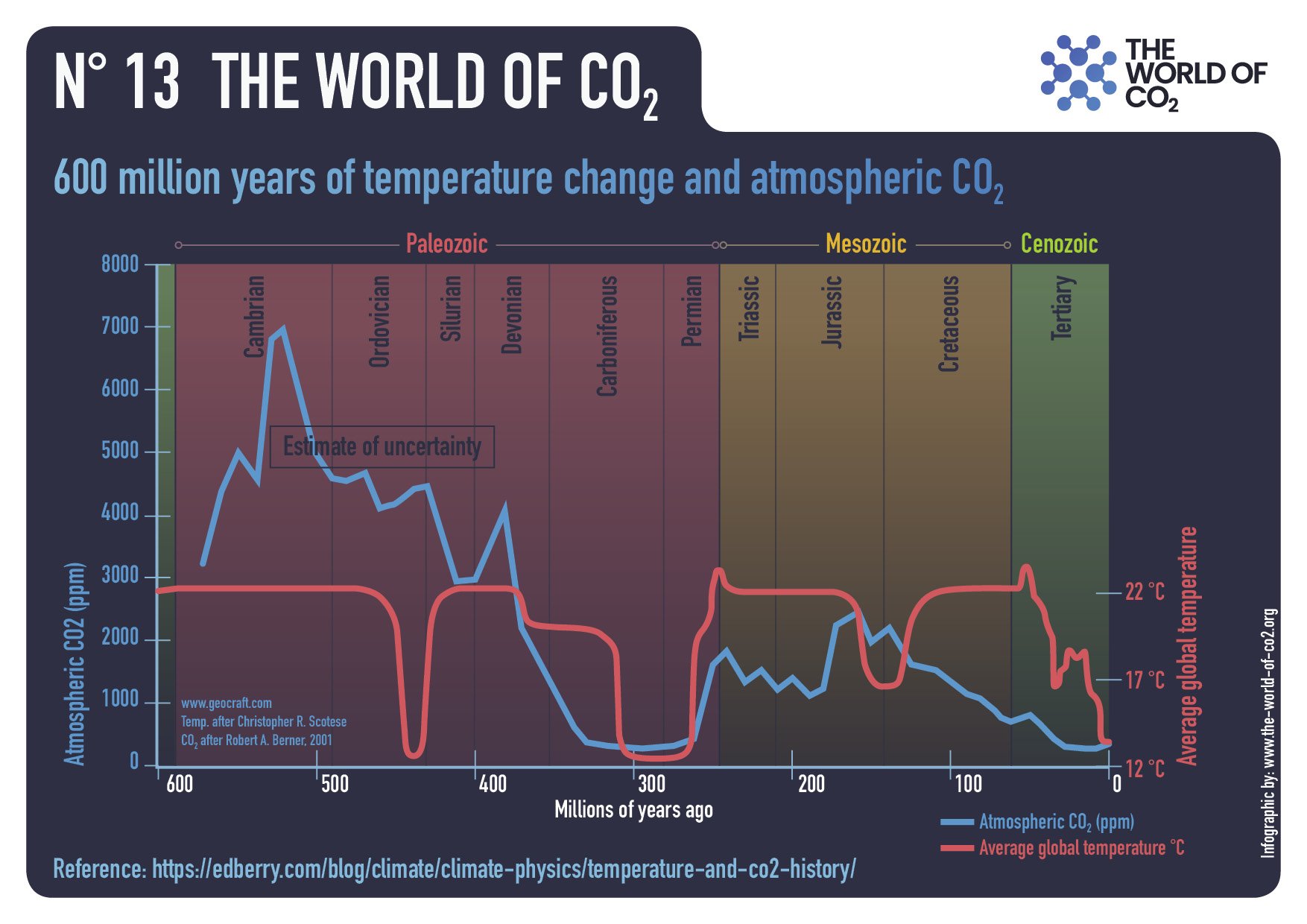
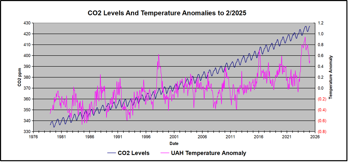
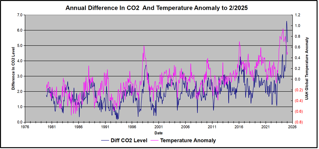
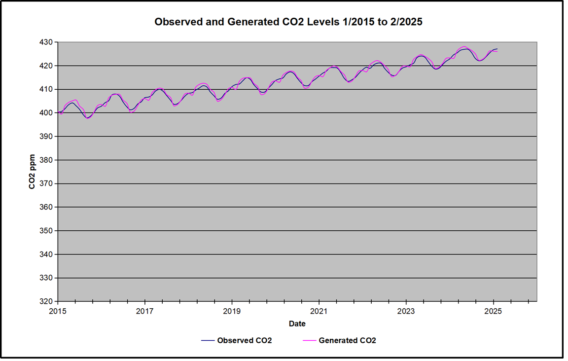
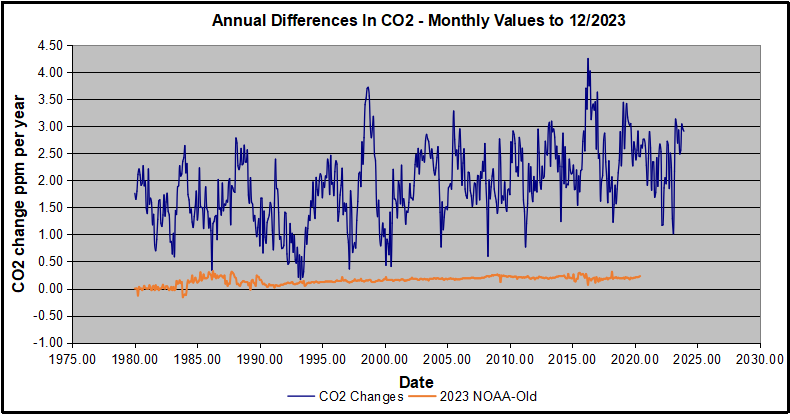
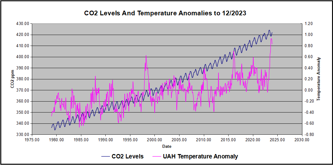
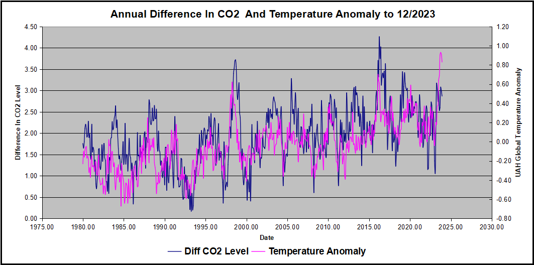
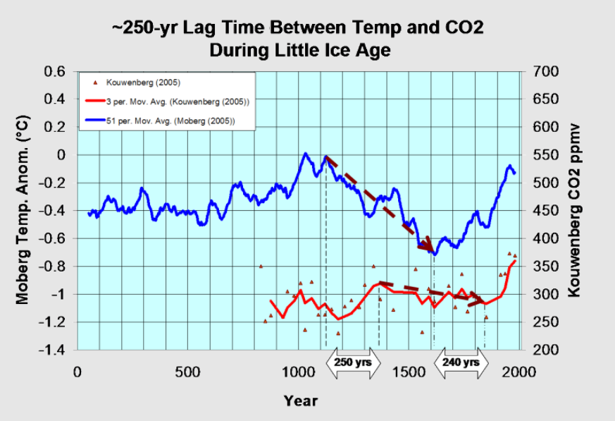
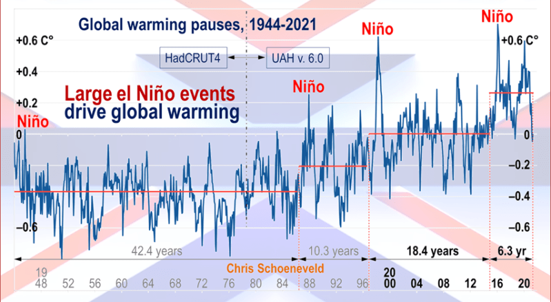
The 3 Lines of Evidence can all be challenged by scientific studies since the 2009 ruling.  The temperature records have been adjusted over time and the validity of the measurements are uncertain.  The issues with climate models give many reasons to regard them as unfit for policy making.  And the claim that rising CO2 caused rising Global Average Surface Temperature (GAST) is dubious, both on grounds that CO2 Infrared activity declines with higher levels, and that temperature changes precede CO2 changes on all time scales from last month’s observations to ice core proxies spanning millennia.

Thus all the arrows claiming causal relations are flawed.  The rise of atmospheric CO2 is mostly nature’s response to warming, rather than the other way around. And the earth warming since the Little Ice Age (LIA) is a welcome recovery from the coldest period in the last 10,000 years.  Claims of extreme weather  and rising sea levels ignore that such events are ordinary in earth history.  And the health warnings are contrived in attributing them to barely noticeable warming temperatures.

Background on the Legal Precedents

This post was triggered by noticing an event some years ago.  Serial valve turner Ken Ward was granted a new trial by the Washington State Court of Appeals, and he was allowed to present a “necessity defense.”  This astonishingly bad ruling is reported approvingly by Kelsey Skaggs at Pacific Standard Why the Necessity Defense is Critical to the Climate Struggle. Excerpt below with my bolds.

A climate activist who was convicted after turning off an oil pipeline won the right in April to argue in a new trial that his actions were justified. The Washington State Court of Appeals ruled that Ken Ward will be permitted to explain to a jury that, while he did illegally stop the flow of tar sands oil from Canada into the United States, his action was necessary to slow catastrophic climate change.

The Skaggs article goes on to cloak energy vandalism with the history of civil disobedience against actual mistreatment and harm.  Nowhere is it recognized that the brouhaha over climate change concerns future imaginary harm.  How could lawyers and judges get this so wrong?  It can only happen when an erroneous legal precedent can be cited to spread a poison in the public square.  So I went searching for the tree producing all of this poisonous fruit. The full text of the April 8, 2019, ruling is here.

A paper at Stanford Law School (where else?) provides a good history of the necessity defense as related to climate change activism The Climate Necessity Defense: Proof and Judicial Error in Climate Protest Cases Excerpts in italics with my bolds.

My perusal of the text led me to the section where the merits are presented.

The typical climate necessity argument is straightforward. The ongoing effects of climate change are not only imminent, they are currently occurring; civil disobedience has been proven to contribute to the mitigation of these harms, and our political and legal systems have proven uniquely ill-equipped to deal with the climate crisis, thus creating the necessity of breaking the law to address it. As opposed to many classic political necessity defendants, such as anti-nuclear power protesters, climate activists can point to the existing (rather than speculative) nature of the targeted harm and can make a more compelling case that their protest activity (for example, blocking fossil fuel extraction) actually prevents some quantum of harm produced by global warming. pg.78

What?  On what evidence is such confidence based?  Later on (page 80), comes this:

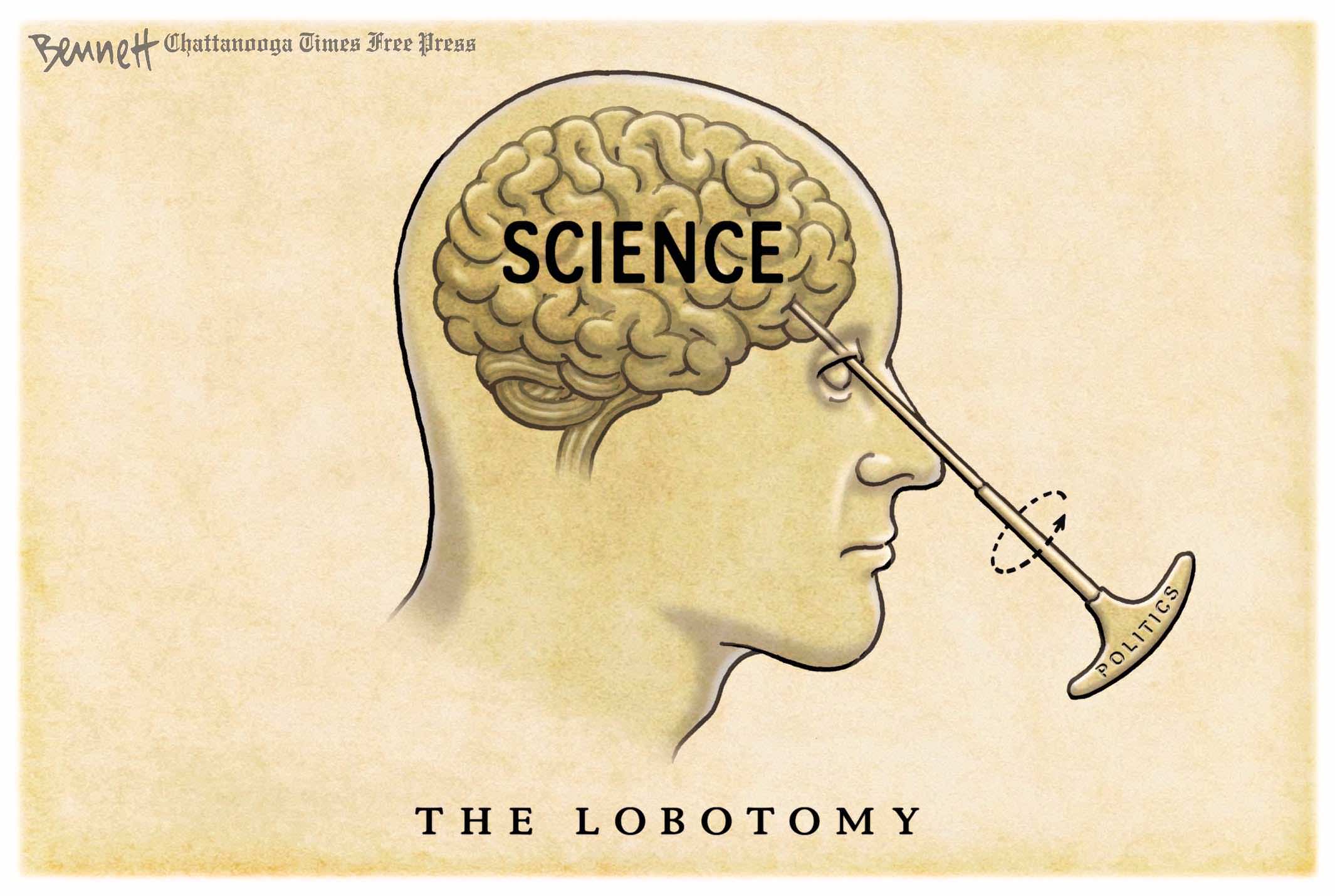
Second, courts’ focus on the politics of climate change distracts from the scientific issues involved in climate necessity cases. There may well be political disagreement over the realities and effects of climate change, but there is little scientific disagreement, as the Supreme Court has noted.131

131 Massachusetts v. E.P.A., 549 U.S. 497, 499 (2007) (“The harms associated with climate change are serious and well recognized . . . [T]he relevant science and a strong consensus among qualified experts indicate that global warming threatens, inter alia, a precipitate rise in sea levels by the end of the century, severe and irreversible changes to natural ecosystems, a significant reduction in water storage in winter snowpack in mountainous regions with direct and important economic consequences, and an increase in the spread of disease and the ferocity of weather events.”).

The roots of this poisonous tree are found in citing the famous Massachusetts v. E.P.A. (2007) case decided by a 5-4 opinion of Supreme Court justices (consensus rate: 56%).  But let’s see in what context lies that reference and whether it is a quotation from a source or an issue addressed by the court.  The majority opinion was written by Justice Stevens, with dissenting opinions from Chief Justice Roberts and Justice Scalia.  All these documents are available at sureme.justia.com Massachusetts v. EPA, 549 U.S. 497 (2007)

From the Majority Opinion:

A well-documented rise in global temperatures has coincided with a significant increase in the concentration of carbon dioxide in the atmosphere. Respected scientists believe the two trends are related. For when carbon dioxide is released into the atmosphere, it acts like the ceiling of a greenhouse, trapping solar energy and retarding the escape of reflected heat. It is therefore a species—the most important species—of a “greenhouse gas.” Source: National Research Council:

National Research Council 2001 report titled Climate Change: An Analysis of Some Key Questions (NRC Report), which, drawing heavily on the 1995 IPCC report, concluded that “[g]reenhouse gases are accumulating in Earth’s atmosphere as a result of human activities, causing surface air temperatures and subsurface ocean temperatures to rise. Temperatures are, in fact, rising.” NRC Report 1.

Calling global warming “the most pressing environmental challenge of our time,”[Footnote 1] a group of States,[Footnote 2] local governments,[Footnote 3] and private organizations,[Footnote 4] alleged in a petition for certiorari that the Environmental Protection Agency (EPA) has abdicated its responsibility under the Clean Air Act to regulate the emissions of four greenhouse gases, including carbon dioxide.  Specifically, petitioners asked us to answer two questions concerning the meaning of §202(a)(1) of the Act: whether EPA has the statutory authority to regulate greenhouse gas emissions from new motor vehicles; and if so, whether its stated reasons for refusing to do so are consistent with the statute.

EPA reasoned that climate change had its own “political history”: Congress designed the original Clean Air Act to address local air pollutants rather than a substance that “is fairly consistent in its concentration throughout the world’s atmosphere,” 68 Fed. Reg. 52927 (emphasis added); declined in 1990 to enact proposed amendments to force EPA to set carbon dioxide emission standards for motor vehicles, ibid. (citing H. R. 5966, 101st Cong., 2d Sess. (1990)); and addressed global climate change in other legislation, 68 Fed. Reg. 52927. Because of this political history, and because imposing emission limitations on greenhouse gases would have even greater economic and political repercussions than regulating tobacco, EPA was persuaded that it lacked the power to do so. Id., at 52928. In essence, EPA concluded that climate change was so important that unless Congress spoke with exacting specificity, it could not have meant the agency to address it.

Having reached that conclusion, EPA believed it followed that greenhouse gases cannot be “air pollutants” within the meaning of the Act. See ibid. (“It follows from this conclusion, that [greenhouse gases], as such, are not air pollutants under the [Clean Air Act’s] regulatory provisions …”).

Even assuming that it had authority over greenhouse gases, EPA explained in detail why it would refuse to exercise that authority. The agency began by recognizing that the concentration of greenhouse gases has dramatically increased as a result of human activities, and acknowledged the attendant increase in global surface air temperatures. Id., at 52930. EPA nevertheless gave controlling importance to the NRC Report’s statement that a causal link between the two “ ‘cannot be unequivocally established.’ ” Ibid. (quoting NRC Report 17). Given that residual uncertainty, EPA concluded that regulating greenhouse gas emissions would be unwise. 68 Fed. Reg. 52930.

The harms associated with climate change are serious and well recognized. Indeed, the NRC Report itself—which EPA regards as an “objective and independent assessment of the relevant science,” 68 Fed. Reg. 52930—identifies a number of environmental changes that have already inflicted significant harms, including “the global retreat of mountain glaciers, reduction in snow-cover extent, the earlier spring melting of rivers and lakes, [and] the accelerated rate of rise of sea levels during the 20th century relative to the past few thousand years … .” NRC Report 16.

In sum—at least according to petitioners’ uncontested affidavits—the rise in sea levels associated with global warming has already harmed and will continue to harm Massachusetts. The risk of catastrophic harm, though remote, is nevertheless real. That risk would be reduced to some extent if petitioners received the relief they seek. We therefore hold that petitioners have standing to challenge the EPA’s denial of their rulemaking petition.[Footnote 24]

In short, EPA has offered no reasoned explanation for its refusal to decide whether greenhouse gases cause or contribute to climate change. Its action was therefore “arbitrary, capricious, … or otherwise not in accordance with law.” 42 U. S. C. §7607(d)(9)(A). We need not and do not reach the question whether on remand EPA must make an endangerment finding, or whether policy concerns can inform EPA’s actions in the event that it makes such a finding. Cf. Chevron U. S. A. Inc. v. Natural Resources Defense Council, Inc., 467 U. S. 837, 843–844 (1984). We hold only that EPA must ground its reasons for action or inaction in the statute.

My Comment: Note that the citations of scientific proof were uncontested assertions by petitioners.  Note also that the majority did not rule that EPA must make an endangerment finding:  “We hold only that EPA must ground its reasons for action or inaction in the statute.”

From the Minority Dissenting Opinion

It is not at all clear how the Court’s “special solicitude” for Massachusetts plays out in the standing analysis, except as an implicit concession that petitioners cannot establish standing on traditional terms. But the status of Massachusetts as a State cannot compensate for petitioners’ failure to demonstrate injury in fact, causation, and redressability.

When the Court actually applies the three-part test, it focuses, as did the dissent below, see 415 F. 3d 50, 64 (CADC 2005) (opinion of Tatel, J.), on the State’s asserted loss of coastal land as the injury in fact. If petitioners rely on loss of land as the Article III injury, however, they must ground the rest of the standing analysis in that specific injury. That alleged injury must be “concrete and particularized,” Defenders of Wildlife, 504 U. S., at 560, and “distinct and palpable,” Allen, 468 U. S., at 751 (internal quotation marks omitted). Central to this concept of “particularized” injury is the requirement that a plaintiff be affected in a “personal and individual way,” Defenders of Wildlife, 504 U. S., at 560, n. 1, and seek relief that “directly and tangibly benefits him” in a manner distinct from its impact on “the public at large,” id., at 573–574. Without “particularized injury, there can be no confidence of ‘a real need to exercise the power of judicial review’ or that relief can be framed ‘no broader than required by the precise facts to which the court’s ruling would be applied.’ ” Warth v. Seldin, 422 U. S. 490, 508 (1975) (quoting Schlesinger v. Reservists Comm. to Stop the War, 418 U. S. 208, 221–222 (1974)).

The very concept of global warming seems inconsistent with this particularization requirement. Global warming is a phenomenon “harmful to humanity at large,” 415 F. 3d, at 60 (Sentelle, J., dissenting in part and concurring in judgment), and the redress petitioners seek is focused no more on them than on the public generally—it is literally to change the atmosphere around the world.

If petitioners’ particularized injury is loss of coastal land, it is also that injury that must be “actual or imminent, not conjectural or hypothetical,” Defenders of Wildlife, supra, at 560 (internal quotation marks omitted), “real and immediate,” Los Angeles v. Lyons, 461 U. S. 95, 102 (1983) (internal quotation marks omitted), and “certainly impending,” Whitmore v. Arkansas, 495 U. S. 149, 158 (1990) (internal quotation marks omitted).

As to “actual” injury, the Court observes that “global sea levels rose somewhere between 10 and 20 centimeters over the 20th century as a result of global warming” and that “[t]hese rising seas have already begun to swallow Massachusetts’ coastal land.” Ante, at 19. But none of petitioners’ declarations supports that connection. One declaration states that “a rise in sea level due to climate change is occurring on the coast of Massachusetts, in the metropolitan Boston area,” but there is no elaboration. Petitioners’ Standing Appendix in No. 03–1361, etc. (CADC), p. 196 (Stdg. App.). And the declarant goes on to identify a “significan[t]” non-global-warming cause of Boston’s rising sea level: land subsidence. Id., at 197; see also id., at 216. Thus, aside from a single conclusory statement, there is nothing in petitioners’ 43 standing declarations and accompanying exhibits to support an inference of actual loss of Massachusetts coastal land from 20th century global sea level increases. It is pure conjecture.

The Court ignores the complexities of global warming, and does so by now disregarding the “particularized” injury it relied on in step one, and using the dire nature of global warming itself as a bootstrap for finding causation and redressability.

Petitioners are never able to trace their alleged injuries back through this complex web to the fractional amount of global emissions that might have been limited with EPA standards. In light of the bit-part domestic new motor vehicle greenhouse gas emissions have played in what petitioners describe as a 150-year global phenomenon, and the myriad additional factors bearing on petitioners’ alleged injury—the loss of Massachusetts coastal land—the connection is far too speculative to establish causation.

From Justice Scalia’s Dissenting Opinion

Even on the Court’s own terms, however, the same conclusion follows. As mentioned above, the Court gives EPA the option of determining that the science is too uncertain to allow it to form a “judgment” as to whether greenhouse gases endanger public welfare. Attached to this option (on what basis is unclear) is an essay requirement: “If,” the Court says, “the scientific uncertainty is so profound that it precludes EPA from making a reasoned judgment as to whether greenhouse gases contribute to global warming, EPA must say so.” Ante, at 31. But EPA has said precisely that—and at great length, based on information contained in a 2001 report by the National Research Council (NRC) entitled Climate Change Science:

“As the NRC noted in its report, concentrations of [greenhouse gases (GHGs)] are increasing in the atmosphere as a result of human activities (pp. 9–12). It also noted that ‘[a] diverse array of evidence points to a warming of global surface air temperatures’ (p. 16). The report goes on to state, however, that ‘[b]ecause of the large and still uncertain level of natural variability inherent in the climate record and the uncertainties in the time histories of the various forcing agents (and particularly aerosols), a [causal] linkage between the buildup of greenhouse gases in the atmosphere and the observed climate changes during the 20th century cannot be unequivocally established. The fact that the magnitude of the observed warming is large in comparison to natural variability as simulated in climate models is suggestive of such a linkage, but it does not constitute proof of one because the model simulations could be deficient in natural variability on the decadal to century time scale’ (p. 17).

“The NRC also observed that ‘there is considerable uncertainty in current understanding of how the climate system varies naturally and reacts to emissions of [GHGs] and aerosols’ (p. 1). As a result of that uncertainty, the NRC cautioned that ‘current estimate of the magnitude of future warming should be regarded as tentative and subject to future adjustments (either upward or downward).’ Id. It further advised that ‘[r]educing the wide range of uncertainty inherent in current model predictions of global climate change will require major advances in understanding and modeling of both (1) the factors that determine atmospheric concentrations of [GHGs] and aerosols and (2) the so-called “feedbacks” that determine the sensitivity of the climate system to a prescribed increase in [GHGs].’ Id.

“The science of climate change is extraordinarily complex and still evolving. Although there have been substantial advances in climate change science, there continue to be important uncertainties in our understanding of the factors that may affect future climate change and how it should be addressed. As the NRC explained, predicting future climate change necessarily involves a complex web of economic and physical factors including: Our ability to predict future global anthropogenic emissions of GHGs and aerosols; the fate of these emissions once they enter the atmosphere (e.g., what percentage are absorbed by vegetation or are taken up by the oceans); the impact of those emissions that remain in the atmosphere on the radiative properties of the atmosphere; changes in critically important climate feedbacks (e.g., changes in cloud cover and ocean circulation); changes in temperature characteristics (e.g., average temperatures, shifts in daytime and evening temperatures); changes in other climatic parameters (e.g., shifts in precipitation, storms); and ultimately the impact of such changes on human health and welfare (e.g., increases or decreases in agricultural productivity, human health impacts). The NRC noted, in particular, that ‘[t]he understanding of the relationships between weather/climate and human health is in its infancy and therefore the health consequences of climate change are poorly understood’ (p. 20). Substantial scientific uncertainties limit our ability to assess each of these factors and to separate out those changes resulting from natural variability from those that are directly the result of increases in anthropogenic GHGs.

“Reducing the wide range of uncertainty inherent in current model predictions will require major advances in understanding and modeling of the factors that determine atmospheric concentrations of greenhouse gases and aerosols, and the processes that determine the sensitivity of the climate system.” 68 Fed. Reg. 52930.

I simply cannot conceive of what else the Court would like EPA to say.

Conclusion

Justice Scalia laid the axe to the roots of this poisonous tree.  Even the scientific source document relied on by the majority admits that claims of man made warming are conjecture without certain evidence.  This case does not prove CAGW despite it being repeatedly cited as though it did.

2025 The Legal Landscape Has Shifted For EPA

But much has changed in the legal landscape in recent years that will give opponents to Zeldin’s effort an uphill battle to fight. First is the changed make-up of the Supreme Court. When the Massachusetts v. EPA case was decided in 2007, the Court was evenly divided, consisting of four conservatives, four liberals, and Anthony Kennedy, a moderate who served as the Court’s “swing vote” in many major decisions. Kennedy was the deciding vote in that case, siding with the four liberal justices.

But conservatives hold an overwhelming 6-3 majority on today’s Supreme Court. While Chief Justice John Roberts and Associate Justice Amy Coney Barrett have occasionally sided with the Court’s three liberal justices in a handful of decisions, there is little reason to think that would happen in a reconsideration of the Massachusetts v. EPA case. That seems especially true for Justice Roberts, who wrote the dissenting opinion in the 2007 decision.

The Supreme Court’s 2024 decision in the Loper Bright Industries v. EPA case could present another major challenge for Zeldin’s opponents to overcome. In a 6-3 decision in that case, the Court reversed the longstanding Chevron Deference legal doctrine.

As I wrote at the time, [w]hen established in 1984 in a unanimous, 6-0 decision written by Justice John Paul Stevens, Chevron instructed federal courts to defer to the judgment of legal counsel for the regulatory agencies when such regulations were challenged via litigation. Since that time, agencies focused on extending their authority well outside the original intents of the governing statutes have relied on the doctrine to ensure they will not be overturned.

The existence of the Chevron deference has worked to ensure the judiciary branch of government has also been largely paralyzed to act decisively to review and overrule elements of the Biden agenda whenever the EPA, Bureau of Land Management or other agencies impose regulations that may lie outside the scope and intent of the governing statutes. In effect, this doctrine has served as a key enabler of the massive growth of what has come to be known as the US administrative state.

The question now becomes whether the current Supreme Court with its strong conservative majority will uphold its reasoning in Massachusetts v. EPA in the absence of the Chevron Deference.

The Bottom Line For Zeldin And EPA

Opponents of the expansion of EPA air regulations by the Obama and Biden presidencies have long contended that the underpinnings for those actions – Massachusetts v. EPA and the 2009 endangerment finding – were a classic legal house of cards that would ultimately come falling down when the politics and makeup of the Supreme Court shifted.

Trump and Zeldin are betting that both factors are now in favor of these major actions at EPA. Only time, and an array of major court battles to come, will tell.  [Source: David Blackmon at Forbes]

Footnote:  

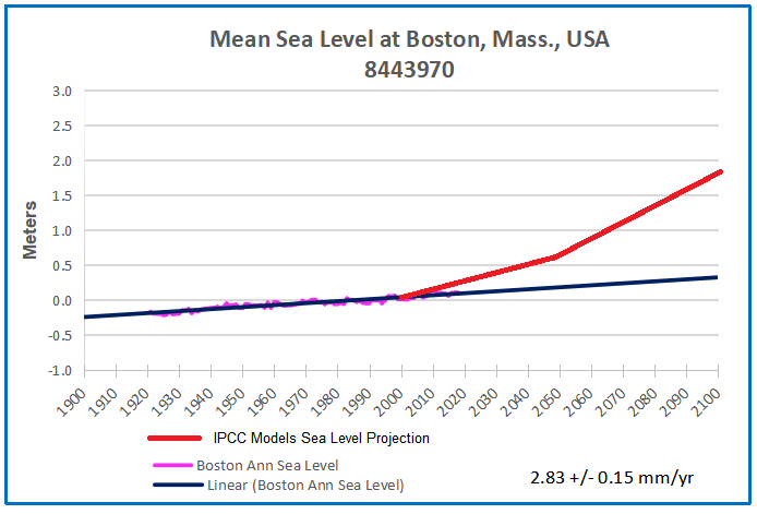
Taking the sea level rise projected by Sea Change Boston, and through the magic of CAI (Computer-Aided Imagining), we can compare to tidal gauge observations at Boston:


Don’t Fall for Carney’s Carbon Tax Trick

Kenneth Green explains in his Toronto Sun article Carney’s climate plan will keep costing Canadians money.  Excerpts in italics with my bolds and added images.

Mark Carney, our next prime minister, has floated a climate policy plan that he says will be better for Canadians than the “divisive (read: widely hated) consumer carbon tax.”

But in reality, Carney’s plan is an exercise in misdirection. Instead of paying the “consumer carbon tax” directly and receiving carbon rebates, Canadians will pay more via higher prices for products that flow from Canada’s “large industrial emitters,” who Carney plans to saddle with higher carbon taxes, indirectly imposing the consumer carbon tax by passing those costs onto Canadians.

Carney also wants to shift government subsidies to consumer products of so-called “clean technologies.”    As Carney told the National Observer, “We’re introducing changes so that if you decide to insulate your home, install a heat pump, or switch to a fuel-efficient car, those companies will pay you — not the taxpayer, not the government, but those companies.”

What Carney does not mention is that much of the costs imposed on “those companies” will also be folded into the costs of the products consumers buy, while the cause of rising prices will be less distinguishable and attributable to government action.

Moreover, Carney says he wants to make Canada a “clean energy superpower” and “expand and modernize our energy infrastructure so that we are less dependent on foreign suppliers, and the United States as a customer.” But this too is absurd. Far from being in any way poised to become a “clean energy superpower,” Canada likely won’t meet its own projected electricity demand by 2050 under existing environmental regulations.

For example, to generate the electricity needed through 2050 solely with solar power, Canada would need to build 840 solar-power generation stations the size of Alberta’s Travers Solar Project, which would take about 1,700 construction years to accomplish.

If we went with wind power to meet future demand, Canada would need to build 574 wind power installations the size of Quebec’s Seigneurie de Beaupre wind-power station, which would take about 1,150 construction years to accomplish. And if we relied solely on hydropower, we’d need to build 134 hydro-power facilities the size of the Site C power station in British Columbia, which would take 938 construction years to accomplish.

Finally, if we relied solely on nuclear power, we’d need to construct 16 new nuclear plants the size of Ontario’s Bruce Nuclear Generating Station, taking “only” 112 construction years to accomplish.

Again, Mark Carney’s climate plan is an exercise in misdirection — a rhetorical sleight of hand to convince Canadians that he’ll lighten the burden on taxpayers and shift away from the Trudeau government’s overzealous climate policies of the past decade. But scratch the surface of the Carney plan and you’ll see climate policies that will hit Canadian consumers harder, with likely higher prices for goods and services.

As a federal election looms, Canadians should demand from all candidates — no matter their political stripe — a detailed plan to rekindle Canada’s energy sector and truly lighten the load for Canadians and their families.

Minefield to Defuse EPA GHG Endangerment Finding

When first using this image, I was noting how naive were politicians (the Brits, for example) to legislate future CO2 emissions reductions, opening themselves up to lawsuits and legal constraints on policy decisions.  Now the same advice applies to the Trump administration targeting the root of the poisonous tree of climate alarmism.  First the lay of the land from EPA Director Zeldin, in italics with my bolds:

Trump EPA Kicks Off Formal Reconsideration of Endangerment Finding with Agency Partners

EPA Press Office (press@epa.gov)

WASHINGTON – U.S. Environmental Protection Agency (EPA) Administrator Lee Zeldin announced the agency will be kicking off a formal reconsideration of the 2009 Endangerment Finding in collaboration with the Office of Management and Budget (OMB) and other relevant agencies. EPA also intends to reconsider all of its prior regulations and actions that rely on the Endangerment Finding.

Administrator Zeldin: “After 16 years, EPA will formally reconsider the Endangerment Finding.”  “The Trump Administration will not sacrifice national prosperity, energy security, and the freedom of our people for an agenda that throttles our industries, our mobility, and our consumer choice while benefiting adversaries overseas. We will follow the science, the law, and common sense wherever it leads, and we will do so while advancing our commitment towards helping to deliver cleaner, healthier, and safer air, land, and water.”

White House OMB Director Russ Vought: “EPA’s regulation of the climate affects the entire national economy—jobs, wages, and family budgets. It’s long overdue to look at the impacts on our people of the underlying Obama endangerment finding.” 

Secretary of the Interior Doug Burgum: “The United States produces energy smarter, cleaner, and safer than anywhere else in the world. To achieve President Trump’s vision for energy dominance, we are prioritizing innovation over regulation to attain an affordable, reliable, clean, and secure energy future for all Americans.”

Energy Secretary Chris Wright:  “The 2009 Endangerment finding has had an enormously negative impact on the lives of the American people. For more than 15 years, the U.S. government used the finding to pursue an onslaught of costly regulations – raising prices and reducing reliability and choice on everything from vehicles to electricity and more. It’s past time the United States ensures the basis for issuing environmental regulations follows the science and betters human lives.”

Transportation Secretary Duffy:  “Thanks to President Trump’s leadership and the hard work of Administrator Zeldin, we are taking another important step toward ushering in a golden age of transportation. The American people voted for a government that prioritizes affordable, safe travel and lets them choose the vehicles they drive. Today we are delivering on that promise, and this will allow the DOT to accelerate its work on new vehicle fuel economy standards that will lower car prices and no longer force Americans to purchase electric vehicles they don’t want.” 

Office of Information and Regulatory Affairs Administrator Jeff Clark:  “Since 2009, I’ve consistently argued that the endangerment finding required a consideration of downstream costs imposed on both mobile sources like cars and stationary sources like factories. Under the enlightened leadership of President Trump and Administrator Zeldin, the time for fresh thought has finally arrived.”

In President Trump’s Day One Executive Order, “Unleashing American Energy,” he gave the EPA Administrator a 30-day deadline to submit recommendations on the legality and continuing applicability of the 2009 Endangerment Finding. After submitting these recommendations, EPA can now announce its intent to reconsider the 2009 Endangerment Finding.

When EPA made the Endangerment Finding in 2009, the agency did not consider any aspect of the regulations that would flow from it. EPA’s view then was that the Finding itself did not impose any costs, and that EPA could not consider future costs when making the Finding. EPA has subsequently relied on the Endangerment Finding as part of its justification for seven vehicle regulations with an aggregate cost of more than one trillion dollars, according to figures in EPA’s own regulatory impact analyses. The Endangerment Finding has also played a significant role in EPA’s justification of regulations of other sources beyond cars and trucks.  

Congress tasked EPA under Section 202 of the Clean Air Act with regulating new motor vehicles when the Administrator determines that emissions of an air pollutant endanger public health and welfare. But the Endangerment Finding went about this task in what appears to be a flawed and unorthodox way. Contrary to popular belief, the Endangerment Finding did not directly find that carbon dioxide emissions from U.S. cars endanger public welfare. Instead, the Finding looks at a combination of emissions of six different gases—and cars don’t even emit all six. It then creatively added multiple leaps, arguing that the combined six gases contribute some mysterious amount above zero to climate change and that climate change creates some mysterious amount of endangerment above zero to public health. These mental leaps were the only way the Obama-Biden Administration could come to its preferred conclusion, even if it did not stick to the letter of the Clean Air Act.  

The Endangerment Finding acknowledges and identifies significant uncertainties in the science and assumptions used to justify the decision. In the 16 years since EPA issued the Endangerment Finding, the world has seen major developments in innovative technologies, science, economics, and mitigation. EPA has never before asked for public comment on the implications these developments have had on the Endangerment Finding, but now it will as part of the reconsideration process it intends to undertake. Additionally, major Supreme Court decisions in the intervening years, including Loper Bright Enterprises v. Raimondo, West Virginia v. EPA, Michigan v. EPA, and Utility Air Regulatory Group v. EPA, have provided new guidance on how the agency should interpret statutes to discern Congressional intent and ensure that its regulations follow the law.  

As part of this reconsideration process, EPA will leverage the expertise of the White House Budget Office, including the Office of Information and Regulatory Affairs, White House Office of Science and Technology Policy, National Oceanic and Atmospheric Administration, and other relevant agencies.  

It is in the best interest of the American people for EPA to ensure that any finding and regulations are based on the strongest scientific and legal foundation. The reconsideration of the Endangerment Finding and EPA’s regulations that have relied on it furthers this interest. The agency cannot prejudge the outcome of this reconsideration or of any future rulemaking. EPA will follow the Administrative Procedure Act and Clean Air Act, as applicable, in a transparent way for the betterment of the American people and the fulfillment of the rule of law.

This was announced in conjunction with a number of historic actions to advance President Trump’s Day One executive orders and Power the Great American Comeback. Combined, these announcements represent the greatest and most consequential day of deregulation in the history of the United States. The overhaul of the Endangerment Finding along with other massive rules represents the death of the Green New Scam and drives a dagger straight into the heart of the climate change religion. While accomplishing EPA’s core mission of protecting the environment, the agency is committed to fulfilling President Trump’s promise to unleash American energy, lower costs for Americans, revitalize the American auto industry, restore the rule of law, and give power back to states to make their own decisions.

Objections from the usual suspects

“This decision ignores science and the law,” David Doniger, senior strategist and attorney for climate and energy at the Natural Resources Defense Council, said in a statement. “Abdicating EPA’s clear legal duty to curb climate-changing pollution only makes sense if you consider who would benefit: the oil, coal, and gas magnates who handed the president millions of dollars in campaign contributions.”

Vickie Patton, the Environmental Defense Fund’s general counsel, said any move to undo the finding “would be reckless, unlawful, and ignore EPA’s fundamental responsibility to protect Americans from destructive climate pollution. We will vigorously oppose it.”

“They don’t have a winning hand. Having the power to do this doesn’t tell you anything about whether or not what they’re doing makes sense on the merits,” said Joseph Goffman, who ran EPA’s air office during the Biden administration. “They’ve got nothing on the merits.”

Michael Mann, a climate scientist at the University of Pennsylvania dismissed the EPA’s action as “just the latest form of Republican climate denial. They can no longer deny climate change is happening, so instead they’re pretending it’s not a threat, despite the overwhelming scientific evidence that it is, perhaps, the greatest threat that we face today.”

The Pathways and the Risks

Shuting Pomerleau gives insight into activists worries and the possibilities:  Is EPA’s Endangerment Finding at Risk?

If EPA’s endangerment finding is rescinded, it may not have any material impact on the agency’s legal basis for issuing future climate regulations on GHG emissions, since the IRA amended the CAA to grant explicit authority to the agency. Nevertheless, repealing the endangerment finding would likely create chaos and uncertainty for U.S. climate policy.

First, rescinding the endangerment finding would make it much easier for the Trump Administration to repeal the existing EPA GHG emissions regulations because the original legal basis for this authority would no longer exist. Under the Obama and Biden Administrations, EPA has issued several sector-based GHG emissions regulations using the endangerment finding as a legal basis.

Second, repealing the endangerment finding would immediately subject EPA to legal challenges that could last years. Before the dispute could be adjudicated by the courts, there would be considerable confusion and uncertainty over compliance with the existing regulations. This would negatively impact the regulatory environment for businesses, as they need durable and consistent policies to make long-term investment decisions.

From the perspective of policymaking, rescinding EPA’s endangerment finding puts a big question mark on the outlook of U.S. climate policies. Currently, at the federal level, the United States uses a patchwork of policies to mitigate GHG emissions, such as handing out massive clean energy tax subsidies under the IRA and relying on command-and-control EPA regulations. The IRA energy tax provisions will likely be subject to at least partial repeal in an upcoming 2025 reconciliation bill. Even if a future administration seeks to regulate GHG emissions via EPA rulemaking, it would take a long time, and generally such regulations are costly, inflexible, and vulnerable to legal challenges.

What to Expect Next

EPA to Accept Nominations for Science Boards

EPA Press Office (press@epa.gov)

WASHINGTON – Today, U.S. Environmental Protection Agency (EPA) Administrator Lee Zeldin announced that a notice will be published in the Federal Register seeking nominations for the Science Advisory Board (SAB) and Clean Air Scientific Advisory Committee (CASAC). Nominations will be accepted for 30 days following publication of the Federal Register notice.

“Reconstituting the Science Advisory Board and Clean Air Scientific Advisory Committee are critical to ensuring that the agency receives scientific advice consistent with its legal obligations to advance our core mission of protecting human health and the environment,” said EPA Administrator Zeldin. “I look forward to receiving nominations to build an independent group of advisors to aid the agency’s rulemaking.” 

In January, EPA announced its decision to reset these federal advisory committees
to reverse the politicization of SAB and CASAC under the Biden-Harris Administration.


Ocean Warms, Land Cools UAH February 2025

The post below updates the UAH record of air temperatures over land and ocean. Each month and year exposes again the growing disconnect between the real world and the Zero Carbon zealots.  It is as though the anti-hydrocarbon band wagon hopes to drown out the data contradicting their justification for the Great Energy Transition.  Yes, there was warming from an El Nino buildup coincidental with North Atlantic warming, but no basis to blame it on CO2.

As an overview consider how recent rapid cooling  completely overcame the warming from the last 3 El Ninos (1998, 2010 and 2016).  The UAH record shows that the effects of the last one were gone as of April 2021, again in November 2021, and in February and June 2022  At year end 2022 and continuing into 2023 global temp anomaly matched or went lower than average since 1995, an ENSO neutral year. (UAH baseline is now 1991-2020). Now we have had an usual El Nino warming spike of uncertain cause, unrelated to steadily rising CO2 and now dropping steadily.

For reference I added an overlay of CO2 annual concentrations as measured at Mauna Loa.  While temperatures fluctuated up and down ending flat, CO2 went up steadily by ~60 ppm, a 15% increase.

Furthermore, going back to previous warmings prior to the satellite record shows that the entire rise of 0.8C since 1947 is due to oceanic, not human activity.

gmt-warming-events

The animation is an update of a previous analysis from Dr. Murry Salby.  These graphs use Hadcrut4 and include the 2016 El Nino warming event.  The exhibit shows since 1947 GMT warmed by 0.8 C, from 13.9 to 14.7, as estimated by Hadcrut4.  This resulted from three natural warming events involving ocean cycles. The most recent rise 2013-16 lifted temperatures by 0.2C.  Previously the 1997-98 El Nino produced a plateau increase of 0.4C.  Before that, a rise from 1977-81 added 0.2C to start the warming since 1947.

Importantly, the theory of human-caused global warming asserts that increasing CO2 in the atmosphere changes the baseline and causes systemic warming in our climate.  On the contrary, all of the warming since 1947 was episodic, coming from three brief events associated with oceanic cycles. And now in 2024 we have seen an amazing episode with a temperature spike driven by ocean air warming in all regions, along with rising NH land temperatures, now dropping below its peak.

Chris Schoeneveld has produced a similar graph to the animation above, with a temperature series combining HadCRUT4 and UAH6. H/T WUWT

image-8

mc_wh_gas_web20210423124932

See Also Worst Threat: Greenhouse Gas or Quiet Sun?

February 2025 Ocean Warms, Land Cools banner-blog

With apologies to Paul Revere, this post is on the lookout for cooler weather with an eye on both the Land and the Sea.  While you heard a lot about 2020-21 temperatures matching 2016 as the highest ever, that spin ignores how fast the cooling set in.  The UAH data analyzed below shows that warming from the last El Nino had fully dissipated with chilly temperatures in all regions. After a warming blip in 2022, land and ocean temps dropped again with 2023 starting below the mean since 1995.  Spring and Summer 2023 saw a series of warmings, continuing into 2024 peaking in April, then cooling off to the present.

UAH has updated their TLT (temperatures in lower troposphere) dataset for February 2025. Due to one satellite drifting more than can be corrected, the dataset has been recalibrated and retitled as version 6.1 Graphs here contain this updated 6.1 data.  Posts on their reading of ocean air temps this month are ahead of the update from HadSST4.  I posted recently on SSTs January 2025 Oceans Still Cool. These posts have a separate graph of land air temps because the comparisons and contrasts are interesting as we contemplate possible cooling in coming months and years.

Sometimes air temps over land diverge from ocean air changes. In July 2024 all oceans were unchanged except for Tropical warming, while all land regions rose slightly. In August we saw a warming leap in SH land, slight Land cooling elsewhere, a dip in Tropical Ocean temp and slightly elsewhere.  September showed a dramatic drop in SH land, overcome by a greater NH land increase. This month has contrasting warming in ocean air anomalies, especially in SH, somewhat offset by land air cooling especially in NH.

Note:  UAH has shifted their baseline from 1981-2010 to 1991-2020 beginning with January 2021.   v6.1 data was recalibrated also starting with 2021. In the charts below, the trends and fluctuations remain the same but the anomaly values changed with the baseline reference shift.

Presently sea surface temperatures (SST) are the best available indicator of heat content gained or lost from earth’s climate system.  Enthalpy is the thermodynamic term for total heat content in a system, and humidity differences in air parcels affect enthalpy.  Measuring water temperature directly avoids distorted impressions from air measurements.  In addition, ocean covers 71% of the planet surface and thus dominates surface temperature estimates.  Eventually we will likely have reliable means of recording water temperatures at depth.

Recently, Dr. Ole Humlum reported from his research that air temperatures lag 2-3 months behind changes in SST.  Thus cooling oceans portend cooling land air temperatures to follow.  He also observed that changes in CO2 atmospheric concentrations lag behind SST by 11-12 months.  This latter point is addressed in a previous post Who to Blame for Rising CO2?

After a change in priorities, updates are now exclusive to HadSST4.  For comparison we can also look at lower troposphere temperatures (TLT) from UAHv6.1 which are now posted for February 2025.  The temperature record is derived from microwave sounding units (MSU) on board satellites like the one pictured above. Recently there was a change in UAH processing of satellite drift corrections, including dropping one platform which can no longer be corrected. The graphs below are taken from the revised and current dataset.

The UAH dataset includes temperature results for air above the oceans, and thus should be most comparable to the SSTs. There is the additional feature that ocean air temps avoid Urban Heat Islands (UHI).  The graph below shows monthly anomalies for ocean air temps since January 2015.

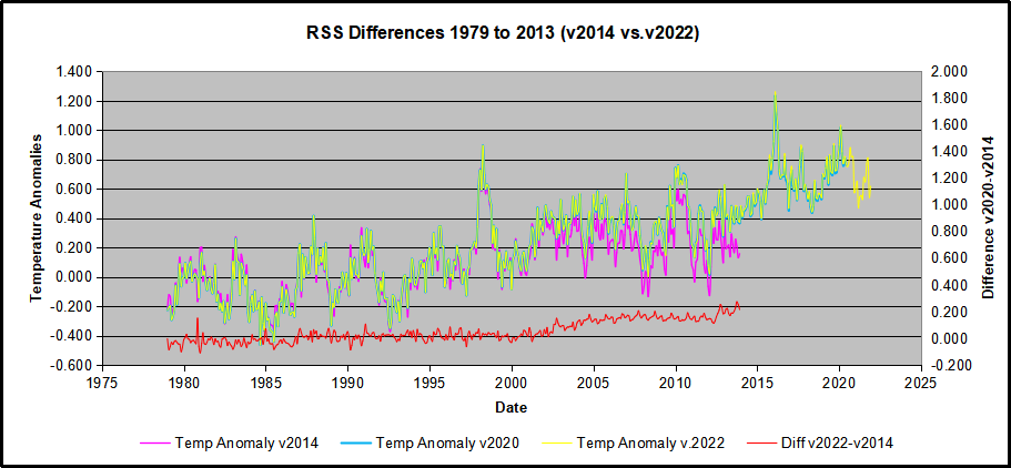
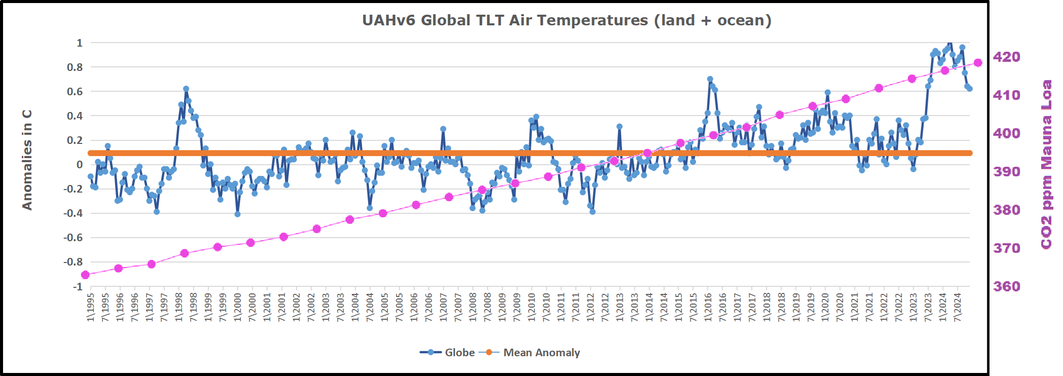
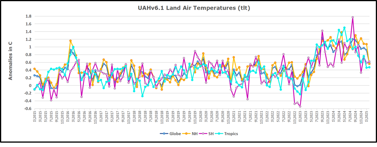
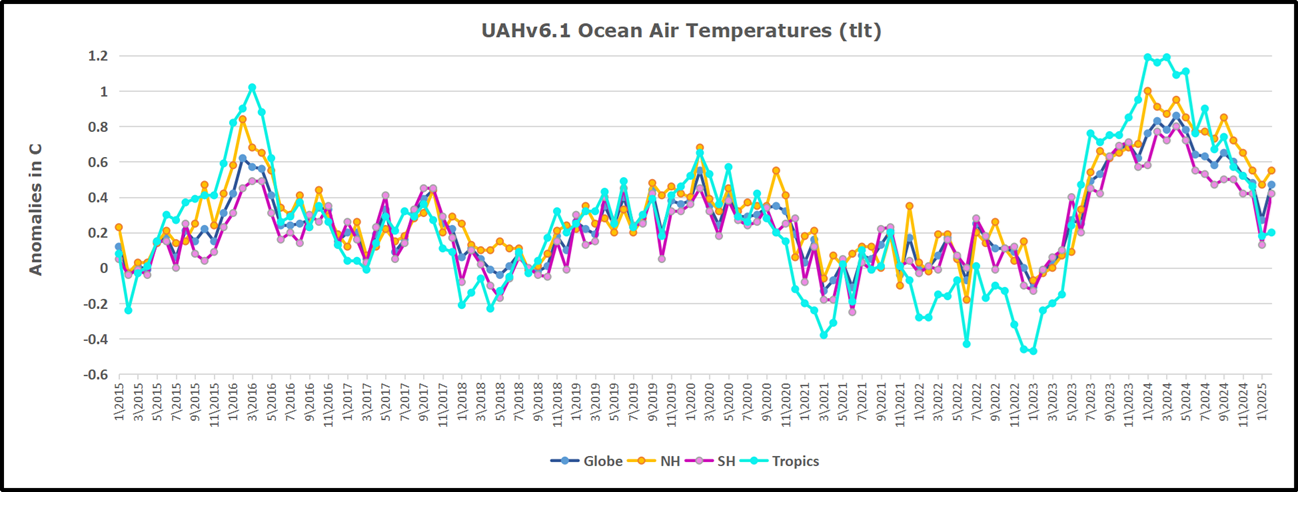
 In 2021-22, SH and NH showed spikes up and down while the Tropics cooled dramatically, with some ups and downs, but hitting a new low in January 2023. At that point all regions were more or less in negative territory.

After sharp cooling everywhere in January 2023, there was a remarkable spiking of Tropical ocean temps from -0.5C up to + 1.2C in January 2024.  The rise was matched by other regions in 2024, such that the Global anomaly peaked at 0.86C in April. Since then all regions have cooled down sharply.  In February 2025, SH rose from 0.1C to 0.4C pulling the Global ocean air anomaly up from 0.3C to 0.5C.

Land Air Temperatures Tracking in Seesaw Pattern

We sometimes overlook that in climate temperature records, while the oceans are measured directly with SSTs, land temps are measured only indirectly.  The land temperature records at surface stations sample air temps at 2 meters above ground.  UAH gives tlt anomalies for air over land separately from ocean air temps.  The graph updated for February is below.

Here we have fresh evidence of the greater volatility of the Land temperatures, along with extraordinary departures by SH land.  The seesaw pattern in Land temps is similar to ocean temps 2021-22, except that SH is the outlier, hitting bottom in January 2023. Then exceptionally SH goes from -0.6C up to 1.4C in September 2023 and 1.8C in  August 2024, with a large drop in between.  In November, SH and the Tropics pulled the Global Land anomaly further down despite a bump in NH land temps. February showed a sharp drop in NH land air temps from 1.07C down to 0.56C, pulling the Global land anomaly downward from 0.9C to 0.6C.

The Bigger Picture UAH Global Since 1980

The chart shows monthly Global Land and Ocean anomalies starting 01/1980 to present.  The average monthly anomaly is -0.03, for this period of more than four decades.  The graph shows the 1998 El Nino after which the mean resumed, and again after the smaller 2010 event. The 2016 El Nino matched 1998 peak and in addition NH after effects lasted longer, followed by the NH warming 2019-20.   An upward bump in 2021 was reversed with temps having returned close to the mean as of 2/2022.  March and April brought warmer Global temps, later reversed

With the sharp drops in Nov., Dec. and January 2023 temps, there was no increase over 1980. Then in 2023 the buildup to the October/November peak exceeded the sharp April peak of the El Nino 1998 event. It also surpassed the February peak in 2016. In 2024 March and April took the Global anomaly to a new peak of 0.94C.  The cool down started with May dropping to 0.9C, and in June a further decline to 0.8C.  October went down to 0.7C,  November and December dropped to 0.6C. February is down to 0.5C.

The graph reminds of another chart showing the abrupt ejection of humid air from Hunga Tonga eruption.

TLTs include mixing above the oceans and probably some influence from nearby more volatile land temps.  Clearly NH and Global land temps have been dropping in a seesaw pattern, nearly 1C lower than the 2016 peak.  Since the ocean has 1000 times the heat capacity as the atmosphere, that cooling is a significant driving force.  TLT measures started the recent cooling later than SSTs from HadSST4, but are now showing the same pattern. Despite the three El Ninos, their warming had not persisted prior to 2023, and without them it would probably have cooled since 1995.  Of course, the future has not yet been written.

Pushback Against EU World-wide ESG Rules

As Bloomberg reported, EU is attempting to force climate risk and ESG reporting on the whole world, not just its member nations.  

As trans-Atlantic relations grow increasingly fraught, Europe’s ESG regulations are becoming yet another flashpoint that threatens to sour ties.

The American Chamber of Commerce to the European Union (AmCham EU) says proposed revisions to the bloc’s environmental, social and governance rules don’t adequately protect US interests. The complaint is part of a growing US response to Europe’s ESG framework. Republican lawmakers call the rules “hostile” and warn that America’s jurisdictional sovereignty is at stake, while Commerce Secretary Howard Lutnick has said he’s willing to consider “trade tools” to retaliate.

The European Commission proposed changes last week that would rein in the scope of two major ESG laws: the Corporate Sustainability Reporting Directive and the Corporate Sustainability Due Diligence Directive. However, big international companies with business in the EU would still have to comply.

The upshot is that non-EU companies risk being ensnared by the bloc’s ESG rules, even for products that aren’t sold in the EU, said Kim Watts, senior policy manager for AmCham EU, whose members include Ford Motor Co., Exxon Mobil Corp. and Amazon.com Inc.

AmCham is worried that the EU “is going too far on extraterritoriality,” she said in an interview.

It’s a complaint that’s being backed up in even stronger terms by GOP members of Congress. In a letter sent shortly after the European Commission published its proposed revisions to the bloc’s ESG rules, the US lawmakers wrote to Treasury Secretary Scott Bessent and National Economic Council Director Kevin Hassett, warning of the “profound” implications of Europe’s due diligence directive for US businesses.

The lawmakers stated: “CSDDD imposes stringent due diligence requirements on in-scope companies, mandating the evaluation of supply chains to identify, mitigate, and eliminate human rights and environmental abuses as defined by United Nations (UN) and Organisation for Economic Cooperation and Development (OECD) principles.

“Furthermore, US firms will face increased litigation risks and potential enforcement actions from EU member states, with penalties under the Directive reaching up to 5% of a company’s global turnover.

“However, these principles have not been ratified by Congress, raising concerns about the legitimacy of EU enforcement against US companies based on these principles. Additionally, small businesses that supply larger companies will also be affected, even if their operations are solely within the US compliance efforts will require significant resource allocation, diverting funds away from critical areas such as research and development, talent acquisition, and investment.

R.I.P. Climate Back Radiation

Beware false and misleading Cartoons.

A brief recent video by Markus Ott explains why the notion of “back radiation” in Earth’s climate should be laid to rest.  I provide a transcript text in italics with my bolds and key exhibits.

Ott/Shula: The second law of thermodynamics and the greenhouse effect

This is the first of a short series of physics videos. This series is intended to be a follow up to Tom Shula’s presentation in which we can take more time to go into the fundamentals and derivations of our results.  Since Tom and I are attacking the foundations of modern climate science,  it makes sense to start with the thermodynamic aspects of the greenhouse effect.

In this video I will not talk about greenhouse gas molecules. I will look at the Green House Effect from the perspective of classical thermodynamics. Classical thermodynamics describes matter as a continuum and does not care about the atomic or molecular structure of matter.  The laws of thermodynamics have proven to be universally valid hypotheses, and theories that contradict the laws of thermodynamics have always proved to be wrong

In connection with the greenhouse effect, the second law of Thermodynamics is particularly interesting.  There are various equivalent formulations for the the second law of thermodynamics which states that thermal energy cannot be completely converted into other forms of energy.  Rudolf Clausius was the first to formulate the second law in the form that heat does not flow spontaneously from cold to hot bodies.  Later in 1865 he developed on that basis the concept of entropy.

Those who believe in thermodynamics categorize this statement as an eternal truth and therefore find it very difficult to understand how the greenhouse effect is supposed to work.  How can the atmosphere which is mostly colder than the Earth’s surface heat the Surface by means of back radiation, and by as much as 33°C?  Greenhouse effect believers like to refer to Carl Schwarzschild’s 1906 paper About the equilibrium of the solar atmosphere to answer this question.

In order to clarify this question of faith we will take a closer look at this much cited and probably rarely read article which was written in a German adequate to a highly educated man.  I posted a manual translation of the text on my substack page.  Without going into the details of his calculations we will look at how Schwarzschild comes to the conclusion that the sun’s atmosphere not only radiates outwards into space but that a significant proportion of radiation is also directed inwards towards the base of the sun’s atmosphere.

Such an inward or downward back radiation can also be measured at the bottom of the Earth’s atmosphere.  This observation is taken as a reason to postulate a similar radiation equilibrium in the Earth’s atmosphere.  The greenhouse effect is said to be the result of that back radiation.

The starting point for Schwarzschild’s article is the observation that the brightness of the visible solar disc is not evenly distributed.  The brightness decreases towards the edge.  The diagram shows the observed brightness distribution as a blue line. Schwarzschild compares two conceivable mechanisms of heat transport through the solar atmosphere in order to determine the cause of this brightness distribution. Heat transport through radiative transfer which requires a radiative equilibrium in the Solar atmosphere, and heat transport by convection with an adiabatic equilibrium in the Solar atmosphere.

He calculates how the brightness distribution on the solar disc should be for these two cases.  Because his results for the radiative equilibrium Orange Line in the diagram matched the observed brightness distribution Blue Line better than his results for the adiabatic equilibrium Gray Line,  he assumes that a radiative equilibrium prevails in the Solar atmosphere. We will disregard his description of the adiabatic equilibrium here, and restrict ourselves to his description of the radiative equilibrium.

Kirchhoff’s law of radiation plays a central role in Schwarzschild’s model. Kirchhoff’s law of radiation describes the relationship between absorption and emission of a real body in thermal equilibrium.  It states that radiation absorption and emission correspond to each other for a given wavelength. A body that absorbs well also radiates well.  This can be visualized as follows: We consider a body 2 that is located in a cavity of another body 1. Vacuum prevails in the intermediate space.   If both bodies have the same temperature the radiant power absorbed by Body 2 must be the same as the radiant power emitted by it because otherwise the temperature of body 2 would change.  This means that in thermal equilibrium Kirchhoff’s law of radiation represents a kind of radiation energy conservation law for body 2.

The layout of Schwarzschild’s radiative transfer model of the solar atmosphere is quite simple.  An unknown heat source in the core of the Sun generates heat;  a possible liquid outer core transports this heat by convection to the bottom of the solar atmosphere; the heat is then transported outwards into space solely by radiative transfer.  He does not go any further into the properties of the sun’s core.  He only assumes that the core heats the solar atmosphere evenly at its boundary surface.  It is very important that this heating occurs so evenly that convection currents do not form in the Solar atmosphere.

In Schwarzschild’s model the solar atmosphere is assumed to have the following properties:

♦  the solar atmosphere is stably stratified without convection;
♦  temperature and density increase continuously from the top of the atmosphere to the ground
♦  the vertical profile of temperature is smaller than the adiabatic vertical profile;
♦  each layer of the sun’s atmosphere absorbs and emits radiation without loss;
♦  the energy flow which flows from an unknown source inside the Sun through the solar atmosphere into the outer space is in a steady state.

Since a downwelling radiation is also measurable on the ground of Earth’s atmosphere, modern climate science assumes that Schwarzschild’s radiation transfer model is also applicable to our atmosphere.  Now let’s take a look at the applicability of  Schwarzschild’s  model to the Earth’s atmosphere.

It is striking that Schwarzschild has practically constructed his model around Kirchhoff’s law of radiation. He has to make a number of not particularly plausible assumptions in order to create a local thermal equilibrium between the layers of his solar atmosphere.  As mentioned before most of these assumptions serve to prevent convection in his model.  This is critically important because as soon as convection comes into play, the condition of local thermal equilibrium is no longer fulfilled.  The vertical convection currents and the associated turbulence destroy Schwarzschild’s homogeneous stratification of the atmosphere.  Large local temperature jumps occur Kirchhoff’s law of radiation is therefore no longer applicable.

To summarize and formulate this somewhat more abstractly:  In order to create the conditions for Pure radiation transport through the solar atmosphere Schwarzschild must construct an atmosphere with a very high degree of order.  In liquid or gaseous systems even minor disturbances will cause such a state to change into a disordered convective State.  Under convective conditions Kirchhoff’s law of radiation and thus the radiative transfer equation are not valid.

This transition to the convective state takes place with a large entropy gain.  It is therefore spontaneous and irreversible.  Accordingly, there should be no radiative transfer and no greenhouse effect in our troposphere since it is dominated by convection currents.

Look at a volume element under convective conditions such as those that prevail in our troposphere.  The volume element absorbs radiation and converts the radiation energy into heat. Before it can convert the heat back into radiation it is caught by a convection current and lifted.  This causes it to move into areas with lower ambient pressure.  It expands and performs volume work in the process.  It draws the energy for this volume work from its heat content and therefore cools down.  The amount of heat that the volume element has converted into volume work can no longer be converted back into radiation. The conservation of radiation energy is therefore no longer given.

Kirchhoff’s law of radiation can no longer be applied to the volume element. The entropy of the volume element increases, the process is irreversible lifting and acceleration.  Work performed by the volume element derives their energy from the heat content of the volume element and also contribute to the irreversibility of radiation absorption under convective conditions.  Global circulations also affect these processes but that will be discussed in another video.

I would like to point out that radiation absorption and emission are irreversible processes.  In themselves the reemission of radiation from an excited molecule occurs randomly in any direction.  This means that the information about the direction of the previously absorbed radiation is lost during emission The emitted Photon transfers part of its momentum to the emitting molecule. Its energy and therefore also its frequency are therefore different from that of the previously absorbed Photon.  Schwarzschild also excludes these effects through his choice of boundary conditions: steady state radiation flux and frequency independence of absorptivity and emission.

In one of my previous videos I made fun about the fact that the 33° greenhouse effect is calculated by assuming that the solar Radiance is homogeneously distributed over the Earth’s surface with 240 W per square meter. Now with a deeper understanding of Schwarzschild’s model we get an idea about the origin of this rather strange assumption.  In his radiation transfer model the base of the solar atmosphere is heated internally and homogenously by the solar core.  This homogeneous heating is very important since an inhomogeneous heating would cause convection which is incompatible with Kirchhoff’s law of radiation and would spoil his model.  In a rather hapless attempt to apply Schwarzschild’s radiation transfer model, the same is done to the externally and unevenly heated surface of the Earth.

To summarize briefly the irreversibility of radiation absorption in air under convective conditions makes back radiation and thus the greenhouse effect impossible.  This statement seems to be in direct contradiction to the observation that a downwelling atmospheric radiation can be measured at the bottom of the Earth’s atmosphere.  The diagram here shows the measured values from a measuring station near Munich.  In the next video I will show that back radiation is not what most people think of it to be, and how it is compatible with the laws of thermodynamics.

The most important takeaway from this video is that Kirchhoff’s law of radiation presents a kind of radiation energy conservation law, and that this radiation energy conservation is not given under convective conditions.  As far as I know all radiation transfer models assume a universal validity of Kirchhoff’s  law of radiation.  The only exception is at very high altitudes where the air molecules only very rarely collide with each other.  Since the results of the radiation transfer models are based on this false basic assumptions,  they are wrong.

That is not to say that Carl Schwarzschild’s work is nonsense.  His original idea is very applicable to transparent systems without convection; for example in the production of large telescope mirrors. The cooling behavior after the glass mass has solidified can be described very well using radiation transfer methods.

Footnote Regarding Observation of Downwelling IR near Earth Surface

Figure 1. This is a plot of the outgoing radiation spectrum from Earth. Within the normal IR thermometer and scanner range of 7.5 to 14 micrometers, only ozone (O3), which is mostly above cloud level absorbs and emits significant radiation. Within the 15 μm CO2 “divot” nearly all surface emissions are absorbed within 1.5 meters of the surface, at the edges of the divot, emissions are absorbed within 690 meters. There is very little absorption and emission by GHGs in the IR thermometer range in the troposphere, aka the atmospheric window.

From Andy May Beyond CO₂: Unraveling the Roles of Energy, Water Vapor, and Convection in Earth’s Atmosphere

Because the humid lower atmosphere is nearly opaque to most surface emitted radiation that is outside the atmospheric windows, surface emissions are absorbed by GHGs very close to the surface. According to Heinz Hug, at sea level, with a CO2 concentration of 357 PPM and 2.6% water vapor, 99.94% of all surface radiation in the main CO2 frequency band at about 15 μm is normally absorbed in the lower 10 meters of the atmosphere (Hug, 2012). Even at the edges of the deep CO2 frequency band (see figure 1, as well as figures 4 & 5 here) where any increase in the CO2 effect would be observed, 99.9% of the surface radiation is absorbed in the first 690 meters (Hug, 2000).

Heinz Hug goes on to say that is why climate change caused by CO2 cannot be measured directly in the laboratory and can only be modeled. In our opinion, the effect of CO2 is so small it will likely never be measured. In a similar fashion, any “back radiation” that makes it to the surface, outside atmospheric windows, is from the lower 10 meters of the atmosphere, the remaining emissions from the lower 10 meters of the atmosphere are captured by other greenhouse gases, almost always water vapor molecules.

Surface emissions in the frequencies that cannot be absorbed or emitted by GHGs, those in the so-called “atmospheric windows” are not captured, these are the frequencies utilized by IR thermometers and scanners, typically 7.5 to 14 micrometers as shown in figure 1. Water vapor is often a very weak absorber and emitter in portions of these windows. Carbon dioxide strongly absorbs and re-emits IR at two key frequencies: around 4.26 μm (microns) and 14.99 μm. The common vanadium oxide (VOx) based microbolometer long-wave infrared detectors cover wavelengths from 8-14 µm range. So, both CO2 absorption bands are outside the range of the common hand-held infrared thermometer/bolometer.

The radiation seen when IR thermometers and scanners are pointed at the sky is surface radiation scattered by atmospheric particles and clouds. The radiation seen by IR thermometers and scanners cannot be emitted by greenhouse gases or clouds because neither GHGs nor clouds emit in frequencies that can be detected by the devices. As noted in van Wijngaarden and Happer (2025) scattered longwave IR originates only in water droplets or ice or other particulates, there is negligible scattering of IR by molecules, especially in the atmospheric windows.

Background Paper with complete discussion

Missing Link in the GHE, Greenhouse Effect, by Thomas Shula – Markus Ott,  USA – Germany
2024.

Government Funding Corrupts Science, How to Stop It

William Briggs explains in his blog article The Case For Ending Government Funding of Science.  Excerpts in italics with my bolds and added images.

Direct government funding of science has to end.
Here is why, and what should replace it.

Some are making a big deal of a new paper in which “researchers found that between 1994-2023 not one of the 82 ‘climate science’ papers they identified had a financial or non-financial COI disclosure from at least one author.”

For the last decade, or moreI have been waving my arms around like a deranged monkey shouting that scientists, ante-Trump, did not view money from the government as tainted, biased, interested, dirty, suspicious or, especially, obliging. Instead, they thought of it as a natural and expected reward from the god Beneficence, i.e. Government, giving his people what they deserved, and they deserved because they were smart and spoke the right beliefs. They constantly told each other they were smart, anyway. And awarded credentials to each other to verify it.

Point is, when the moola was from Beneficence,
scientists saw NO conflict of interest.

They could not conceive of it existing. They thought their payoff was natural. And that was just as true when the money came from Beneficence’s brother god NGO. From the same source quoted above: “The research also found that:

“funding from NGOs was a significant predictor of studies reporting a positive association between climate change and hurricane behavior.”

No kidding.

How is it scientists claim purity, innocence, and disinterestedness when it is they themselves who hop on the Acela to DC and sit on the government committees that decide who gets the grant money from Beneficence? Of course the government has interest in the outcomes of research! How could they not? They asked for the research done specifically. They culled from consideration all proposals that were deemed hostile, inadequate, or politically incorrect. They, in cooperation with the gift getters, chose who lived and who died by the grant. Then Beneficence paid out! The government also asked for regular updates on the work which they asked and paid for.

I become exasperated every time I discuss this topic because I can’t see how this is not obvious. But it isn’t! We saw last week the (now) 3,400+ scientists who rage-signed a petition purportedly against Musk, but really to signal the scientists’ waning respect and fear over loss of all that free money they felt they so richly deserved.

Every source of money, save exceedingly rare completely
anonymous no-known-source gifts, has an interest.

When the sole source of funding, or near enough, is the government, the government thus has total interest and total control over the course of science. And those scientists who participate in the process, especially those who serve on grants committees, become part of the government, even though they hold no official position.

This system would be wonderful if the government was truly beneficent and wise. It is not. It is neither. I need only say to you DIE, “pregnant men”, “climate change”, “women in STEM”—and these are only a fraction of what has gone wrong—to prove that single-source behemoth control of science funding leads to absurdities.

And arrogance. Scientists in universities grew, as Eisenhower warned, too used to the largess, too hubristic over the “we pay; you do” system. That is not my phrase, but The Atlantic’s. They report on growing alarm over the new administration breathing Reality back into science (purging DIE), and from the loss of funds (like overhead). They say “The government has funded science and then largely left well enough alone.” This is as false as “pregnant men”. The government funded what it wanted! And it got what it wanted. They didn’t just leave pools of money from which scientists came and freely grazed. They controlled who got every cent.

Scientists are right to be frightened.
The new small cuts should only be the start.

 The entire grants apparatus, except perhaps for rare special exceptions (which I am not here prepared to name), ought to be dismantled. There are too many scientists, fed by too much money, which leads to too much bad science, which drags the entire system down. I have written about this scores of times and won’t justify that opinion more here.

Notice I do not say “do not fund science”. I say the government grants system ought to be abolished. Here are some ideas what could replace it.

If every source of money is interested, then spread the interest around so it’s not concentrated to serve one cracked master. This reduces the chance science becomes degraded and cancerous and calcified as it now is.

I’ve already written a good deal of science can be shunted to private interests, who are free to pursue that which interests them. That is the most obvious route. Pharmaceuticals rely on this, and they ain’t hurtin’ (Trump will soon sign an executive order banning p-values). Stop counting on universities to churn ideas which private interests might use. Instead, do it yourself, homegrown. A larger spend up front, but an even larger return on investment at the end.

Patronage is a traditional route. The best off should indulge in noblesse oblige. Which, of course, many do. But they give the money to universities, which are corrupted to the bone, not least because of all the government money, but also because of misguided Equality (too many kids go to university), and managerialism (universities have more administrators than professors). If, and once, universities are restored to their former glory, the rich can return and have buildings named after them.

For now, fund individual scientists,
who can be anywhere and not just campus bound.

Or not just for now, but forever. This is the idea of Jacob Shell. He would give university scientists large salaries, and no grants. See if you’re not crying “Amen!” at the end of this:

Academic freedom of inquiry is the opposite of the grant system. The two cannot cohabitate the same cosmos. Because academic grants exist, nobody in the academy is really intellectually free. If academics were really intellectually free, then there could not be such a thing as an academic grant.

Scientists would use their own money, however obtained, to fund their own research. Which would be whatever they wanted it to be. Or not. Groups of scientists could form bands and pool their money to do more expensive research. If they wanted. Or not.

This brilliant idea results immediately in far fewer scientists, which brings freedom. It instantly reduces publish or perish, since scientists won’t have to grub for grants. The breathing room bought by this is wonderful to imagine. If this is done at universities, the extra money to pay scientists would have to come from firing administrators and asssistants to the asssistant Deans. A giddy thought.

It’s not that scientists won’t have to beg for money from someone. It’s that they will have to beg from someones. It spreads the interest around. The system becomes more adversarial and independent and thus creative. It would indeed result in a reduction of science. That is a blessing.

It forces the government, which would be out of the business of funding scientists, to find scientists which support whatever programs the government loves, and convince those who have money to fund these scientists. That requires real work, and will be forever a path to corruption. But a tangled one, which slows the rot. Now, government pays scientists directly to give them the support for The Science, so politicians and announce “Follow The Science!” and pretend there is no taint.

Science needs to feel the pain of hugeous cuts. Pain is necessary to grow.
If anybody reading this has access to our new rulers,
get them not just to cut overhead, but cut it all.

See Also

Why Federalized Science is Rotten

SEC Climate Risk Rule is Entrapment

Stone Washington and William Happer explain the nefarious and ill-advised decree in their article SEC’s Climate Risk Disclosure Rule Would Compel Companies to Make Scientifically False and Misleading Disclosures.  Excerpts in italics with my bolds and added images.

In March last year, the Securities and Exchange Commission issued its climate risk disclosure rule, called “The Enhancement and Standardization of Climate-Related Disclosures for Investors.” 

It requires companies to report enormously costly and voluminous data on their carbon dioxide and other greenhouse gas (GHG) emissions. With this rule, the SEC seeks “to achieve the primary benefits of GHG emissions disclosure” for investors, including disclosure of “risks associated” with regulations such as President Biden’s “commitments to reduce economy-wide net greenhouse gas emissions … to reach net zero emissions by 2050.”

It will flood investors with pages upon pages of information. As to costs, the SEC’s own numbers found that the proposed rule would increase annual compliance costs from $3.8 billion to $10.2 billion, a $6.4 billion rise — more than all the accumulated SEC disclosure rules’ costs from SEC’s initiation in the 1930s to date – combined. Even though the final rule’s cost is less, the numbers indicate the order of magnitude. It may signal what the ultimate cost of future environmental disclosures would be, in addition to the ensuing fossil fuel divestment

The SEC assumes, like many, the Intergovernmental Panel on Climate Change claim the “evidence is clear that carbon dioxide (CO2) is the main driver of climate change,” including, the SEC asserts, “higher temperatures, sea level rise, and drought”, as well as “hurricanes, floods, tornadoes, and wildfires.”

However, the little-known accurate science is totally contrary to the SEC’s and IPCC’s premise. Co-author William Happer, an emeritus physics professor at Princeton, explains below how carbon dioxide and other GHGs do not cause any increased climate related risks. The SEC’s and IPCC’s claim is scientifically false. 

Thus, the SEC rule would compel companies to disclose scientifically false and misleading information about carbon dioxide and other GHG’s role in climate-related risks to investors. Accordingly, the SEC rule must be rescinded by the Trump Administration or ruled invalid by the courts, whichever is sooner.

Co-author Happer explains the accurate science in detail in a 28 page comment on the proposed SEC rule with Richard Lindzen, an emeritus physics professor at MIT. The comment explains why there are no added climate related risks caused by carbon dioxide. (The other greenhouse gases such as methane and nitrous oxide are too small to have any significant effect on the environment).

The SEC totally ignored and did not respond to the comment. Three of the many scientific reasons elaborated in the comment are:

First, Carbon Dioxide Now and at Higher Levels is a Weak Greenhouse Gas, So Reducing It to Net Zero Will Have a Negligible Effect on Temperatures

As a GHG, carbon dioxide’s ability to raise Earth’s temperature decreases rapidly as the atmospheric concentration increase.   The science is complex, but the scientific conclusion is simple. At today’s level of about 400 parts per million (ppm) and higher, large increases of carbon dioxide will cause negligible warming of the Earth.

The well-established theory of atmospheric heat transfer allows computing what happens when carbon dioxide’s concentration in the atmosphere increases, for example, doubling from today’s approximately 400 ppm to 800 ppm.   As to temperature, the result would be only a minuscule effect on temperature because carbon dioxide is now, and at higher levels, a weak greenhouse gas. Lindzen and Happer state:

“From now on … we could emit as much CO2 as we like, with little warming effect.” This also means that “our emissions from burning fossil fuels could have little impact on global warming. There is no climate emergency. No threat at all.” 

As to food, carbon dioxide creates more food when its level in the atmosphere increases. Doubling carbon dioxide from 400 ppm to 800 ppm would increase the amount of food available to people worldwide by roughly 40%, with a negligible effect on temperature.

Further, never mentioned, is that reducing carbon dioxide to Net Zero will reduce the amount of food available worldwide.

Second. The EPA’s MAGICC Model Confirms Carbon Dioxide Now and at Higher Levels is a Weak Greenhouse Gas, So Reducing It to Net Zero Will Have a Negligible Effect on Temperatures

The Environmental Protection Agency often uses a model for predicting temperature effects called the Model for Assessment of Greenhouse Gas-Induced Climate Change (MAGICC).  Our comment explains the MAGICC model confirms our conclusion:

“Reducing the current 40 Gigaton CO2 annual emissions worldwide and the 6 Gigaton annual U.S. CO2 emissions to ‘net zero’ would cause only tiny changes of … Earth’s surface temperature.”

Third. 600 Million Years of Carbon Dioxide Data Also Confirms Carbon Dioxide Now and at Higher Levels is a Weak Greenhouse Gas, So Reducing It to Net Zero Will Have a Negligible Effect on Temperatures

Our comment presents 600 million years of data on temperature and carbon dioxide levels that shows an inverse relationship most of the time. “For hundreds of millions of years, temperatures were low when CO2 levels were high, and temperatures were high when CO2 levels were low.”

“When CO2 was record high of about 7,000 ppm, temperatures were at a record low.”

Thus 600 million years of data also confirms carbon dioxide is now a weak greenhouse gas that cannot and does not drive climate change.

Finally, our comment details why the rule if adopted would help cause disastrous consequences for the poor, people worldwide, and future generations of Americans because it would reduce the amount of carbon dioxide in the atmosphere and the use of fossil fuels.

Therefore, science contradicts the SEC and IPCC’s premise that carbon dioxide and other greenhouse gases introduce climate-related risks. Such assumptions are scientifically false. Thus requiring companies to report their GHG data to investors interested in climate change would require them to report false and misleading information.

Accordingly, the new SEC leadership should immediately rescind its climate-related risks disclosure rule, or the courts should rule it invalid, whichever is sooner.

Finally, there are, of course, nature caused climate-related risks. For nature, the SEC explained, “it has required disclosure of certain environmental matters for the past 50 years,” including “disclosure of climate-related risks and their impacts on a registrant’s business or financial condition.”

Thus, the SEC has already taken care of them. Nothing else need be done.