Heat Wave Good Vibrations
Enjoy this wonderful hot summertime while it lasts. Don’t let the climate grinches get you down with their doomsday pronouncements. Chill out with Sunshine Reggae and let the good vibes get a lot stronger.
Enjoy this wonderful hot summertime while it lasts. Don’t let the climate grinches get you down with their doomsday pronouncements. Chill out with Sunshine Reggae and let the good vibes get a lot stronger.
Earlier in July, I pointed out Arctic ice extent displaying an “hockey stick” shape due to a surplus of ice compared to the 11 year average decline during this month. Now we are seeing more typical ice loss approaching the Mid-September annual minimum. The image above shows how Kara Sea lost more than 300k km2 of ice in the last two weeks, from 428k down to below 100k. That is less ice in Kara than last year, but matching 2015 and 2016 on this day. On the left you can also see Laptev Sea adding ~200k km2 of open water.
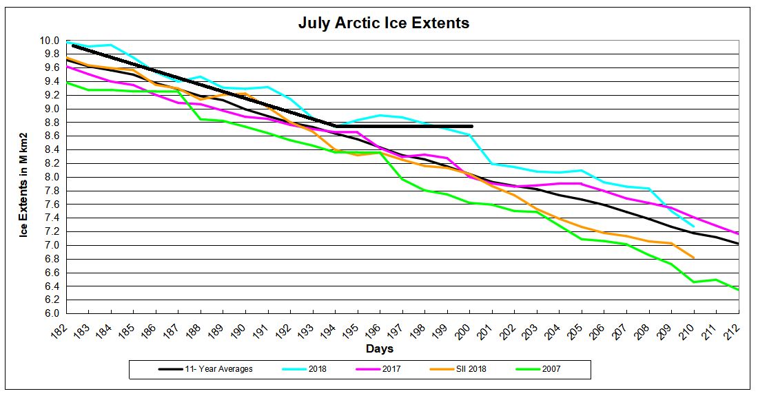
The graph above shows the mid-month “hockey stick” followed by ice extent declining more rapidly, now slightly below last year and slightly above the 11 year average. The gap over 2007 is still over 800k km2, and MASIE is showing about 500k km2 more than SII (NOAA Sea Ice Extent). At end of month, there will be a more complete report.

Iowa trivia: Refrain from Iowa Corn Song: “We’re from I-o-way, I-o-way, That’s where the tall corn grows.” Athletic teams that represent Iowa State University are called the “Cyclones,” after the devastating 1895 storms, the most extreme weather in state history. My mother was born and raised near Cedar Rapids, IA.
Today a website in Iowa reblogged my post Who to Blame for Rising CO2? Returning the favor I draw your attention to a concise, comprehensive and reasonable statement of their climate perspective. The website is Iowa Climate Science Education (Red title is link). Excerpts below from their position statement in italics with my bolds.
Scientists disagree about the causes and consequences of climate for several reasons. Climate is an interdisciplinary subject requiring insights from many fields. Very few scholars have mastery of more than one or two of these disciplines. Fundamental uncertainties arise from insufficient observational evidence and disagreements over how to interpret data and how to set the parameters of models. The Intergovernmental Panel on Climate Change (IPCC), created to find and disseminate research finding a human impact on global climate, is not a credible source. It is agenda-driven, a political rather than scientific body, and some allege it is corrupt. Finally, climate scientists, like all humans, can be biased. Origins of bias include careerism, grant-seeking, political views, and confirmation bias.
Probably the only “consensus” among climate scientists is that human activities can have an effect on local climate and that the sum of such local effects could hypothetically rise to the level of an observable global signal. The key questions to be answered, however, are whether the human global signal is large enough to be measured and if it is, does it represent, or is it likely to become, a dangerous change outside the range of natural variability? On these questions, an energetic scientific debate is taking place on the pages of peer-reviewed science journals.
In contradiction of the scientific method, IPCC assumes its implicit hypothesis – that dangerous global warming is resulting, or will result, from human-related greenhouse gas emissions – is correct and that its only duty is to collect evidence and make plausible arguments in the hypothesis’s favor. It simply ignores the alternative and null hypothesis, amply supported by empirical research, that currently observed changes in global climate indices and the physical environment are the result of natural variability.
The results of the global climate models (GCMs) relied on by IPCC are only as reliable as the data and theories “fed” into them. Most climate scientists agree those data are seriously deficient and IPCC’s estimate for climate sensitivity to CO2 is too high. We estimate a doubling of CO2 from pre-industrial levels (from 280 to 560 ppm) would likely produce a temperature forcing of 3.7 Wm-2 in the lower atmosphere, for about ~1°C of prima facie warming. The recently quiet Sun and extrapolation of solar cycle patterns into the future suggest a planetary cooling may occur over the next few decades.

In a similar fashion, all five of IPCC’s postulates, or assumptions, are readily refuted by real-world observations, and all five of IPCC’s claims relying on circumstantial evidence are refutable. For example, in contrast to IPCC’s alarmism, we find neither the rate nor the magnitude of the reported late twentieth century surface warming (1979–2000) lay outside normal natural variability, nor was it in any way unusual compared to earlier episodes in Earth’s climatic history. In any case, such evidence cannot be invoked to “prove” a hypothesis, but only to disprove one. IPCC has failed to refute the null hypothesis that currently observed changes in global climate indices and the physical environment are the result of natural variability.
Rather than rely exclusively on IPCC for scientific advice, policymakers should seek out advice from independent, nongovernment organizations and scientists who are free of financial and political conflicts of interest. Our conclusion, drawn from its extensive review of the scientific evidence, is that any human global climate impact is within the background variability of the natural climate system and is not dangerous. In the face of such facts, the most prudent climate policy is to prepare for and adapt to extreme climate events and changes regardless of their origin. Adaptive planning for future hazardous climate events and change should be tailored to provide responses to the known rates, magnitudes, and risks of natural change. Once in place, these same plans will provide an adequate response to any human-caused change that may or may not
emerge.
Policymakers should resist pressure from lobby groups to silence scientists who question the authority of IPCC to claim to speak for “climate science.” The distinguished British biologist Conrad Waddington wrote in 1941,
“It is important that scientists must be ready for their pet theories to turn out to be wrong. Science as a whole certainly cannot allow its judgment about facts to be distorted by ideas of what ought to be true, or what one may hope to be true.” (Waddington, 1941).
This prescient statement merits careful examination by those who continue to assert the fashionable belief, in the face of strong empirical evidence to the contrary, that human CO2 emissions are going to cause dangerous global warming.
Reference
Waddington, C.H. 1941. The Scientific Attitude. London, UK: Penguin Books.

/cdn.vox-cdn.com/uploads/chorus_image/image/56293121/total_solar_eclipse.0.jpg)
The last solar eclipse was in 2017. The totality in the picture lasted a little more than 2 minutes, while the process lasted about 2.5 hours.
One of the great disputes in climate research is between those (IPCC) who dismiss solar cycles as a factor in climate change and those who see correlations in the past and keep seeking to understand the mechanisms. To be clear, there is considerable agreement that earth’s atmosphere can and does reduce or increase the amount of incoming solar energy (albedo effect), thereby contributing to surface warming or cooling. The science and research into the “global dimming and brightening” is discussed in the post Nature’s Sunscreen.
The above image of the eclipse is intended to remind us that humans down through history have been terrified of the sun going dark because they knew intuitively that no sun means no life. A more modern and sophisticated concern is that even slightly falling energy from the sun brings cooling, ice and death. Quite apart from the sunscreen, this post is focused a different matter, namely that changes in the sun’s output radiation cause changes in earth climate parameters. One theory of such a mechanism is espoused by Henrik Svensmark and concerns solar particles effect upon albedo. That line of research is discussed in the post The Cosmoclimatology theory

A different investigation has been advanced by Dr.Indrani Roy, her most recent publication this month being a book Climate Variability and Sunspot Activity Analysis of the Solar Influence on Climate (H/T NoTricksZone).
The book is behind a paywall, but the abstract and chapter headings indicate a comprehensive approach.
Overview Climate Variability and Sunspot Activity (2018)
This book promotes a better understanding of the role of the sun on natural climate variability. It is a comprehensive reference book that appeals to an academic audience at the graduate, post-graduate and PhD level and can be used for lectures in climatology, environmental studies and geography.
This work is the collection of lecture notes as well as synthesized analyses of published papers on the described subjects. It comprises 18 chapters and is divided into three parts: Part I discusses general circulation, climate variability, stratosphere-troposphere coupling and various teleconnections. Part II mainly explores the area of different solar influences on climate. It also discusses various oceanic features and describes ocean-atmosphere coupling. But, without prior knowledge of other important influences on the earth’s climate, the understanding of the actual role of the sun remains incomplete. Hence, Part III covers burning issues such as greenhouse gas warming, volcanic influences, ozone depletion in the stratosphere, Arctic and Antarctic sea ice, etc. At the end of the book, there are few questions and exercises for students. This book is based on the lecture series that was delivered at the University of Oulu, Finland as part of M.Sc./ PhD module.
Chapter Titles
To better appreciate Roy’s viewpoint, two of her previous publications provide the evidence and analytical thought behind her conclusions. Published in 2010 with J.D. Haigh was Solar cycle signals in sea level pressure and sea surface temperature Excerpts in italics with my bolds.
Summary of SLP and SST signals
We identify solar cycle signals in the North Pacific in 155 years of sea level pressure and sea surface temperature data. In SLP we find in the North Pacific a weakening of the Aleutian Low and a northward shift of the Hawaiian High in response to higher solar activity, confirming the results of previous authors using different techniques. We also find a broad reduction in pressure across the equatorial region but not the negative anomaly in the sub-tropics detected by vL07. In SST we identify the warmer and cooler regions in the North Pacific found by vL07 but instead of the strong Cold Event-like signal in tropical SSTs we detect a weak WE-like pattern in the 155 year dataset.
We find that the peak SSN years of the solar cycles have often coincided with the negative phase of ENSO so that analyses, such as that of vL07, based on composites of peak SSN years find a La Nina response. As the date of peak annual SSN generally falls a year or more in advance of the broader maximum of the 11-year solar cycle it follows that the peak of the DSO is likely to be associated with an El Nino-like pattern, as seen by White et al. (1997). An El Nino pattern is clearly portrayed in our regression analysis using only data from second half of the last century, but inclusion of ENSO as an independent regression index results in a significant diminution of the solar signal in tropical SST, showing further how an ENSO signal might be interpreted as due to the Sun.
Any mechanisms proposed to explain a solar influence should be consistent with the full length of the dataset, unless there are reasons to think otherwise, and analyses which incorporate data from all years, rather than selecting only those of peak SSN, represent more coherently the difference between periods of high and low solar activity on these timescales.
The SLP signal in mid-latitudes varies in phase with solar activity, and does not show the same modulation by ENSO phase as tropical SST, suggesting that the solar influence here is not driven by coupled-atmosphere-ocean effects but possibly by the impact of changes in the stratosphere resulting in expansion of the Hadley cell and poleward shift of the subtropical jets (Haigh et al., 2005). Given that climate model results in terms of tropical Pacific SST can be dependent on different ENSO variability within the models, our analysis indicates that the robustness of any proposed mechanism of the response to variations in solar irradiance needs to be analyzed in the context of ENSO variability where timing plays a crucial role.
Comment on Dr. Roy’s Methodology
It is challenging to grasp this approach and results because she respects the complexity of solar and climate dynamics. For starters, she is not mining climate data in search of 11 year periodicities as others have done. Dr. Roy takes the dates of observed SSN maxima and minima and compares with repeated effects in climate measurements. Many readers will know that solar cycles are only quasi-11 years long; there is considerable irregularity.
Even more importantly, SSN do not peak midway in the cycle, but can appear early on and show additional peak(s) afterward. She defines minima and maxima in terms of SSN significantly lower or higher than the mean. So Roy’s analysis is not simplistic, but correlates all years in the datasets comparing SSN with climate measures.
Dr. Roy also diligently analyzes confounding factors such as oceanic circulations and the influence of previous years upon succeeding years (system momentum). For example, the above study discussed solar influence on Pacific SST and SLP. This is presented in the following image:
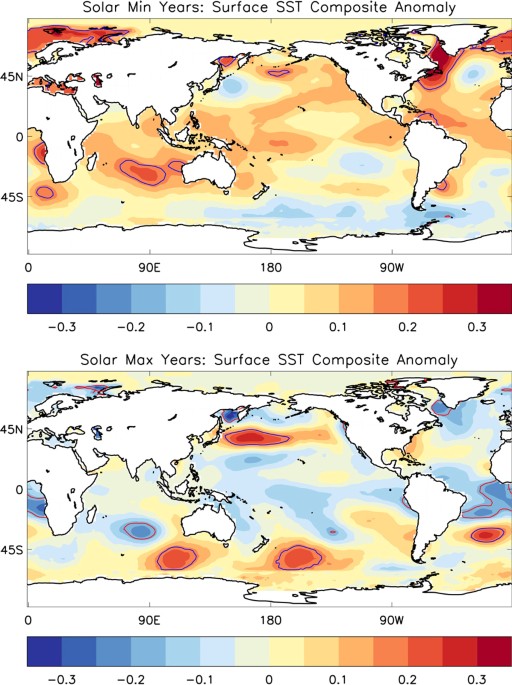
Tropical Pacific SST composites using NOAA Extended V4 (ERSST) data for solar Max (Top) and Min years (Bottom) during DJF. Levels usually significant up to 95% level are overlaid by opposite coloured contour. Plots are generated using IDL software, version 8 with the data from NOAA/OAR/ESRL PSD, Boulder, Colorado, USA, from their website at (http://www.esrl.noaa.gov/psd/).
Importantly, the analysis shows little to no solar influence upon the ENSO 3.4 ocean sector, but as the graph above shows the effect is much broader. Roy concludes that ENSO operates mostly independently of solar influence. Even more striking is the result for NH winter, showing solar minima associated with generally warmer SST and maxima generally cooler. Dr. Roy explains the solar influence in terms of two separate processes. Bottom up is fluctuations in SSTs while top-down is UV effects upon the stratosphere extending downward expressed in SLP differentials.
For a discussion of the solar/climate mechanism there is Solar cyclic variability can modulate winter Arctic climate by Indrani Roy Scientific Reportsvolume 8, Article number: 4864 (2018). Excerpts in italics with my bolds.
Abstract
This study investigates the role of the eleven-year solar cycle on the Arctic climate during 1979–2016. It reveals that during those years, when the winter solar sunspot number (SSN) falls below 1.35 standard deviations (or mean value), the Arctic warming extends from the lower troposphere to high up in the upper stratosphere and vice versa when SSN is above. The warming in the atmospheric column reflects an easterly zonal wind anomaly consistent with warm air and positive geopotential height anomalies for years with minimum SSN and vice versa for the maximum. Despite the inherent limitations of statistical techniques, three different methods – Compositing, Multiple Linear Regression and Correlation – all point to a similar modulating influence of the sun on winter Arctic climate via the pathway of Arctic Oscillation. Presenting schematics, it discusses the mechanisms of how solar cycle variability influences the Arctic climate involving the stratospheric route. Compositing also detects an opposite solar signature on Eurasian snow-cover, which is a cooling during Minimum years, while warming in maximum. It is hypothesized that the reduction of ice in the Arctic and a growth in Eurasia, in recent winters, may in part, be a result of the current weaker solar cycle.
Results
In summary, for solar Min years, the warm air column is associated with positive geopotential height anomalies and an easterly wind, which reverses during Max years. Such NAM feature is clearly evident supporting the hypothesis of communicating a solar signal to Arctic via winter NAM (North Annular Mode).
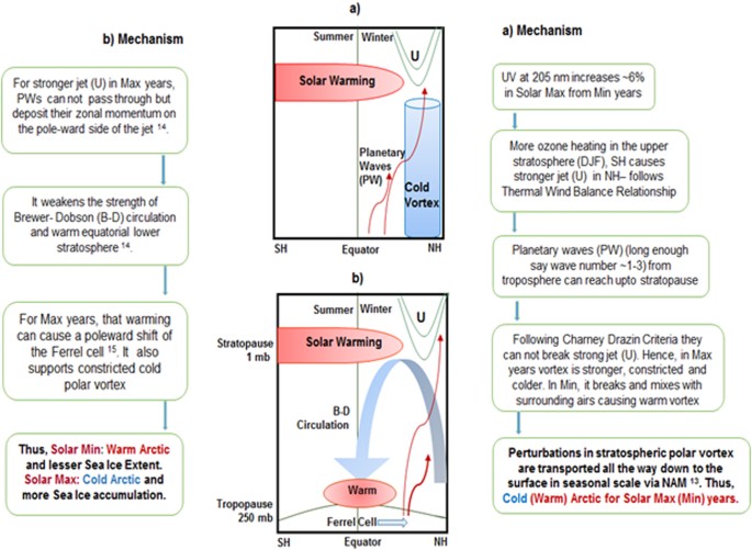
Above: Mechanism to describe the stratospheric pathway for solar cycle variability to influence the Arctic climate. Mechanisms for (a) discuss a route where perturbation in the upper stratospheric polar vortex is transported downwards and impacts the Arctic on a seasonal scale via the winter NAM (flowchart is presented on the right). Mechanisms for (b) discusses the route that involves upper stratospheric polar vortex, tropical lower stratosphere, Brewer-Dobson circulation and Ferrel cell (flowchart is presented to the left). It is created using images or clip art available from Powerpoint.
During DJF, Arctic sea ice extent suggests a strong correlation with SSN (99% significant) and even with AOD (95% significant) (Table 3a). SSN is also found to be strongly correlated with AO (95% significant). Figure 8a shows that significant correlation between Arctic sea ice extent and SSN is still present in other seasons as well. However, the correlation between SSN and AO is only significant in DJF, confirming that the possible route of solar influence on winter Arctic sea ice is via the AO. On the other hand, the influence of AO on Arctic sea ice extent is not present during winter. It is strongest during JJA, though fails to exceed a significant threshold of 95% level.
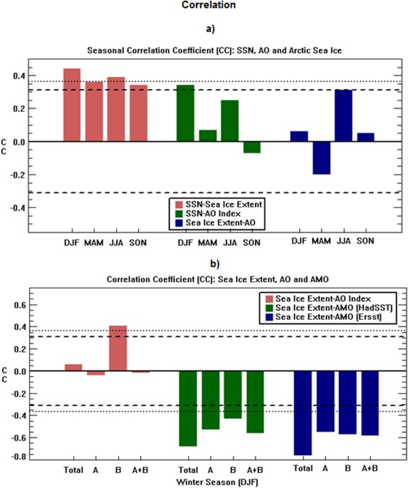
Results of Correlation Coefficient (c.c) between Sea Ice Extent and various other parameters. (a) Seasonal c.c. for four different seasons are presented using other parameters as SSN and AO, and (b) c.c. for the winter season in different regions using other parameters as AO and AMO. Significant levels of 95% and 99% using a students ‘t-test’ are marked by dashed line and dotted line respectively. Plots are prepared using IDL software, version 8.
In terms of oceanic longer-term variability, here we particularly focus on the AMO and find a strong connection between sea ice and AMO in winter, agreeing with previous studies45,46. Earlier discussions suggested that there are few differences in region A and B relating to trend (Figs S6 and S7), but correlation technique indicated a very strong anti-correlation between the winter AMO index and sea ice in all regions of our considerations (Fig. 8b)). Even using two different data sources (HadSST and ERSST) we arrive at similar results, and it is also true for overall sea ice extent. It could also be possible that, in region B, due to a strong presence of AO influence of the sun, it may mask some of the influence of the longer-term trend (seen in Fig. 2) to suggest a lesser trend, as also noted in Figs S6 and S7.
This Matters As We Reach Solar Minimum for Cycle 24
The latest observations show this solar cycle is over, perhaps the next one beginning. With no sunspots seen since June, this is unusually quiet.

The solar surface at the moment is “Spotless” and has been for a month.

Summary
The sun is the primary source of energy in the earth/atmosphere system, but the actual role of the sun and related mechanisms to support varied regional climate responses and its seasonality around the world, are still poorly understood. Solar energy output varies in cycles, of which the 11-year cyclic variability is one of the most crucial ones. It causes differences in the amount of solar energy absorbed in the UV part of the spectrum within the upper stratosphere, varying from 6 to 8%. Such variation is believed to be one of the most important solar energy outputs to influence the climate of the earth and that knowledge of cyclic behaviour can also be used for future prediction purposes. Apart from solar UV related effects on earth’s climate, studies also identified effects related to solar particle precipitation.
Various studies have also detected an influence of the El Nino Southern Oscillation (ENSO)22 and the Pacific Decadal Oscillation (PDO) on Arctic sea ice. An association between the sun and ENSO are discussed in various research. Because of related complexities along with various linear and nonlinear couplings among major modes of variability, the role of the sun on Arctic air temperatures and sea ice extent and related mechanisms remains poorly understood/explored.
While many studies point to anthropogenic influences on the long-term sea ice decline, this study is motivated by the potential links between the sun and the surface climate through stratospheric processes. Alongside warming in the Arctic, a cooling is noticed around Eurasian sector despite continuing rise of greenhouse gas concentrations. Various modelling groups, however, made unsuccessful efforts to detect an association between Eurasian cooling and Arctic sea-ice decline. In this work, we evaluate the impact of the solar 11-year cycle, measured in terms of solar sunspot number (SSN), as a driving factor to modulate Arctic and surrounding climate. The influences of SSN on various surface parameters, such as Sea Level Pressure (SLP), Sea Surface Temperature (SST), and the polar stratosphere are well recognised. If there is indeed a link between the solar cycle and Arctic climate, it is possible that the 11-year solar cycle can be used to improve seasonal and decadal predictions of sea ice. In the present study, we use a combination of observational and reanalysis datasets to uncover relationships between the sun’s variability and Arctic surface climate, via the modulation of NAM and downward propagation of anomaly from upper stratospheric winter polar vortex.
Our result suggests the latest rapid decline of sea ice around the Arctic in the recent winter decade/season could also have contributions from the current weaker solar cycle. The last 14 years are dominated by solar Min years and have only one Max. This is unlike other previous years, where the number of Max and Min years were evenly distributed (five each). The cumulative effect from the past 13 solar Min years could have played a role in the current record decline of the last winter, 2017. The current weaker solar cycle may also have contributions on increase in winter snow cover around the Eurasian sector.
Presenting schematics and flowcharts, we discussed mechanisms of how solar cycle variability influences Arctic climate. In the first route, perturbation in the upper stratospheric polar vortex is transported downwards and modulates the Arctic in a seasonal scale via the winter NAM. Another route was shown, which could involve upper stratospheric polar vortex, tropical lower stratosphere, Brewer-Dobson circulation and Ferrel cell. It could also reinforce the findings of the ‘Solar Max (Min) – cold (warm) Arctic’ scenario.
 An editorial at Investor’s Business Daily poses the question: Why Hasn’t The California Heat Wave Sparked The Usual Global Warming Hysteria? Excerpts in italics with my bolds.
It wasn’t long ago when the mainstream press took every opportunity, no matter how weak the connection, to blame bad things on global warming. So far, at least, we haven’t found one major story using the heat wave gripping the southwest to sound the alarm about global warming.
This lack of alarmism has not gone unnoticed.
Writing at the New Republic this week, Emily Atkin complained that despite record-breaking heat and a wildfire season that, she says, is already worse than usual, “there’s no climate connection to be found in much news coverage, even in historically climate-conscious outlets like NPR and The New York Times.”
When Atkin contacted NPR for an explanation, the network’s science editor said “You don’t just want to be throwing around, ‘This is due to climate change, that is due to climate change.‘”
Wow.
Also this week, Chris Hayes of the uber-liberal MSNBC responded to a complaint on Twitter that his network wasn’t clanging the global warming alarm bells loudly enough or regularly enough with this tweet:
“every single time we’ve covered it’s been a palpable ratings killer. so the incentives are not great.”
So why this sudden outburst of common sense among the mainstream press?
Perhaps they’ve come to the realization that after decades of end-of-the-world predictions and oversaturation coverage, during which time global temperatures have barely budged, the public has stopped paying attention. You can only predict the end of the world so many times, after all, before people start to get skeptical.
The attempts by scientists and environmental activists to blame everything on global warming has probably increased public skepticism as well. Case in point is a video running on the Weather Channel app about a study that claims to have found a link between suicides and climate change. Even an uninformed public will start to question the validity of all these wild claims.
The public may also have noticed that the most vocal preachers of climate change doom — Al Gore, Leonardo DiCaprio, etc. — don’t act like there’s any crisis whatsoever. They still own huge energy sucking mansions and party on massive gas guzzling yachts.
They aren’t the only global warming hypocrites. A survey earlier this year by researchers at the University of Michigan and Cornell University found that those who said they were “highly concerned” about global warming were the least likely to take individual action. Skeptics were more likely to do the things the alarmist demand: recycle, use public transportation and so forth.
How big a crisis can climate change be if those who scream the loudest about it can’t be bothered to change their own behavior?
Whatever the cause of the climate ennui, it’s clear that years of proselytizing about the “existential threat” posed by a warmer planet has failed to win many converts.
In fact, a recent Gallup survey asked people to name the most important problems facing the country today. Neither “climate change” nor “global warming” even showed up on the list of more than 45 items. Just 2% named “environment/pollution.”
We’d say the public has it right. But don’t be surprised if the media returns to its climate change obsession, if only to take a break from its Trump obsession.
Update July 28:
As if on cue the mainstream media is now awash with headlines claiming AGW is causing heat waves and forest fires.
Summary
The editors are referring to major mainstream media not rising to the bait as usual. Of course, the activist alarmist websites and blogs have been going crazy with this momentary weather situation. I noticed, however, on one of the twitter threads comments from a few climate researchers confiding that they don’t speak out lest they be branded as Alarmists.
Now that is progress if scientists are taking to heart the need to be balanced and objective conveying information. Fame and fortune may still await a breakthrough scary climate finding, but now responses will include skeptical voices. The public is not as naive and gullible as before, having been spoofed too often.

See Also: On climate polling trickery The Art of Rigging Climate Polls
And why climate and suicides do not mix Stanford Jumps Suicide Climate Shark

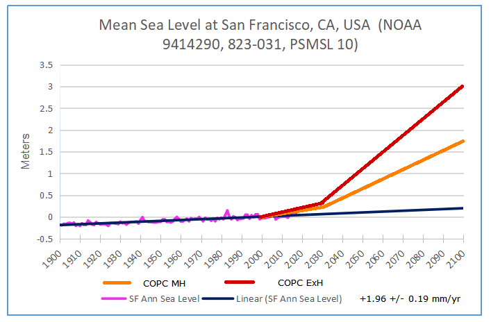
The graph displays three projections of mean sea level at San Francisco CA. The tidal gauge trend adds 0.2 meters (0.7 feet) by 2100. California Ocean Protection Council (COPC) has issued 2018 guidance on sea level rise along the California coastline. COPC takes IPCC models as gospel truth and projects future sea levels accordingly. The orange line represents COPC Medium-High risk aversion and produces 1.75 meters (5.7 feet) rise by 2100. The red line represents COPC Extremely High risk avoidance (worst case) resulting in 3.1 meters (10.2 feet) rise by 2100.
In SF Examiner is this article San Francisco studies impacts of sea level rise as state projections double Excerpts below with my bolds.
In the wake of the city’s losing lawsuit against Big Oil companies, new model projections are going for more scary numbers.
Sea level rise projections from the state Ocean Protection Council were increased earlier this year from a maximum of 66 inches to as high as 122 inches by 2100. That projection includes both sea level rise, which will account for 11 to 24 inches by 2050, and coastal erosion and shoreline flooding.
Planning Department Director John Rahaim said at a Planning Commission hearing Thursday that certain areas of The City will likely see “routine flooding” by 2030.
“Some of the numbers… are in big ranges and there’s this tendency to think of sea level rise as so far in the future that it’s hard to get people’s attention,” Rahaim said. “There are things that are happening in the short term that we really have to start thinking about. It’s not something we can put off to the next generation.”
The commission was briefed Thursday on the progress of efforts to curb the impacts of inundated shorelines since the publication of the 2016 Sea Level Rise Action Plan, which directed city agencies to assess the impacts of sea level rise on San Francisco.

State projections for how high the ocean could rise this century have as much as doubled, giving new urgency to efforts to plan for mitigation efforts, San Francisco planning officials said this week. Sea level rise projections from the state Ocean Protection Council were increased earlier this year from a maximum of 66 inches to as high as 122 inches by 2100. (Kevin N. Hume/S.F. Examiner)
“We have been working with our public infrastructure agencies to really understand, ‘What does this mean for MUNI? What does this mean for our Public Utilities Commission, for our parks?” Maggie Wenger, an adaption planner with the department. “And then what does it mean if those systems face impacts, for the people who live here, work here and come to visit.”
Preliminary findings suggest that between 17 and 84 miles of streets, 242 to 704 acres of open space, 335 acres to 1,203 acres of public land and 2 to 20 schools will be affected by flooding between 2030 and 2100.
The assessment found that roughly 6 percent of land area along San Francisco’s coastal areas is vulnerable to sea level rise.
“Not all areas in this zone are equally vulnerable,” said Wenger, adding that some are likely to see flooding impacts “in the next decades, others in the next century.”
Along with the assessment, The City is currently rolling out a its Port Seawall Earthquake Safety program and has adopted the Islais Creek Southeast/Southeast Mobility Adaptation strategy which focuses on design solutions to strengthening the area and improving the resilience of transportation assets.
A more than $400 million bond proposal to repair San Francisco’s seawall will go before San Francisco voters in November.
Here is the 2018 update document on State of California Sea-Level Rise Guidance
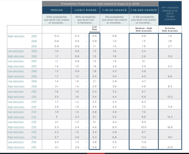
Table 1 is Projected Sea-Level Rise (in feet) for San Francisco
Probabilistic projections for the height of sea-level rise shown below, along with the H++ scenario (depicted in blue in the far right column), as seen in the Rising Seas Report. The H++ projection is a single scenario and does not have an associated likelihood of occurrence as do the probabilistic projections. Probabilistic projections are with respect to a baseline of the year 2000, or more specifically the average relative sea level over 1991 – 2009. High emissions represents RCP 8.5; low emissions represents RCP 2.6. Recommended projections for use in low, medium-high and extreme risk aversion decisions are outlined in blue boxes below.
Summary
Note that the Medium High projection adds 5 feet on top of the tidal gauge trend of 0.7 feet, a multiple of 8 times greater based upon climate models. By 2030, both COPC projections already exceed the end of century tidal gauge rise. Note also they project actual sea level rise may be only on the order of 1 or 2 feet by 2050, with rise from erosion on top. This compares to 0.3 feet estimated by 2050 from the tidal gauge including land movements.
By all means repair the sea wall to resist an additional foot or two. But the rest of it is coming from Puff the Magic Dragon.

With the nomination of Brett Kavanaugh to the Supreme Court, there is lots of speculation about what rulings might be revisited and possibly changed with his addition to the Supreme bench. One topic is the Massachusetts vs. EPA decision which gave EPA the opening to decide CO2 endangered the US population. But many do not yet grasp how flimsy and limited is the CO2 endangerment decision by EPA. As we shall see below, it was narrowly constrained to mobile sources of emissions. To extend that to stationary sources like power plants is a whole different ballgame, and one EPA is unlikely to win even if it tried. That is why the Supreme court stayed the Clean Power Plan, even with Judge Kennedy active. More detail and the technical issues are expounded below.
Robert Henneke writes a fine article in Washington Examiner Trump has a chance to rein in Obama’s out-of-control EPA Henneke is is the general counsel and director of the Center for the American Future at the Texas Public Policy Foundation. Excerpts below in italics with my bolds.
The Environmental Protection Agency has sent its replacement for the Clean Power Plan to the White House. We don’t know what’s in it (it won’t be released until the White House has a chance to review it), but we know what should be and what shouldn’t.
The new plan should restore the rule of law to an out-of-control agency. The EPA must abide by the rules set by Congress, particularly in the Clean Air Act, rather than lawlessly assuming authority it doesn’t have, as it did through the Clean Power Plan. The new plan must not repeat the mistakes of the CPP.
Carbon dioxide is the supervillain in the story of global climate change. The EPA declared even naturally-occurring CO2 as a pollutant in 2009, then sought to regulate it in the Clean Power Plan. Fortunately, the plan was stayed by the Supreme Court before it went into effect, and it remains in legal limbo.
But in December of that year, the advance notice of the new rules, the EPA indicated it would repeat some of the same mistakes of the CPP in its new guidelines.
First, EPA is not allowed to regulate greenhouse gas emissions from stationary sources (power plants) under Section 111 of the Clean Air Act. Why not? Because all emissions from such sources are already regulated under Section 112. Regulators don’t get two bites at that apple.
Congress expressly prohibited such overregulation to avoid burdensome, duplicative rules, and it required the EPA to choose only one avenue. But EPA has regulated coal-and-oil-fired electric generation unit emissions under Section 112 since 2000, and in 2012, it began regulating all fossil fuel-fired electric generation unit emissions under that section.
Second, to proceed under Section 111, the EPA is required to make an endangerment finding under the criteria for stationary sources. But there is no endangerment finding – not under the Obama administration and not now. To justify its overreach, the EPA has pointed to the endangerment finding it made in 2009 in connection with mobile source emissions (cars and trucks, etc.) under a different provision of the Clean Air Act (Section 202).
But that endangerment finding simply doesn’t apply. It doesn’t meet the criteria of Section 111, that a pollutant from stationary sources endangers the public health and welfare. Instead, it found that an aggregate of six different greenhouse gases, emitted by mobile sources, is a danger.
Why is this difference important? Section 111 permits regulation only from “a category of sources . . . [which] significantly causes or contributes significantly to air pollution [that endangers health or welfare].” This “significance” requirement is not found in Section 202.
So, the EPA would have an insurmountable task in finding that American power plants “significantly” cause or contribute to the levels of carbon dioxide thought to aggravate climate change. Carbon dioxide is ubiquitous and worldwide in scope, making any such finding fraught with peril. Given emissions of carbon dioxide worldwide, it is highly unlikely that the EPA can specifically point to greenhouse gas emissions from American power plants as a significant cause of endangerment of health or welfare.
Finally, if the EPA is to regulate carbon dioxide emissions from power plants, it must proceed under Section 108 of the Clean Air Act, not Section 111. Section 108 is the regulatory path Congress prescribed for air pollutants in the “ambient air” emitted from “numerous or diverse” sources, while Section 111 is the instrument for emissions from specific source categories that pose local pollution concerns. Carbon dioxide is the very model of a ubiquitous substance emitted into the “ambient air” from “numerous or diverse” sources. EPA cannot short-circuit the regulatory framework hard written into the Clean Air Act under section 108 by jumping to another section of the act.
The Clean Power Plan represents the worst of the regulatory abuses of the Obama administration. Its mistakes must not be repeated.
When it comes to the new plan, less is more. Texas serves as the model for success, where a deregulated electricity market has resulted in abundant energy and cleaner power plants as electricity companies adopt the latest technologies as a way to increase efficiencies and maximize profit, all while resulting in a cleaner environment.
That’s the way forward for the Clean Power Plan’s replacement.

Rannoch Moor, Scotland
Alarms are being sounded about heat waves in the Northern Hemisphere, noting heat waves in Eastern Canada and US, wildfires in N. Sweden and Siberia. The recent UK lawsuit featured the advocate claiming the Arctic is burning, so global warming is no longer in doubt. Thus UK needs to up its carbon reduction targets.
The High Court disagreed. And for good reasons not cited by the judge. The hot dry weather this summer in Siberia was preceded by extreme cold and massive snowfall, unusual winter conditions even for that climate zone. Similarly, there have been cold winters across Eurasia, while Northern Europe enjoys a BBQ summer. BTW, I recall seeing on TV May and June tennis matches in Spain where spectators were wearing jackets and head covering against the cold.
What is going on? Fact: Concurrent warm summers and cold winters are a feature of the North Atlantic climate system. It has gone on periodically throughout history, and long before humans burned fossil fuels. Below is evidence providing insight into our present experience of 2018 weather.
Concurrent Warming and Cooling
This post highlights recent interesting findings regarding past climate change in NH, Scotland in particular. The purpose of the research was to better understand how glaciers could be retreating during the Younger Dryas Stadia (YDS), one of the coldest periods in our Holocene epoch.
The lead researcher is Gordon Bromley, and the field work was done on site of the last ice fields on the highlands of Scotland. 14C dating was used to estimate time of glacial events such as vegetation colonizing these places. Bromely explains in article Shells found in Scotland rewrite our understanding of climate change at siliconrepublic. Excerpts in italics with my bolds.
By analysing ancient shells found in Scotland, the team’s data challenges the idea that the period was an abrupt return to an ice age climate in the North Atlantic, by showing that the last glaciers there were actually decaying rapidly during that period.
The shells were found in glacial deposits, and one in particular was dated as being the first organic matter to colonise the newly ice-free landscape, helping to provide a minimum age for the glacial advance. While all of these shell species are still in existence in the North Atlantic, many are extinct in Scotland, where ocean temperatures are too warm.
This means that although winters in Britain and Ireland were extremely cold, summers were a lot warmer than previously thought, more in line with the seasonal climates of central Europe.
“There’s a lot of geologic evidence of these former glaciers, including deposits of rubble bulldozed up by the ice, but their age has not been well established,” said Dr Gordon Bromley, lead author of the study, from NUI Galway’s School of Geography and Archaeology.
“It has largely been assumed that these glaciers existed during the cold Younger Dryas period, since other climate records give the impression that it was a cold time.”
He continued: “This finding is controversial and, if we are correct, it helps rewrite our understanding of how abrupt climate change impacts our maritime region, both in the past and potentially into the future.”
The recent report is Interstadial Rise and Younger Dryas Demise of Scotland’s Last Ice Fields
G. Bromley A. Putnam H. Borns Jr T. Lowell T. Sandford D. Barrell First published: 26 April 2018.(my bolds)
Abstract
Establishing the atmospheric expression of abrupt climate change during the last glacial termination is key to understanding driving mechanisms. In this paper, we present a new 14C chronology of glacier behavior during late‐glacial time from the Scottish Highlands, located close to the overturning region of the North Atlantic Ocean. Our results indicate that the last pulse of glaciation culminated between ~12.8 and ~12.6 ka, during the earliest part of the Younger Dryas stadial and as much as a millennium earlier than several recent estimates. Comparison of our results with existing minimum‐limiting 14C data also suggests that the subsequent deglaciation of Scotland was rapid and occurred during full stadial conditions in the North Atlantic. We attribute this pattern of ice recession to enhanced summertime melting, despite severely cool winters, and propose that relatively warm summers are a fundamental characteristic of North Atlantic stadials.
Plain Language Summary
Geologic data reveal that Earth is capable of abrupt, high‐magnitude changes in both temperature and precipitation that can occur well within a human lifespan. Exactly what causes these potentially catastrophic climate‐change events, however, and their likelihood in the near future, remains frustratingly unclear due to uncertainty about how they are manifested on land and in the oceans. Our study sheds new light on the terrestrial impact of so‐called “stadial” events in the North Atlantic region, a key area in abrupt climate change. We reconstructed the behavior of Scotland’s last glaciers, which served as natural thermometers, to explore past changes in summertime temperature. Stadials have long been associated with extreme cooling of the North Atlantic and adjacent Europe and the most recent, the Younger Dryas stadial, is commonly invoked as an example of what might happen due to anthropogenic global warming. In contrast, our new glacial chronology suggests that the Younger Dryas was instead characterized by glacier retreat, which is indicative of climate warming. This finding is important because, rather than being defined by severe year‐round cooling, it indicates that abrupt climate change is instead characterized by extreme seasonality in the North Atlantic region, with cold winters yet anomalously warm summers.
The complete report is behind a paywall, but a 2014 paper by Bromley discusses the evidence and analysis in reaching these conclusions. Younger Dryas deglaciation of Scotland driven by warming summers Excerpts with my bolds.
Significance: As a principal component of global heat transport, the North Atlantic Ocean also is susceptible to rapid disruptions of meridional overturning circulation and thus widely invoked as a cause of abrupt climate variability in the Northern Hemisphere. We assess the impact of one such North Atlantic cold event—the Younger Dryas Stadial—on an adjacent ice mass and show that, rather than instigating a return to glacial conditions, this abrupt climate event was characterized by deglaciation. We suggest this pattern indicates summertime warming during the Younger Dryas, potentially as a function of enhanced seasonality in the North Atlantic.
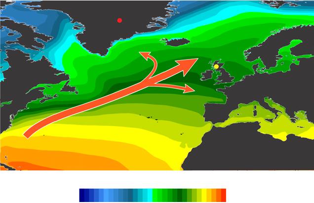
Surface temperatures range from -30C to +30C
Fig. 1. Surface temperature and heat transport in the North Atlantic Ocean. The relatively mild European climate is sustained by warm sea-surface temperatures and prevailing southwesterly airflow in the North Atlantic Ocean (NAO), with this ameliorating effect being strongest in maritime regions such as Scotland. Mean annual temperature (1979 to present) at 2 m above surface (image obtained using University of Maine Climate Reanalyzer, http://www.cci-reanalyzer.org). Locations of Rannoch Moor and the GISP2 ice core are indicated.
Thus the Scottish glacial record is ideal for reconstructing late glacial variability in North Atlantic temperature (Fig. 1). The last glacier resurgence in Scotland—the “Loch Lomond Advance” (LLA)—culminated in a ∼9,500-km2 ice cap centered over Rannoch Moor (Fig. 2A) and surrounded by smaller ice fields and cirque glaciers.
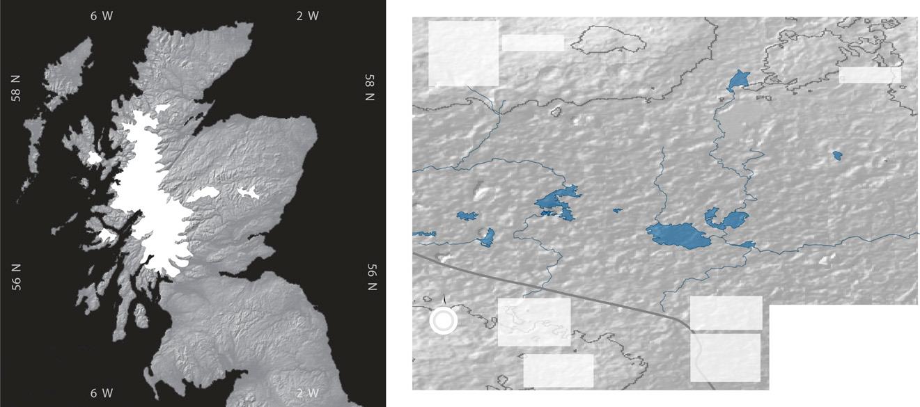
Fig. 2. Extent of the LLA ice cap in Scotland and glacial geomorphology of western Rannoch Moor. (A) Maximum extent of the ∼9,500 km2 LLA ice cap and larger satellite ice masses, indicating the central location of Rannoch Moor. Nunataks are not shown. (B) Glacial-geomorphic map of western Rannoch Moor. Distinct moraine ridges mark the northward active retreat of the glacier margin (indicated by arrow) across this sector of the moor, whereas chaotic moraines near Lochan Meall a’ Phuill (LMP) mark final stagnation of ice. Core sites are shown, including those (K1–K3) of previous investigations (14, 15).
When did the LLA itself occur? We consider two possible resolutions to the paradox of deglaciation during the YDS. First, declining precipitation over Scotland due to gradually increasing North Atlantic sea-ice extent has been invoked to explain the reported shrinkage of glaciers in the latter half of the YDS (18). However, this course of events conflicts with recent data depicting rapid, widespread imposition of winter sea-ice cover at the onset of the YDS (9), rather than progressive expansion throughout the stadial.

Loch Lomond
Furthermore, considering the gradual active retreat of LLA glaciers indicated by the geomorphic record, our chronology suggests that deglaciation began considerably earlier than the mid-YDS, when precipitation reportedly began to decline (18). Finally, our cores contain lacustrine sediments deposited throughout the latter part of the YDS, indicating that the water table was not substantially different from that of today. Indeed, some reconstructions suggest enhanced YDS precipitation in Scotland (24, 25), which is inconsistent with the explanation that precipitation starvation drove deglaciation (26).
We prefer an alternative scenario in which glacier recession was driven by summertime warming and snowline rise. We suggest that amplified seasonality, driven by greatly expanded winter sea ice, resulted in a relatively continental YDS climate for western Europe, both in winter and in summer. Although sea-ice formation prevented ocean–atmosphere heat transfer during the winter months (10), summertime melting of sea ice would have imposed an extensive freshwater cap on the ocean surface (27), resulting in a buoyancy-stratified North Atlantic. In the absence of deep vertical mixing, summertime heating would be concentrated at the ocean surface, thereby increasing both North Atlantic summer sea-surface temperatures (SSTs) and downwind air temperatures. Such a scenario is analogous to modern conditions in the Sea of Okhotsk (28) and the North Pacific Ocean (29), where buoyancy stratification maintains considerable seasonal contrasts in SSTs. Indeed, Haug et al. (30) reported higher summer SSTs in the North Pacific following the onset of stratification than previously under destratified conditions, despite the growing presence of northern ice sheets and an overall reduction in annual SST. A similar pattern is evident in a new SST record from the northeastern North Atlantic, which shows higher summer temperatures during stadial periods (e.g., Heinrich stadials 1 and 2) than during interstadials on account of amplified seasonality (30).
Our interpretation of the Rannoch Moor data, involving the summer (winter) heating (cooling) effects of a shallow North Atlantic mixed layer, reconciles full stadial conditions in the North Atlantic with YDS deglaciation in Scotland. This scenario might also account for the absence of YDS-age moraines at several higher-latitude locations (12, 36–38) and for evidence of mild summer temperatures in southern Greenland (11). Crucially, our chronology challenges the traditional view of renewed glaciation in the Northern Hemisphere during the YDS, particularly in the circum-North Atlantic, and highlights our as yet incomplete understanding of abrupt climate change.
Summary
Several things are illuminated by this study. For one thing, glaciers grow or recede because of multiple factors, not just air temperature. The study noted that glaciers require precipitation (snow) in order to grow, but also melt under warmer conditions. For background on the complexities of glacier dynamics see Glaciermania
Also, paleoclimatology relies on temperature proxies who respond to changes over multicentennial scales at best. C14 brings higher resolution to the table.
Finally, it is interesting to consider climate changing with respect to seasonality. Bromley et al. observe that during Younger Dryas, Scotland shifted from a moderate maritime climate to one with more seasonal extremes like that of inland continental regions. In that light, what should we expect from cooler SSTs in the North Atlantic?
Note also that our modern warming period has been marked by the opposite pattern. Many NH temperature records show slight summer cooling along with somewhat stronger warming in winter, the net being the modest (fearful?) warming in estimates of global annual temperatures. Then of course there are anomalous years like this one where cold winters combine with warm summer periods.
It seems that climate shifts are still events we see through a glass darkly.


Fresh evidence this week linking climate alarm and suicidal fascination. I am referring to all the mass media reports right now that climate change will cause large numbers of suicides. The claim (yet again from my alma mater Stanford) is ludicrous for many reasons:
1. A suicide is a personal event with many contributing factors, weather and climate being the most peripheral.
2. Serious suicide researchers have identified risk factors that inform caregivers, no mention of climate. Franklin et al. provide this analysis of experience with suicidal incidents Risk Factors for Suicidal Thoughts and Behaviors: A Meta-Analysis of 50 Years of Research.

With such complexity of influencing factors, putting emphasis on a bit of warming is both myopic and lopsided. For example, some places report springtime suicides are more frequent, others see more such deaths in Summer or Autumn. The seasonal relationship is quite mixed in studies with various theories being suggested along with great uncertainty.
3. Suicides occur more frequently in colder climates than in warmer ones. For example, European studies find the highest rates in eastern European nations and lowest rates in Mediterranean countries.
4. Preventing suicides is a serious issue, and has nothing to do with reducing CO2.
But the whole climate alarm movement is stained with a suicidal impulse and disdain for humanity
Micheal Walsh published The Suicidal Narrative of the Modern Environmental Left, November 16, 2017.
Walsh presents two recent experiences showing how environmental concerns are embedded everywhere including plane trips and merchandising, then gets into the implications. His text with my bolds and images.
It’s all just advertising, of course, and thus harmless enough. It also goes to reinforcing the narrative: that selfish man is the cause of species endangerment, that primitive societies are superior to developed ones (but then who would buy the locally sourced cocoa beans and moringa leaves?), and that traditional medicine—which is to say, no medicine at all—is somehow superior to what those pill-pushing quacks foist on you before they climb in their BMWs and head out to the links for a round or two of golf. Were that true, the ancient Greeks and Romans might all have lived into their 80s, instead of dying in their 20s and 30s, as unsustainable folks tended to do back then.
Which brings us, ineluctably, to “climate change” and this piece in the Times: “The More Education Republicans Have, the Less They Tend to Believe in Climate Change.” Yes, you read that right:
“Climate change divides Americans, but in an unlikely way: The more education that Democrats and Republicans have, the more their beliefs in climate change diverge. About one in four Republicans with only a high school education said they worried about climate change a great deal. But among college-educated Republicans, that figure decreases, sharply, to 8 percent.”
The author’s underlying assumption is that the more you know about “man-made climate change,” the more eager you should be to chow down on Endangered Species Chocolate or shovel some women’s-collective moringa into your smoothie before you leave your ant-farm apartment to hop on the mass-transit system on your way to a day job that somehow involves you, personally, saving the planet—not so much by what you do, but by what you don’t do.

But that’s not a future we on the Right want to embrace. I take this poll as a heartening sign that the more you educate yourself about the transparent fraud of “man-made climate change,” the less you’re likely to believe in their genteel fictions of peaceful, happy villages in Liberia or their apocalyptic notions of the End of the World as We Know It, just about any day now. As we’ve learned time and again, mountebanks and charlatans are always promising that the end of days is just around the corner, if only we will repent; find Jesus; join their cult; give away all our possessions; or at least sign up for a lifetime supply of snake oil, delivered by Amazon drones right to our doorsteps.
We’ve seen this movie before, of course. In April, Mark J. Perry of the American Enterprise Institute detailed 18 different instances when “[t]he prophets of doom were not simply wrong, but spectacularly wrong.”

Never mind that the Earth’s climate is always changing; we wouldn’t be here at all if it hadn’t. Never mind that there’s little humans can do to interfere with planetary processes, most of which are beyond our ken. Never mind that we flatter ourselves if we think so. Never mind that to characterize carbon dioxide—which we exhale so that the Amazon rain forest and those West African moringa plants might inhale—as a dangerous “greenhouse gas” is profoundly anti-human.
It’s what you’d expect from a political philosophy that denies God and sees itself as its own worst enemy: a narrative that must end in suicide, and all in the name of the greater good. All we ask our friends on the Left is not to take us with you.

Climate lemmings on the move.
More on the bogus Stanford research linking suicides to climate: Stanford Jumps Suicide Climate Shark


RAPID Array measuring North Atlantic SSTs.
For the last few years, observers have been speculating about when the North Atlantic will start the next phase shift from warm to cold.

Source: Energy and Education Canada
An example is this report in May 2015 The Atlantic is entering a cool phase that will change the world’s weather by Gerald McCarthy and Evan Haigh of the RAPID Atlantic monitoring project. Excerpts in italics with my bolds.
This is known as the Atlantic Multidecadal Oscillation (AMO), and the transition between its positive and negative phases can be very rapid. For example, Atlantic temperatures declined by 0.1ºC per decade from the 1940s to the 1970s. By comparison, global surface warming is estimated at 0.5ºC per century – a rate twice as slow.
In many parts of the world, the AMO has been linked with decade-long temperature and rainfall trends. Certainly – and perhaps obviously – the mean temperature of islands downwind of the Atlantic such as Britain and Ireland show almost exactly the same temperature fluctuations as the AMO.
Atlantic oscillations are associated with the frequency of hurricanes and droughts. When the AMO is in the warm phase, there are more hurricanes in the Atlantic and droughts in the US Midwest tend to be more frequent and prolonged. In the Pacific Northwest, a positive AMO leads to more rainfall.
A negative AMO (cooler ocean) is associated with reduced rainfall in the vulnerable Sahel region of Africa. The prolonged negative AMO was associated with the infamous Ethiopian famine in the mid-1980s. In the UK it tends to mean reduced summer rainfall – the mythical “barbeque summer”.Our results show that ocean circulation responds to the first mode of Atlantic atmospheric forcing, the North Atlantic Oscillation, through circulation changes between the subtropical and subpolar gyres – the intergyre region. This a major influence on the wind patterns and the heat transferred between the atmosphere and ocean.
The observations that we do have of the Atlantic overturning circulation over the past ten years show that it is declining. As a result, we expect the AMO is moving to a negative (colder surface waters) phase. This is consistent with observations of temperature in the North Atlantic.
Cold “blobs” in North Atlantic have been reported, but they are usually a winter phenomena. For example in April 2016, the sst anomalies looked like this

But by September, the picture changed to this

And we know from Kaplan AMO dataset, that 2016 summer SSTs were right up there with 1998 and 2010 as the highest recorded.
As the graph above suggests, this body of water is also important for tropical cyclones, since warmer water provides more energy. But those are annual averages, and I am interested in the summer pulses of warm water into the Arctic. As I have noted in my monthly HadSST3 reports, most summers since 2003 there have been warm pulses in the north atlantic.
 The AMO Index is from from Kaplan SST v2, the unaltered and untrended dataset. By definition, the data are monthly average SSTs interpolated to a 5×5 grid over the North Atlantic basically 0 to 70N. The graph shows warming began after 1992 up to 1998, with a series of matching years since. Because McCarthy refers to hints of cooling to come in the N. Atlantic, let’s take a closer look at some AMO years in the last 2 decades.
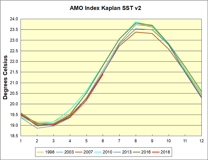
This graph shows monthly AMO temps for some important years. The Peak years were 1998, 2010 and 2016, with the latter emphasized as the most recent. The other years show lesser warming, with 2007 emphasized as the coolest in the last 20 years. Note the red 2018 line is at the bottom of all these tracks. Most recently June 2018 is 0.4C lower than June 2016.
With all the talk of AMOC slowing down and a phase shift in the North Atlantic, we await SST measurements for July, August and September to confirm if cooling is starting to set in.
