July | 2016 | Science Matters

US Students Improving Math

Posted on July 31, 2016 by Ron Clutz

Breakthrough in Math Literacy could have implications for understanding climate science.

WASHINGTON—In what experts are describing as the most marked improvement in American academic performance in decades, a study released Friday by the U.S. Department of Education has found that the majority of the nation’s students have attained the skills necessary to recognize math.

“We were encouraged to find that when presented with a series of numbers, mathematical symbols, or even fairly complex equations, more than half of our young people were able to correctly identify math as the academic subject before them,” said Undersecretary of Education Ted Mitchell, who noted that for the first time on record, over 50 percent of the country’s first- through 12th-grade students are readily able to distinguish math from other areas of study when it appeared alongside English, social studies, foreign languages, or history on a standardized test.

“While our schools should feel proud of this accomplishment, let’s remember that we must keep striving to do better. Too many Americans still graduate high school without learning to recognize any math beyond basic arithmetic, and our nation’s children still lag far behind students in other developed nations in their ability to identify geometry, algebra, and calculus as math.”

A related Education Department study found that a majority of American eighth-graders are now able to look at a map of the earth and point to where the world is.

This was a Sunday funny from the Onion

Hollywood’s Climate Fantasy

Posted on July 31, 2016 by Ron Clutz

At the DNC this week, the symbolism was perfect when Hollywood introduced a film presentation on climate change. The classic movie drama arises from one fundamental predicament: the hero confronts the villain threatening the town. It is all make-believe, as when actor Gary Cooper at high noon went out on a stage set to meet his scripted destiny, with the cameras rolling.

Of course, the retelling of the same story requires adding twists and expanded stakes, along with special effects. Now it is the global village at risk, and nature itself turning cancerous because of us. Good people want to stop the industrial poisonous machine, but evil deniers stand in the way. It is a cause for all time, to save the future for our children, and get people into the streets to make the difference.

But it is not science, it is fantasy. Nothing unusual is happening with the weather. There will be cooling as well as warming in the future, and we will need affordable reliable energy, as well as robust infrastructures, to survive and prosper. That will take sustained effort and practical, day-in, day-out attention to details. Not very dramatic stuff.

There is a word for the mental state of confusing make-believe with reality: It is called Delusion. It works as entertainment, but It is not a good frame of mind for policymakers.

Footnote:

If you have been taken in by global warming claims, you should know that temperature records show no unusual warming is occurring. (link below)

The Climate Story (Illustrated)

Climate Whack-A-Mole

Posted on July 28, 2016 by Ron Clutz

The Joys of Playing Climate Whack-A-Mole

Dealing with alarmist claims is like playing whack-a-mole. Every time you beat down one bogeyman, another one pops up in another field, and later the first one returns, needing to be confronted again. I have been playing Climate Whack-A-Mole for a while, and if you are interested, there are some hammers supplied below.

The alarmist methodology is repetitive, only the subject changes. First, create a computer model, purporting to be a physical or statistical representation of the real world. Then play with the parameters until fears are supported by the model outputs. Disregard or discount divergences from empirical observations. This pattern is described in more detail at Chameleon Climate Models

A series of posts here apply reality filters to attest climate models. The first was Temperatures According to Climate Models where both hindcasting and forecasting were seen to be flawed.

Others in the Series are:

Sea Level Rise: Just the Facts

Data vs. Models #1: Arctic Warming

Data vs. Models #2: Droughts and Floods

Data vs. Models #3: Disasters

Data vs. Models #4: Climates Changing

Climate Medicine

Climates Don’t Start Wars, People Do

Beware getting sucked into any model, climate or otherwise.

Climates Don’t Start Wars, People Do

Posted on July 26, 2016 by Ron Clutz

Once again the media are promoting a link between climate change and human conflicts. It is obvious to anyone in their right mind that wars correlate with environmental destruction. From rioting in Watts, to the wars in Iraq, or the current chaos in Syria, there’s no doubt that fighting degrades the environment big time.

What is strange here is the notion that changes in temperatures and/or rainfall cause the conflicts in the first place. The researchers that advance this claim are few in number and are hotly disputed by many others in the field, but you would not know that from the one-sided coverage in the mass media.

The Claim

Lately the fuss arises from this study: Climate, conflict, and social stability: what does the evidence say?, Hsiang, S.M. & Burke, M. Climatic Change (2014) 123: 39. doi:10.1007/s10584-013-0868-3

Hsiang and Burke (2014) examine 50 quantitative empirical studies and find a “remarkable convergence in findings” (p. 52) and “strong support for a causal association” (p. 42) between climatological changes and conflict at all scales and across all major regions of the world. A companion paper by Hsiang et al. (2013) that attempts to quantify the average effect from these studies indicates that a 1 standard deviation (σ) increase in temperature or rainfall anomaly is associated with an 11.1 % change in the risk of “intergroup conflict”.1 Assuming that future societies respond similarly to climate variability as past populations, they warn that increased rates of human conflict might represent a “large and critical impact” of climate change.

The Bigger Picture

This assertion is disputed by numerous researchers, some 26 of whom joined in a peer-reviewed comment: One effect to rule them all? A comment on climate and conflict, Buhaug, H., Nordkvelle, J., Bernauer, T. et al. Climatic Change (2014) 127: 391. doi:10.1007/s10584-014-1266-1

In contrast to Hsiang and coauthors, we find no evidence of a convergence of findings on climate variability and civil conflict. Recent studies disagree not only on the magnitude of the impact of climate variability but also on the direction of the effect. The aggregate median effect from these studies suggests that a one-standard deviation increase in temperature or loss of rainfall is associated with a 3.5 % increase in conflict risk, although the 95 % highest density area of the distribution of effects cannot exclude the possibility of large negative or positive effects. With all contemporaneous effects, the aggregate point estimate increases somewhat but remains statistically indistinguishable from zero.

To be clear, this commentary should not be taken to imply that climate has no influence on armed conflict. Rather, we argue – in line with recent scientific reviews (Adger et al. 2014; Bernauer et al. 2012; Gleditsch 2012; Klomp and Bulte 2013; Meierding 2013; Scheffran et al. 2012a,b; Theisen et al. 2013; Zografos et al. 2014) – that research to date has failed to converge on a specific and direct association between climate and violent conflict.

The Root of Climate Change Bias

The two sides have continued to publish and the issue is far from settled. Interested observers describe how serious people can disagree so frequently about such findings in climate science.

Modeling and data choices sway conclusions about climate-conflict links, Andrew M. Linke, and Frank D. W. Witmer, Institute of Behavioral Science, University of Colorado, Boulder, CO 80309-0483 here

Conclusions about the climate–conflict relationship are also contingent on the assumptions behind the respective statistical analyses. Although this simple fact is generally understood, we stress the disciplinary preferences in modeling decisions.

However, we believe that the Burke et al. finding is not a “benchmark” in the sense that it is the scientific truth or an objective reality because disciplinary-related modeling decisions, data availability and choices, and coding rules are critical in deriving robust conclusions about temperature and conflict.

After adding additional covariates (models 4 and 6), the significant temperature effect in the Burke et al. (1) model disappears, with sociopolitical variables predicting conflict more effectively than the climate variables. Furthermore, this specification provides additional insights into the between- and within-effects that vary for factors such as political exclusion and prior conflict.

Summary

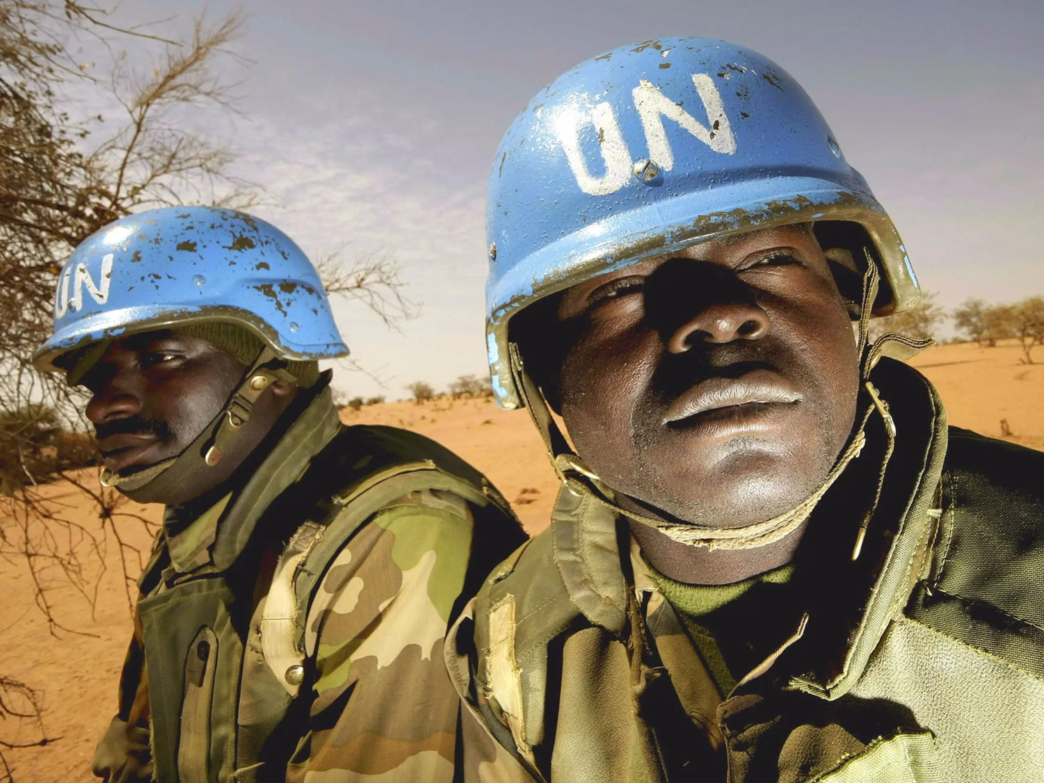
Sociopolitical variables predict conflict more effectively than climate variables. It is well established that poorer countries, such as those in Africa, are more likely to experience chronic human conflicts. It is also obvious that failing states fall into armed conflicts, being unable to govern effectively due to corruption and illegitimacy.

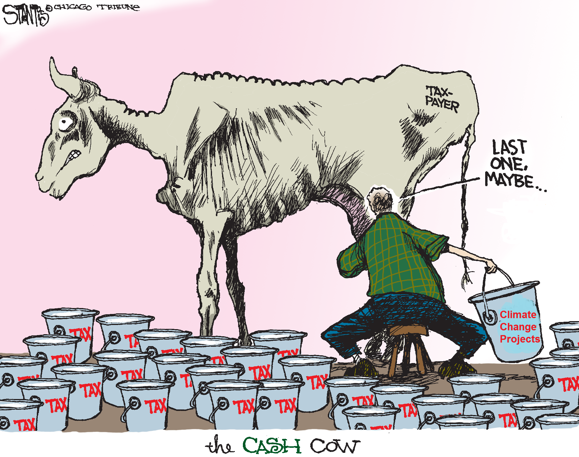
It boggles the mind that activists promote policies to deny cheap, reliable energy for such countries, perpetuating or increasing their poverty and misery, while claiming such actions reduce the chances of conflicts in the future.

Halvard Buhaug concludes (here):

Vocal actors within policy and practice contend that environmental variability and shocks, such as drought and prolonged heat waves, drive civil wars in Africa. Recently, a widely publicized scientific article appears to substantiate this claim. This paper investigates the empirical foundation for the claimed relationship in detail. Using a host of different model specifications and alternative measures of drought, heat, and civil war, the paper concludes that climate variability is a poor predictor of armed conflict. Instead, African civil wars can be explained by generic structural and contextual conditions: prevalent ethno-political exclusion, poor national economy, and the collapse of the Cold War system.

Footnote: The Joys of Playing Climate Whack-A-Mole

This post is the latest in a series here which apply reality filters to attest climate models. The first was Temperatures According to Climate Models where both hindcasting and forecasting were seen to be flawed.

Others in the Series are:

Sea Level Rise: Just the Facts

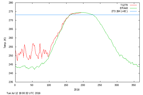
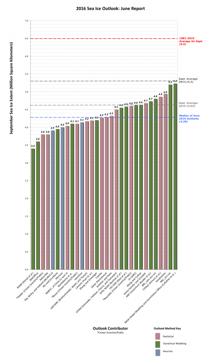
Data vs. Models #1: Arctic Warming

Data vs. Models #2: Droughts and Floods

Data vs. Models #3: Disasters

Data vs. Models #4: Climates Changing

Climate Medicine

Beware getting sucked into any model.

Climatism and Virtual Virtues

Posted on July 24, 2016 by Ron Clutz

Following an alert posted by Lubos Motl, I upgraded my windows operating system from #7 to #10, since the grace period is ending August 1. And it went quite smoothly in retrospect, but with much anxiety in the process. It seems that Windows Defender latest version doesn’t play as nice with other anti-malware programs. Also some head-scratching as to the usage of cpu by strangely named programs that may or may not be malware. And there are the inevitable hiccups and tweaks needed to restore operations as before.

It occurred to me in this process that the internet and the associated tools have become for us a kind of utility, like electricity. When we flip the light switch, the room should light up. And when we boot up our home computers, we expect to be on line and wired in. Any upgrade introduces uncertainty into that dependency, and is uncomfortable.

It also reflects on how much we modern urban dwellers exist within a cocoon of man-made structures, both physical and cyberspace. Extrapolating from our daily experience, it is a small step to thinking that the larger environment beyond our cocoons, if not entirely man-made, is at least hugely subject to human influence. And from that premise comes the climatism faith: the belief that mother Nature is being ruined by humans burning fossil fuels, that the planet will burn up, glaciers will melt, cities and islands will submerge, etc. etc. etc.

For centuries those who farm or otherwise make a living from the land or ocean have accepted and adapted to the uncertainties of weather and variable harvests. They are among the most skeptical concerning man-made climate change.

But the majority of university educated urban dwellers are converts to climatism, and participate more or less in a range of Virtual Virtues; i.e. Supporting abstract causes to protect Nature from humans. Some examples:
Save the Arctic: Support Greenpeace.:
Stop Rising CO2: Support 350.org.
Save Animals from extinction: Support WWF.
Etc.

These and other variations of “fighting Climate Change” give the illusion of “making a difference”, and thus feeling good about doing good. It is truly not about Science any more, it is about being Virtually Virtuous.

Footnote: In his lifetime, Marshall McLuhan foresaw the rise of the Global Village along with the return of tribalism, pre-conditions for the present obsession with climatism. Quotations:

“All media are extensions of some human faculty-psychic or physical.”

“The new electronic interdependence recreates the world in the image of a global village.”

“The world is now like a continually sounding tribal drum, where everybody gets the message…. all the time.”

“Our technology forces us to live mythically.”

“Politics will eventually be replaced by imagery. The politician will be only too happy to abdicate in favor of his image, because the image will be much more powerful than he could ever be.”

“The more you create village conditions, the more discontinuity and division and diversity. The global village absolutely insures maximal disagreement on all points. It never occurred to me that uniformity and tranquility were the properties of the global village. It has more spite and envy. The spaces and times are pulled out from between people. A world in which people encounter each other in depth all the time. The tribal-global village is far more divisive — full of fighting — than any nationalism ever was. Village is fission, not fusion, in depth all the time.” (McLuhan “The Hot and Cool Interview” 57–58)

That full interview is the best summary of McLuhan’s views and is here.

Climate Lemmings (h/t Beth)

Arctic Ice Outlook July 20

Posted on July 21, 2016 by Ron Clutz

For a change, note the Arctic ice chart above from AARI, the Arctic and Antarctic Research Institute, St. Petersburg, Russia. Based upon such information, they are holding up the Polar Ocean Challenge exploration ship at Murmansk because of too much ice in the Northern Sea Route. Any excessive delay puts at risk their plan to circumnavigate the North Pole counterclockwise, starting in Bristol, UK.

So what is going on with Arctic ice, and what is the outlook?

Half of the maximum ice extent is gone as of yesterday, and in a typical year, one third will remain when melting stops in September. Remember that the days are already shortening while the warming momentum will take 2 more months to cease. So 2016 started with about 15M km2 of ice, is now at 7.5M and is likely to end up about 5M km2.

The Sea Ice Prediction Network (SIPN) gathers forecasts using various methods and in June provided their first of three estimates of the September monthly average Arctic ice extent, as reported by NSIDC Sea Ice Index (produced by NOAA).

The median Outlook value for September 2016 sea ice extent is 4.28 million square kilometers with quartiles of 4.10 and 4.63 million square kilometers (See Figure 1 in the full report, below). Contributions are based on a range of methods: statistical, dynamical models, estimates based on trends, and two informal polls.

The median Outlook value is also down from last year by more than 700,000 square kilometers. This year’s forecast compares to observed values of 4.3 million square kilometers in 2007, 3.6 million square kilometers in 2012, and 4.63 million square kilometers in 2015. Only one forecast suggests a new record low is possible, one ties with 2012, while all others do not forecast a new record low for 2016. (No forecast from Peter Wadhams is included this year.)

In the chart below MASIE shows 2016 Mid-July Arctic ice extent has slipped below average and 2015. SII is back on line and was reporting similar extents during June (as it has in the past). But in July SII was showing ~400k km2 less ice most days, but is now aligned with MASIE. (SII and MASIE comparison is here.)

At the present pace of declining ice extents, 2016 is running five days ahead of the ten-year average, and seven days ahead of 2015. By the end of July, both the average and 2015 ice extents will be about 7M km2, so a loss of 1M or more in the next 10 days.

Comparing the Arctic ice extents with their maximums shows the melting is occurring mostly in the marginal seas, now including Kara Sea as expected in July.

2016202	NH Max Loss	% Loss Sea Max	% Total Loss
(0) Northern_Hemisphere	7577692	50.26%	100%
(1) Beaufort_Sea	367069	34.29%	5%
(2) Chukchi_Sea	311512	32.25%	4%
(3) East_Siberian_Sea	185840	17.09%	2%
(4) Laptev_Sea	108421	12.08%	1%
(5) Kara_Sea	808138	86.43%	10%
(6) Barents_Sea	599344	99.99%	8%
(7) Greenland_Sea	440533	66.78%	6%
(8) Baffin_Bay_Gulf_of_St._Lawrence	1451812	88.28%	18%
(9) Canadian_Archipelago	246806	28.93%	3%
(10) Hudson_Bay	1044475	82.84%	13%
(11) Central_Arctic	158032	4.87%	2%
(12) Bering_Sea	768232	100.00%	10%
(13) Baltic_Sea	97582	100.00%	1%
(14) Sea_of_Okhotsk	1308697	100.00%	17%

It is clear from the above that the bulk of ice losses are coming from Okhotsk, Barents and Bering Seas (100% melted), along with Kara Sea, Hudson Bay and Baffin Bay-St. Lawrence (67+% melted). All of them are marginal seas that will go down close to zero by September. Note: Some seas are not at max on the NH max day. Thus, totals from adding losses will vary from NH daily total.

CPC shows the Arctic Oscillation waffling between positive and negative values, recently positive and forecasted to near neutral. Generally, positive AO signifies lower pressures over Arctic ice, with more cloud, lower insolation and less melting. The outlook at this point is mixed.

September Minimum Outlook

Historically, where will ice be remaining when Arctic melting stops? Over the last 10 years, on average MASIE shows the annual minimum occurring about day 260. Of course in a given year, the daily minimum varies slightly a few days +/- from that.

For comparison, here are sea ice extents reported from 2007, 2012, 2014 and 2015 for day 260:

Arctic Regions	2007	2012	2014	2015
Central Arctic Sea	2.67	2.64	2.98	2.93
BCE	0.50	0.31	1.38	0.89
Greenland & CAA	0.56	0.41	0.55	0.46
Bits & Pieces	0.32	0.04	0.22	0.15
NH Total	4.05	3.40	5.13	4.44

Notes: Extents are in M km2. BCE region includes Beaufort, Chukchi and Eastern Siberian seas. Greenland Sea (not the ice sheet). Canadian Arctic Archipelago (CAA). Locations of the Bits and Pieces vary.

As the table shows, low NH minimums come mainly from ice losses in Central Arctic and BCE. The great 2012 cyclone hit both in order to set the recent record. The recovery since 2012 shows in 2014, with some dropoff last year, mostly in BCE.

Summary

We are well into the melt season, and the resulting minimum will depend upon the vagaries of weather between now and September. Early on, 2016 was slightly higher than 2015 in March, lower in May and now tracking slightly below the past. Note: 2016 melt season is starting without the Blob, with El Nino over, and a cold blob in the North Atlantic. The AO has been hovering around neutral, now possibly indicating cloud cover reducing the pace of melting.

Meanwhile we can watch and appreciate the beauty of the changing ice conditions.

Arctic Reflection: Clouds replace snow and ice as solar reflector NASA photo

Footnote: Regarding the colder than normal water in the North Atlantic

A 2016 article for EOS is entitled Atlantic Sea Ice Could Grow in the Next Decade

Changing ocean circulation in the North Atlantic could lead to winter sea ice coverage remaining steady and even growing in select regions.

The researchers analyzed simulations from the Community Earth System Model, modeling both atmosphere and ocean circulation. They found that decadal-scale trends in Arctic winter sea ice extent are largely explained by changes in ocean circulation rather than by large-scale external factors like anthropogenic warming.

From the Abstract of Yeager et al.

We present evidence that the extreme negative trends in Arctic winter sea-ice extent in the late 1990s were a predictable consequence of the preceding decade of persistent positive winter North Atlantic Oscillation (NAO) conditions and associated spin-up of the thermohaline circulation (THC). Initialized forecasts made with the Community Earth System Model decadal prediction system indicate that relatively low rates of North Atlantic Deep Water formation in recent years will result in a continuation of a THC spin-down that began more than a decade ago. Consequently, projected 10-year trends in winter Arctic winter sea-ice extent seem likely to be much more positive than has recently been observed, with the possibility of actual decadal growth in Atlantic sea-ice in the near future.

Arctic Ice Watch Mid-July

Posted on July 17, 2016 by Ron Clutz

In the chart below MASIE shows 2016 Mid-July Arctic ice extent has slipped below average and 2015. SII is back on line and was reporting similar extents during June (as it has in the past). But in July SII is showing ~400k km2 less ice most days. (SII and MASIE comparison is here.)

Looking into the details, some marginal seas are melting earlier than last year, while the central, enduring ice pack is relatively unaffected. Despite greater losses in Okhotsk, 2016 ice extent in June is fairly ordinary with slight differences across the regions. At the present pace of declining ice extents, 2016 is running three days ahead of the ten-year average, and seven days ahead of 2015.

US Navy predicts summer ice free Arctic by 2016. Greenpeace icebreaking ship, Arctic Sunrise, among broken floes of Arctic sea ice, photographed from the air. This image was taken in the Fram Strait. Greenpeace doing their bit to create more open water.

As the chart below shows, the seas most down from average this year are Kara, Barents, Greenland Sea and Baffin Bay. Meanwhile higher extents are showing in Chukchi, Laptev, and Hudson Bay, resulting in 2016 slightly below average. Beaufort Sea has returned to average after a weather event in June reduced ice by more than 150k km2.

Region	2016197	Day 197 Average	2016-Ave.
(0) Northern_Hemisphere	8139126	8345952	-206826
(1) Beaufort_Sea	844302	839527	4775
(2) Chukchi_Sea	698967	632572	66395
(3) East_Siberian_Sea	940706	944437	-3731
(4) Laptev_Sea	838590	592558	246032
(5) Kara_Sea	155252	371043	-215791
(6) Barents_Sea	35	54678	-54642
(7) Greenland_Sea	228393	428257	-199865
(8) Baffin_Bay_Gulf_of_St._Lawrence	201400	272271	-70872
(9) Canadian_Archipelago	684418	709717	-25299
(10) Hudson_Bay	445064	316953	128111
(11) Central_Arctic	3100876	3178016	-77140
(12) Bering_Sea	0	1600	-1600
(13) Baltic_Sea	0	2	-2
(14) Sea_of_Okhotsk	0	3125	-3125

Comparing the Arctic ice extents with their maximums shows the melting is occurring mostly in the marginal seas, now including Kara Sea as expected in July.

2016197	NH Max Loss	% Loss Sea Max	% Total Loss
(0) Northern_Hemisphere	6938473	46.02%	100%
(1) Beaufort_Sea	226143	21.13%	3%
(2) Chukchi_Sea	267022	27.64%	4%
(3) East_Siberian_Sea	146414	13.47%	2%
(4) Laptev_Sea	59220	6.60%	1%
(5) Kara_Sea	779736	83.40%	11%
(6) Barents_Sea	599344	99.99%	8%
(7) Greenland_Sea	431320	65.38%	6%
(8) Baffin_Bay_Gulf_of_St._Lawrence	1443182	87.75%	20%
(9) Canadian_Archipelago	168760	19.78%	2%
(10) Hudson_Bay	815807	64.70%	11%
(11) Central_Arctic	145834	4.49%	2%
(12) Bering_Sea	768232	100.00%	11%
(13) Baltic_Sea	97582	100.00%	1%
(14) Sea_of_Okhotsk	1308697	100.00%	18%

It is clear from the above that the bulk of ice losses are coming from Okhotsk, Barents and Bering Seas (100% melted),along with Kara Sea, Hudson Bay and Baffin Bay-St. Lawrence (65+% melted). All of them are marginal seas that will go down close to zero by September. Note: Some seas are not at max on the NH max day. Thus, totals from adding losses will vary from NH daily total.

September Minimum Outlook

For comparison, here are sea ice extents reported from 2007, 2012, 2014 and 2015 for day 260:

Arctic Regions	2007	2012	2014	2015
Central Arctic Sea	2.67	2.64	2.98	2.93
BCE	0.50	0.31	1.38	0.89
Greenland & CAA	0.56	0.41	0.55	0.46
Bits & Pieces	0.32	0.04	0.22	0.15
NH Total	4.05	3.40	5.13	4.44

Summary

We are well into the melt season, and the resulting minimum will depend upon the vagaries of weather between now and September. Early on, 2016 was slightly higher than 2015 in March, lower in May and now closing the gap. Note: 2016 melt season is starting without the Blob, with El Nino over, and a cold blob in the North Atlantic. The AO has been hovering around neutral, now possibly indicating cloud cover reducing the pace of melting.

Meanwhile we can watch and appreciate the beauty of the changing ice conditions.

Arctic Reflection: Clouds replace snow and ice as solar reflector NASA photo

Footnote: Regarding the colder than normal water in the North Atlantic

A 2016 article for EOS is entitled Atlantic Sea Ice Could Grow in the Next Decade

Changing ocean circulation in the North Atlantic could lead to winter sea ice coverage remaining steady and even growing in select regions.

From the Abstract of Yeager et al.

Climate Crisis Inc. Update

Posted on July 16, 2016 by Ron Clutz

cov_en_1 Five years ago Jo Nova provided a graphic displaying the workings of the Climate Scare Machine. The figures are out-dated and this post is to update the growth of the Climate Crisis Industry and its outlook.

From Jo Nova (here) in 2010 dollars:
Climate Change Scare Machine Cycle: see how your tax dollars are converted into alarming messages

The money, power, and influence is vastly larger on the side that benefits from the alarm
On the skeptical side, Exxon chipped in all of $23 million over ten years, but it’s chump-change. The fossil fuel industry doesn’t like carbon legislation, but it’s not life or death, unlike the situation for wind and solar, which would be virtually wiped out without the subsidies provided by the scare.

The US government has poured in $79 billion and then some. But the pro-scare funding is pervasive: for example — the Australian government spent $14 million on a single Ad campaign, and another $90 million every year on a Department of Climate Change. The UK government paid for lobbyists to lobby it, and the BBC “partners” with the lobby groups. The EU doesn’t just subsidize renewables, it also pays them to push for more subsidies. Even the dastardly Exxon paid more than 20 times as much for a single renewables research project than it did to skeptics.

Last year in carbon markets $142 billion dollars turned over, and $243 billion was invested in renewables. If the carbon market idea went global it was projected to reach $2 trillion a year. Every banker and his dog has a bone in this game. Why wouldn’t they?

Industry 2015 Update from Climate Change Business Journal

(reported in Insurance Journal here).

Interest in climate change is becoming an increasingly powerful economic driver, so much so that some see it as an industry in itself whose growth is driven in large part by policymaking.

The $1.5 trillion global “climate change industry” grew at between 17 and 24 percent annually from 2005-2008, slowing to between 4 and 6 percent following the recession with the exception of 2011’s inexplicable 15 percent growth, according to Climate Change Business Journal.

The San Diego, Calif.-based publication includes within that industry nine segments and 38 sub-segments. This encompasses sectors like renewables, green building and hybrid vehicles.

That also includes the climate change consulting market, which a recent report by the journal estimates at $1.9 billion worldwide and $890 million in the U.S.

Included in this sub-segment, which the report shows is one of the fastest growing areas of the climate change industry, are environmental consultants and engineers, risk managers, assurance, as well as legal and other professional services.

Figures for the climate change consulting market are expected to more than double in the next five years, and the report’s authors believe the climate change industry as a whole will have an even steeper and faster growth trajectory than the environmental consulting industry – an industry that in 1976 had billings of $600 million and today generates $27 billion.

Paul Driessen puts the numbers in context (here).

The answer is simple. The annual revenue of the Climate Crisis & Renewable Energy Industry has become a $1.5-trillion-a-year business! That’s equal to the annual economic activity generated by the entire US nonprofit sector, or all savings over the past ten years from consumers switching to generic drugs. By comparison, revenue for the much-vilified Koch Industries are about $115 billion, for ExxonMobil around $365 billion.

According to a 200-page analysis by the Climate Change Business Journal, this Climate Industrial Complex can be divided into nine segments:

low carbon and renewable power;
carbon capture and storage;
energy storage, such as batteries;
energy efficiency;
green buildings;
transportation;
carbon trading;
climate change adaptation; and
consulting and research.

Consulting alone is a $27-billion-per-year industry that handles “reputation management” for companies and tries to link weather events, food shortages and other problems to climate change. Research includes engineering R&D and climate studies.

In other words, the current amount of annual spending is $1.5-trillion in the two boxes of Jo Nova’s diagram: Industrials and Financial Houses. There’s additional money sloshing around in other boxes of the scare machine.

The $1.5-trillion price tag appears to exclude most of the Big Green environmentalism industry, a $13.4-billion-per-year business in the USA alone. The MacArthur Foundation just gave another $50 million to global warming alarmist groups. Ex-NY Mayor Michael Bloomberg and Chesapeake Energy gave the Sierra Club $105 million to wage war on coal (shortly before the Club began waging war on natural gas and Chesapeake Energy, in what some see as poetic justice). Warren Buffett, numerous “progressive” foundations, Vladimir Putin cronies and countless companies also give endless millions to Big Green.

Our hard-earned tax dollars are likewise only partially included in the CCBJ tally. As professor, author and columnist Larry Bell notes in his new book, Scared Witless: Prophets and profits of climate doom, the U.S. government spent over $185 billion between 2003 and 2010 on climate change items – and this wild spending spree has gotten even worse in the ensuing Obama years. We are paying for questionable to fraudulent global warming studies, climate-related technology research, loans and tax breaks for Solyndra and other companies that go bankrupt, and “climate adaptation” foreign aid to poor countries.

Also not included: the salaries and pensions of thousands of EPA, NOAA, Interior, Energy and other federal bureaucrats who devote endless hours to devising and imposing regulations for Clean Power Plans, drilling and mining bans, renewable energy installations, and countless Climate Crisis, Inc. handouts. A significant part of the $1.9 trillion per year that American businesses and families pay to comply with mountains of federal regulations is also based on climate chaos claims.

Add in the state and local equivalents of these federal programs, bureaucrats, regulations and restrictions, and we’re talking serious money. There are also consumer costs, including the far higher electricity prices families and businesses must pay, especially in states that want to prove their climate credentials.

Summary

Looking into the future, IEA expects additional spending just in the energy sector to meet climate change targets on the order of $35-trillion over the period 2015 to 2030. All this remarkable growth comes in a market for non-solutions to the non-problem of global warming. (Note to Lewandowsky: It is not a conspiracy, it’s a monopoly.)

There also may be a limit to how much can be extracted.

Footnote:

A recent example of the dash for climate cash is the rise of Climate Medicine.

Radiation Myopia

Posted on July 13, 2016 by Ron Clutz

A recent thread comment illustrates how the global warming PR campaign has installed a bogus climate paradigm in public awareness: The Supremacy of Infrared Radiation. In a discussion about clouds and the Arctic, this comment appeared:

I disagree with the comments that clouds at the poles should cause cooling.
In general the earth absorbs heat from the sun near the equator and expels it near the poles via up welling radiation. A low humidity clear sky near the poles allows most gray body radiation from the ice/oceans/land to emit directly to space. Clouds at the poles would interfere with that process and the poles would warm thus melting the ice faster. And in a general sense, that is what we’ve seen over the last 40 years. (linked to a graph of declining ice extent since 1979).

Heat Transfer Mechanisms

It takes some work to untangle the problems with this statement. Because it is true that earth’s climate system takes in solar energy mostly at the equator, which is then transported and expelled mostly at the poles. The myopia is in the notion that this is a purely radiative heat transfer. The misconception arises from confusing the view from the top of the atmosphere (TOA) with the view at the surface where we live. The TOA energy balance is purely radiative. Incoming: Short Wave (SW) in, minus Outgoing: (SW) reflected/scattered out, and minus Long Wave (LW, mostly Infrared) emitted out.

Nearer the surface, the movement of energy is dominated by other more powerful heat transfers: Conduction (from warm to cool by direct contact), Convection (air moving from warm to cool objects) and Latent Heat (water changing phases from ice to liquid to gas and back again). These processes move massive amounts of energy upward from the surface toward the nearly absolute cold of space. IR active gases, mainly H2O and the minor trace gas CO2, do absorb and re-emit some LW energy, but at a scale orders of magnitude less.

Polar Heat Exchanges

The comment above attributes warming in the Arctic to the radiative properties of H20 in clouds. There is no claim that CO2 is a factor, since it acknowledges that clear dry skies offer no significant impediment to the cooling processes. But do water vapor and clouds delay cooling in the Arctic?

While it is true that moist air in the tropics makes for mild evenings after sundown, the Arctic situation differs. There is a short season when the summer sun shines, and most of the year is dark and extremely cold.

Most people fail to appreciate the huge heat losses at the Arctic pole. Mark Brandon has an excellent post on this at his wonderful blog, Mallemaroking.

By his calculations the sensible heat loss in Arctic winter ranges 200-400 Wm2.

The annual cycle of sensible heat flux from the ocean to the atmosphere for 4 different wind speeds.

As the diagram clearly shows, except for a short time in high summer, the energy flow is from the water heating the air. Transfers by latent heat are in addition to the above.

For a long time I misinterpreted the meaning of charts like the current one below from DMI:

Those are air temperatures, and if they are above average, it means that the water is losing more heat than past normals. It’s not that warmer air causes ice melt, but the other way around: Oceans are always moving heat, and more open water means more heat loss into the air, resulting in higher air temperatures, though still way below zero most of the year.

For comparison, look at the same chart from 1977 when ice extent was much higher the entire year:

Summary

So if there is to be any warming effect on ice formation from clouds, it can only happen in peak summer, the precise time when their shading effect exceeds any radiative warming. And the existence of clouds indicates moisture in the air which came from the ocean evaporating.

The myopic focus on radiation and air temperatures leads into a false analogy: thinking the Arctic is a kind of refrigerator. I explained in some detail why this is not so: Arctic Is Not a Refrigerator

If one wants to use the refrigerator analogy in relation to earth’s climate, at least do it correctly as Dr. Salby does:

From Physics of the Atmosphere and Climate, pg.82

A closed system that performs work through a conversion of heat that is absorbed by it is a heat engine. Conversely, a system that rejects heat through a conversion of work that is performed on it is a refrigerator.

In Chap. 6, we will see that individual air parcels comprising the circulation of the troposphere behave as a heat engine. By absorbing heat at the Earth’s surface, through transfers of radiative, sensible, and latent heat, individual parcels perform net work as they evolve through a thermodynamic cycle (2.13). Ultimately realized as kinetic energy, the heat absorbed maintains the circulation against frictional dissipation. It makes the circulation of the troposphere thermally driven.

In contrast, the circulation of the stratosphere behaves as a radiative refrigerator. For motion to occur, individual air parcels must have work performed on them. The kinetic energy produced is eventually converted to heat and rejected to space through LW cooling. It makes the circulation of the stratosphere mechanically driven. Gravity waves and planetary waves that propagate upward from the troposphere are dissipated in the stratosphere. Their absorption exerts an influence on the stratosphere analogous to paddle work. By forcing motion that rearranges air, it drives the stratospheric circulation out of radiative equilibrium, which results in net LW cooling to space.

Troposphere=Heat Engine

Stratosphere = Refrigerator

Alarmist Heads in the Clouds

Posted on July 12, 2016 by Ron Clutz

A new study from Scripps at UC San Diego claims proof of greenhouse gas warming by means of changes to the clouds. The paper is behind a paywall, so the reasoning is not accessible, but the media releases will ensure wide repetition.

From the news release July 11, 2016 (here)
Clouds Are Moving Higher, Subtropical Dry Zones Expanding, According to Satellite Analysis
Scripps-led study confirms computerized climate simulations projecting effects of global warming

Inconsistent satellite imaging of clouds over the decades has been a hindrance to improving scientists’ understanding. Records of cloudiness from satellites originally designed to monitor weather are prone to spurious trends related to changes in satellite orbit, instrument calibration, degradation of sensors over time, and other factors.

When the researchers removed such artifacts from the record, the data exhibited large-scale patterns of cloud change between the 1980s and 2000s that are consistent with climate model predictions for that time period, including poleward retreat of mid-latitude storm tracks, expansion of subtropical dry zones, and increasing height of the highest cloud tops. These cloud changes enhance absorption of solar radiation by the earth and reduce emission of thermal radiation to space. This exacerbates global warming caused by increasing greenhouse gas concentrations.

The researchers drew from several independent corrected satellite records in their analysis. They concluded that the behavior of clouds they observed is consistent with a human-caused increase in greenhouse gas concentrations and a planet-wide recovery from two major volcanic eruptions, the 1982 El Chichón eruption in Mexico and the 1991 eruption of Mt. Pinatubo in the Philippines. Aerosols ejected from those eruptions had a net cooling effect on the planet for several years after they took place.

Barring another volcanic event of this sort, the scientists expect the cloud trends to continue in the future as the planet continues to warm due to increasing greenhouse gas concentrations. (My bolds)

Another Example of Lop-sided Myopia and Confirmation Bias

The report above violates basic physics, resulting in a gross distortion. Two points are critical. When it comes to clouds, the greenhouse gas that matters is H2O, not CO2. Any IR effects are 96% due to the presence of water vapor and the droplets in the clouds.

And even more importantly, as Dr. Salby illustrated (here), the net effect from clouds is cooling, not warming.

Net cloud forcing is then −15 W m−2. It represents radiative cooling of the Earth-atmosphere system. This is four times as great as the additional warming of the Earth’s surface that would be introduced by a doubling of CO2. Latent heat transfer to the atmosphere (Fig. 1.32) is 90 W m−2. It is an order of magnitude greater. Consequently, the direct radiative effect of increased CO2 would be overshadowed by even a small adjustment of convection (Sec. 8.7).

Convective clouds forming over the Amazon in a blanket smoke. Credit: Prof. Ilan Koren

This is confirmed by other researchers, such as I. Koren, G. Dagan, and O. Altaratz. From aerosol-limited to invigoration of warm convective clouds. Science, 2014; 344 (6188) here.

They then looked at another source of data: that of the Clouds’ and Earth’s Radiant Energy System (CERES) satellite instruments which measure fluxes of reflected and emitted radiation from Earth to space, to help scientists understand how the climate varies over time. When analyzed together with the aerosol loading over the same area at the same time, the outcome, says Koren, was a “textbook demonstration of the invigoration effect” of added aerosols on clouds. In other words, the radiation data fit the unique signature of clouds that were growing higher and larger. Such clouds show a strong increase in cooling due to the reflected short waves, but that effect is partly cancelled out by the enhanced, trapped, long-wave radiation coming from underneath. (My bold)

More info on clouds is here:Climate Partly Cloudy

Summary

Once again, atmospheric physics is willfully distorted in order to get a headline and burnish credentials in support of man-made climate change. They promote a myopic and lop-sided picture to frighten a public mostly ill-equipped to see through their mumbo-jumbo.

	Ron Clutz on Fed Reserve Hijacks US De…
	Multiple Choice Ques… on Multiple Choice Question re Gr…
	olesmithy on Fed Reserve Hijacks US De…
	Educating and Energi… on World of CO2 Infographics
	Educating and Energi… on The Good Old Days B.B. (Before…

Science Matters

Reading between the lines, and underneath the hype.

Month: July 2016

US Students Improving Math

Hollywood’s Climate Fantasy

Climate Whack-A-Mole

Climatism and Virtual Virtues

Arctic Ice Outlook July 20

Arctic Ice Watch Mid-July

Climate Crisis Inc. Update

Radiation Myopia

Alarmist Heads in the Clouds