2025 ended with a steadily declining rate of rising CO2 in the atmosphere following a 20 month cooling since April 2024, peak of an unusual and unexplained warming spike. That rate declined further in the first four months of 2026. Historical records show that around 1875 was the coldest time in the last 10,000 years. That was the end of the Little Ice Age (LIA), and since then temperatures have warmed at an average rate of about 0.5C per century. The recovery of the biosphere and ocean warming resulted in rising levels of CO2 in the atmosphere.

Syun-Ichi Akasofu, founder of the University of Alaska Fairbanks’ Geophysical Institute reported on this pattern in 2009.
At times, there are warming spikes, in the 1930s and 40s for example, and the rate of rising CO2 goes up. At other times, such as 1950s and 60s, temperatures cool, and rising CO2 slows down. More recently, in 2023 and 24, we saw temperatures spike up before falling back down in 2025 and now in 2026. [Note: A study of ocean biochemistry processes confirms that since the end of the LIA rising temperatures have been accompanied by rising CO2 at a rate of ~2 ppm per year. [ See: Slam Dunk: Δtemp Drives Δco2, Ocean Biochemistry at Work ]
Furthermore, going back to previous warmings prior to the satellite record shows that the entire rise of 0.8C since 1947 is due to oceanic, not human activity.

Importantly, the theory of human-caused global warming asserts that increasing CO2 in the atmosphere changes the baseline and causes systemic warming in our climate. On the contrary, all of the warming since 1947 was episodic, coming from three brief events associated with oceanic cycles. And in 2024 we saw an amazing episode with a temperature spike driven by ocean air warming in all regions, along with rising NH land temperatures, now dropping well below its peak.
Previously I have demonstrated that changes in atmospheric CO2 levels follow changes in Global Mean Temperatures (GMT) as shown by satellite measurements from University of Alabama at Huntsville (UAH). A link to that background post is provided later below.
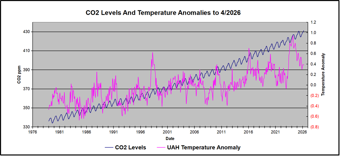
This post updates the analysis with the most current observations, testing the premise that temperature changes are predictive of changes in atmospheric CO2 concentrations. The chart at the top shows the two monthly datasets: CO2 levels in blue reported at Mauna Loa, and Global temperature anomalies in purple reported by UAHv6.1, both through April 2026. Would such a sharp increase in temperature be reflected in rising CO2 levels, according to the successful mathematical forecasting model? Would CO2 levels decline as temperatures dropped following the peak?
The answer is yes: that temperature spike resulted
in a corresponding CO2 spike as expected.
And lower CO2 levels followed the temperature decline.
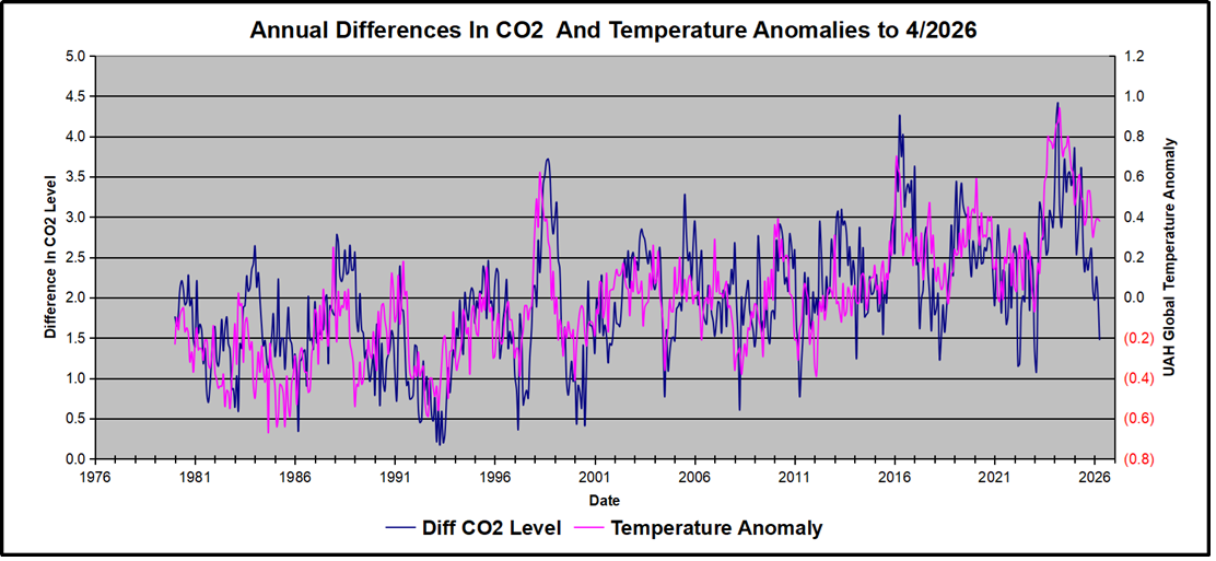
Above are UAH temperature anomalies compared to CO2 monthly changes year over year.
Changes in monthly CO2 synchronize with temperature fluctuations, which for UAH are anomalies referenced to the 1991-2020 period. CO2 differentials are calculated for the present month by subtracting the value for the same month in the previous year (for example April 2026 minus April 2025). Temp anomalies are calculated by comparing the present month with the baseline month. Note the recent CO2 upward spike and drop following the temperature spike and drop.
The table below shows clearly the pattern of observed temperatures declining along with declining rates of rising observed CO2. The CO2 rate peaked at 4.41 ppm, then declined over the next 25 months to 1.48 ppm, nearly the baseline rate since the LIA. There are fluctuations in the CO2 monthly response since the differential is influenced by the previous year as well as current year. By 2026/4, the rate of 1.48 ppm was one-third of the peak rate of 4.41 ppm.
| Month | temperature anomaly | co2 Diff. from previous year |
| 2024\1 | 0.79 | 3.32 |
| 2024\2 | 0.86 | 4.23 |
| 2024\3 | 0.87 | 4.41 |
| 2024\4 | 0.94 | 3.14 |
| 2024\5 | 0.78 | 2.87 |
| 2024\6 | 0.7 | 3.25 |
| 2024\7 | 0.74 | 3.72 |
| 2024\8 | 0.75 | 3.31 |
| 2024\9 | 0.8 | 3.53 |
| 2024\10 | 0.73 | 3.56 |
| 2024\11 | 0.64 | 3.39 |
| 2024\12 | 0.62 | 3.54 |
| 2025\1 | 0.46 | 3.85 |
| 2025\2 | 0.5 | 2.54 |
| 2025\3 | 0.58 | 2.77 |
| 2025\4 | 0.61 | 3.13 |
| 2025\5 | 0.5 | 3.61 |
| 2025\6 | 0.48 | 2.70 |
| 2025\7 | 0.36 | 2.32 |
| 2025\8 | 0.39 | 2.49 |
| 2025\9 | 0.53 | 2.34 |
| 2025\10 | 0.53 | 2.49 |
| 2025\11 | 0.43 | 2.61 |
| 2025\12 | 0.3 | 2.09 |
| 2026\1 | 0.35 | 1.97 |
| 2026\2 | 0.39 | 2.26 |
| 2026\3 | 0.38 | 2.01 |
| 2026\4 | 0.39 | 1.48 |
The final proof that CO2 follows temperature due to stimulation of natural CO2 reservoirs is demonstrated by the ability to calculate CO2 levels since 1979 with a simple mathematical formula:
For each subsequent year, the CO2 level for each month was generated
CO2 this month this year = a + b × Temp this month this year + CO2 this month last year
The values for a and b are constants applied to all monthly temps, and are chosen to scale the forecasted CO2 level for comparison with the observed value. Here is the result of those calculations.
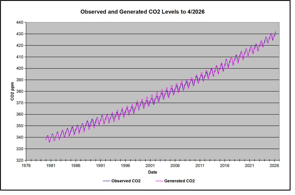
In the chart calculated CO2 levels correlate with observed CO2 levels at 0.9988 out of 1.0000. This mathematical generation of CO2 atmospheric levels is only possible if they are driven by temperature-dependent natural sources, and not by human emissions which are small in comparison, rise steadily and monotonically. For a more detailed look at the recent fluxes, here are the results since 2015, an ENSO neutral year.
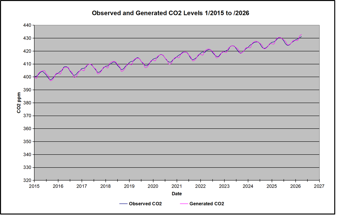
For this recent period, the calculated CO2 values match well the annual highs, while some annual generated values of CO2 are slightly higher or lower than observed at other months of the year. Still the correlation for this period is 0.9946.
Key Point
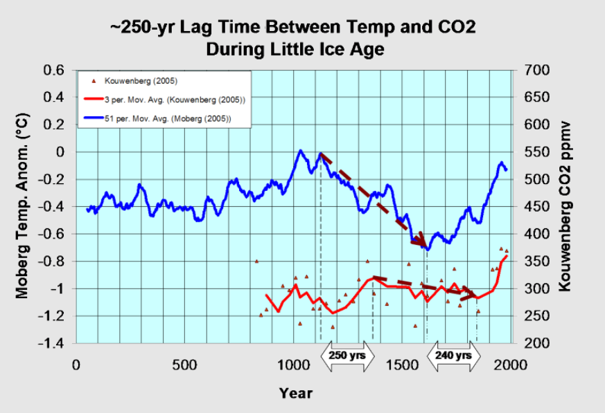
Changes in CO2 follow changes in global temperatures on all time scales, from last month’s observations to ice core datasets spanning millennia. Since CO2 is the lagging variable, it cannot logically be the cause of temperature, the leading variable. It is folly to imagine that by reducing human emissions of CO2, we can change global temperatures, which are obviously driven by other factors.

Background on Analytics and Methodology

CO2 and temperature are co-dependent variables at many levels. While the simultaneous partial differential equations can be solved to disentangle these two variables, if the uncertainty is propagated appropriately to the end result, then the uncertainty of the result is too high to be useful for example in modeling, mathematically behaving as random noise.
LikeLike
Bud, thanks for commenting and reposting this. You make a technical point about the math. But there are other independent analyses reaching the same conclusion. For example. The phase relation between atmospheric carbon dioxide and global temperature OleHumlum, KjellStordahl, Jan-ErikSolheim.
Using data series on atmospheric carbon dioxide and global temperatures we investigate the phase relation (leads/lags) between these for the period January 1980 to December 2011. Ice cores show atmospheric CO2 variations to lag behind atmospheric temperature changes on a century to millennium scale, but modern temperature is expected to lag changes in atmospheric CO2, as the atmospheric temperature increase since about 1975 generally is assumed to be caused by the modern increase in CO2.
In our analysis we used eight well-known datasets. . . We find a high degree of co-variation between all data series except 7) and 8), but with changes in CO2 always lagging changes in temperature.
Highlights
► Changes in global atmospheric CO2 are lagging 11–12 months behind changes in global sea surface temperature. ► Changes in global atmospheric CO2 are lagging 9.5–10 months behind changes in global air surface temperature. ► Changes in global atmospheric CO2 are lagging about 9 months behind changes in global lower troposphere temperature. ► Changes in ocean temperatures explain a substantial part of the observed changes in atmospheric CO2 since January 1980. ► Changes in atmospheric CO2 are not tracking changes in human emissions.
LikeLike
The math comment was meant for you. In my 46 years following this subject, lay people do not follow the math, and unfortunately too many do not follow the cause->effect sequence logic and too many think the word “significant” in science is rhetoric. My comment is attempting to point out that the math has been done, e.g. Wallace, et al, and others, to confirm the theory shown in observations such as Humlum et al. and thousands of others including you and me. Co-dependence of variables (e.g., CO2 vs surface temperature or atmospheric CO2 concentration vs CO2 estimated from fossil fuel burning) means that one form or another of statistical detrending MUST BE used or else the data can be shown to be spurious. In such cases correlation by itself without detrending is spurious.
Statistician Jamal Munshi, PhD illustrates this point elegantly in his several papers concerning CO2. If you are not familiar with these, I highly recommend them. “The method tests the relationship between two variables that share a common direction in their long term drift in time by removing the drift component and comparing the detrended series in terms of correlation at shorter intervals. When applied to atmospheric CO2, this procedure shows that the correlation between the annual rate at which anthropogenic emissions are introduced into the atmosphere and the annual rate at which CO2 accumulates in the atmosphere, though significant, does not survive into the detrended series and is therefore likely to be spurious or an artifact of the common direction of their long term drift in time to which no anthropogenic cause can be ascribed.” This is only one of many examples by Munshi: Munshi, Jamal, Responsiveness of Atmospheric CO2 to Anthropogenic Emissions: A Note (August 21, 2015). Available at SSRN: https://ssrn.com/abstract=2642639 or http://dx.doi.org/10.2139/ssrn.2642639
Second, the “airborne fraction” arguments and data are meaningless with regard to the human contribution of CO2 to the atmosphere. As you know, the so-called “airborne fraction” is the fraction of the anthropogenic carbon dioxide emission that stays in the atmosphere. Emitted carbon dioxide due to any source is partitioned according to Henry’s Law among all sinks or reservoirs. But the specific molecule emitted is usually not the same molecule that is absorbed. We exhale a CO2 molecule, or a refinery emits a CO2 molecule, but those molecules do not move great distances to be eventually absorbed at a sink. Instead, the emission causes a partial pressure wave within the atmospheric matrix that spreads out from the source and is eventually resolved by many sinks in different locations. Like an ocean wave, the water molecule moves vertically up and down but moves very little horizontally with the moving wave. In fact, the CO2 molecule emitted may never be absorbed. The carbon isotope ratio in the carbon atom in the CO2 molecule that was emitted is not the same nor correlated with the CO2 molecule that was absorbed somewhere as the partial pressure regime distributed. This is an example of the equivalency principle you described. It means that the airborne fraction and supposed lifetime of an anthropogenic sourced CO2 are useless concepts with regard to arguments about human-CO2-caused global warming or climate change.
According to Henry’s Law, if the temperature and total pressure are constant, (and the other minor natural factors pH, salinity, alkalinity are constant) then 100% of an added atmospheric trace gas will be absorbed by the environment until the phase-state equilibrium partition ratio (of the gas between liquid surface and gas phase above the surface) is restored. This holds for all natural gases and liquids in normal earth conditions. As you know ad point out, the partition ratio changes with temperature. There is a time-based variable for the rate of absorption. I and Grok illustrate in a couple of blog posts, so I won’t expand on it here.
https://budbromley.blog/2025/04/18/henrys-law-proof-experiment-for-judge-and-jury-and-scientist-with-grok-3-beta/
https://budbromley.blog/2025/09/12/second-thought-experiment-on-co2-with-grok/
I hope we will eventually have funding to do these experiments.
There are other pertinent examples. Are you familiar with the principles of gas chromatography?
LikeLike