June | 2016 | Science Matters

Brexit and the Great Divide

Posted on June 25, 2016 by Ron Clutz

Was the UK voting for Brexit a surprise? If so, it’s because we were oblivious to what has been going on with people for some time now. Lord Ashcroft’s survey shows us the UK electorate is deeply divided, but it is not primarily related to gender, generation or geography (Scotland and N. Ireland notwithstanding).

There is a cultural great divide in the UK, and elsewhere in the world that is revealed in the responses below:

By large majorities, voters who saw multiculturalism, feminism, the Green movement, globalisation and immigration as forces for good voted to remain in the EU; those who saw them as a force for ill voted by even larger majorities to leave. How the United Kingdom Voted and Why

So it is fair to say Brexit is also a repudiation of EU climate and energy policies, as explained here.

As for this phenomenon elsewhere, you must have also noticed a striking resemblance:

And the similarities extend to statements and soundbites:

There may be all kinds of reasons why I was sweating at ping-pong – but they don’t include global warming.

It is fantastic news that the world has agreed to cut pollution and help people save money, but I am sure that those global leaders were driven by a primitive fear that the present ambient warm weather is somehow caused by humanity; and that fear – as far as I understand the science – is equally without foundation. Boris Johnson (here)

We’re going to cancel the Paris agreement and stop all payment of U.S. tax dollars to global warming programs.”

“We’re going to deal with real environmental challenges, not the phony ones we’ve been hearing about. . .My priorities are very simple: clean air and clean water. Donald Trump (here)

Make no mistake: Both these gentlemen are unconventional and disruptive characters. Boris will face much resistance to his replacing Cameron. And Donald cannot be trusted to be a reliable Republican conservative, as Paul Ryan well knows.

Both are and will be denounced as “populists”, even “rabble-rousers”. Those and other such terms are always used by the elite whenever someone not in their club gains a following, becoming a political threat to those in power.

Reminder: Marx defined ideology as the set of ideas by which the ruling class maintains their power over the population. In an insightful essay (here), William Briggs sees the Brexit result as reminding us that democratic voting is inherently destablilizing. Because the hoi polloi can not be trusted to think as the establishment wants.

To the Republicans’ chagrin Trump is the one who consolidates the widespread resentment against the leftist, politically correct, authoritarian elite personified by Hilliary Clinton. In the same way Johnson was the face of the Brexit campaign victorious against the faceless EU bureaucracy.

Update June 28

Julie Burchill writes at the Spectator about the UK cultural divide, and describes the two sides as Ponces (Remainers) and Non-Ponces (Leavers). Apparently Brits use the verb “ponce” in two senses:
1. ponce around
British informal. Behave in an affected or ineffectual way:
‘I ponced around in front of the mirror’
2. ponce something up
British informal. Make overly elaborate and unnecessary changes to something in an attempt to improve it:
‘They would not let the food alone, they had to ponce it up in some way or other.’

The article is hilarious: http://blogs.spectator.co.uk/2016/06/brexit-divide-wasnt-young-old-ponces-non-ponces/

h/t American Elephants

Climate War Human Shields

Posted on June 23, 2016 by Ron Clutz

In Massachusetts, four teenagers, the Conservation Law Foundation and the Mass Energy Consumer Alliance brought the climate action case to court. “The global climate change crisis is a threat to the well being of humanity, and to my generation, that has been ignored for too long,” said one of the young prosecutors, Shamus Miller.

On Tuesday, the Massachusetts (MA) Supreme Court mandated the MA Department of Environmental Protection (DEP) to promote impactful climate legislation. The court deemed that the DEP failed to uphold climate change agreements outlined in the Global Warming Solutions Act of 2008 and “requires the department to promulgate regulations that establish volumetric limits on multiple greenhouse gas emissions sources, expressed in carbon dioxide equivalents, and that such limits must decline on an annual basis.”

This case is in accordance with “youth around the country and internationally…bringing their governments to court to secure their rights to a healthy atmosphere and stable climate,” commented Julia Olson, executive director of Our Children’s Trust (an organization that helps youth fight “game-changing” legal battles around the world).Source: Planetexperts

And who are the adults involved in Our Children’s Trust?

Supporting Experts (the usual suspects)

Dr. James Hansen
Dr. Ove Hoegh-Guldberg
Dr. Sivan Kartha
Dr. Pushker Kharecha
Dr. David Lobell
Dr. Arjun Makhijani
Dr. Jonathan Overpeck
Dr. Camille Parmeson
Dr. Stefan Rahmstorf
Dr. Steven Running
Dr. James Gustave Speth
Dr. Kevin Trenberth
Dr. Lise Van Susteren
Dr. Paul Epstein (1943-2011)
Etc

Campaign Partners (Allies whose funding depends on CO2 Hysteria)

Climate Reality Project,
Western Environmental Law Center,
Crag Law Center,
Texas Environmental Law Center,
Cottonwood Environmental Law Center,
WildEarth Guardians,
Clean Air Council,
Global Campaign for Climate Action,
Chasing Ice,
Environmental Law Alliance Worldwide,
TERRA,
Sierra Club,
350.org,
Climate Solutions,
Greenwatch,
Center for International Environmental Law..
Greenpeace
etc.

Conclusion

This is as obscene as brainwashing young Muslims to be suicide bombers. Or terrorists hiding among families to deter the drone strikes. The fact that the kids are willing is no excuse.

Think of the children! How will they feel a decade from now when they realize they have been duped and exploited by activists who figured judges would be more sympathetic to young believers?

Gifted kids

Update June 24

Some addition background in response to questions from Frederick Colbourne.

Frederick, they are employing a creative approach to the “Public Trust Doctrine”. From their website:
“Specifically, these court decisions have rejected many legal defenses raised by our opponents, including non-justiciability, standing, separation of powers and sovereign immunity. In support of our youths’ positions, and in face of argument to the contrary, the courts have validated critical climate science and reserved for the courts the exclusive right to determine whether a particular commons resource is protected by the Public Trust Doctrine for benefit of present and future generations, and whether there has been a breach of that trust. Our cases are now progressing to the next phases where the courts will make those determinations relative to our atmosphere.”

Massachusetts is ripe for this legal suit because the state passed legislation endorsing the threat of climate change and subscribing to targets for reducing emissions.

From the Court decision: “the Climate Protection and Green Economy Act, G. L. c. 21N (statute)”
“The act established a comprehensive framework to address the effects of climate change in the Commonwealth by reducing emissions to levels that scientific evidence had suggested were needed to avoid the most damaging impacts of climate change. . .In accordance with these findings, the statute requires that, by 2050, greenhouse gas emissions be reduced by at least eighty per cent below 1990 levels. G. L. c. 21N, § 3 (b).”

Note that it was Massachusetts that acted to get EPA jurisdiction over GHGs. Again from the Court decision: “See also Massachusetts v. Environmental Protection Agency, 549 U.S. 497, 505 (2007) (petition by Massachusetts, with other States, local governments, and private organizations, arguing Environmental Protection Agency abdicated responsibility under Clean Air Act to regulate emissions of four greenhouse gases, including carbon dioxide).”

This legal strategy is along the lines of “Sue and Settle” tactic employed in the past to expand the regulatory scope of the EPA. Part of this latest charade is for the state to offer a token defense so that the court requires them to do what they want to do anyways, but now armed with additional ammunition against resisters.

Note also the bait and switch: Climate change is not at issue, it is all about meeting emissions targets. It should serve also as a cautionary tale to any jurisdiction that thinks they can pass lip-service legislation and get away with politically-correct posturing.

Footnote for those not aware of Aliases for the Usual Suspects:

James “Death Trains” Hansen
Ove “Reefer Mad” Hoegh-Guldberg
Jonathan “Water Torture” Overpeck
Camille “The Extincter” Parmeson
Stefan “No Tommorow” Rahmstorf
Kevin “Hidden Heat” Trenberth

Quantifying Natural Climate Change

Posted on June 22, 2016 by Ron Clutz

Natural climate change

Recent posts have stressed the complexity of climates and their component variables. However, global warming was invented on the back of a single metric: rising global mean temperatures the last decades of last century. That was de-emphasized during the “pause” but re-emerged lately with the El-Nino-induced warming. So this post is focusing on that narrow aspect of climate change.

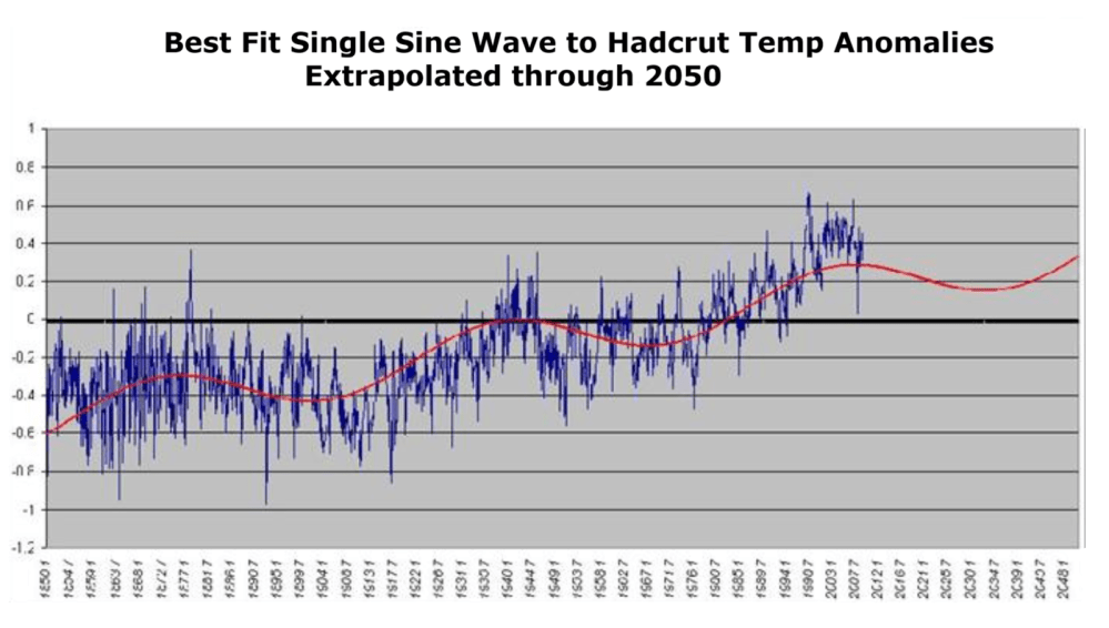
There are several papers on this blog referring to a quasi-60 year oscillation of surface temperatures due to oceanic circulations. I have also noted the attempts by many to make the link between solar activity (SA) and earth climate patterns.

Dan Pangburn is a professional engineer who has synthesized the solar and oceanic factors into a mathematical model that correlates with Average Global Temperature (AGT). On his blog is posted a monograph (here) Cause of Global Climate Change explaining clearly his thinking and the maths. I am providing some excerpts and graphs as a synopsis of his analysis, in hopes others will also access and appreciate his work on this issue.

Introduction

The basis for assessment of AGT is the first law of thermodynamics, conservation of energy, applied to the entire planet as a single entity. Much of the available data are forcings or proxies for forcings which must be integrated (mathematically as in calculus, i.e. accumulated over time) to compute energy change. Energy change divided by effective thermal capacitance is temperature change. Temperature change is expressed as anomalies which are the differences between annual averages of measured temperatures and some baseline reference temperature; usually the average over a previous multiple year time period. (Monthly anomalies, which are not used here, are referenced to previous average for the same month to account for seasonal norms.)

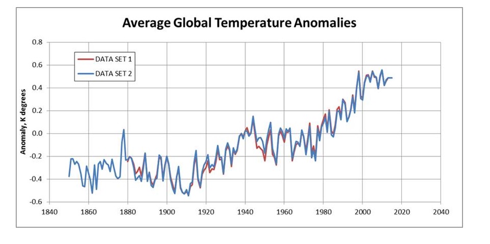
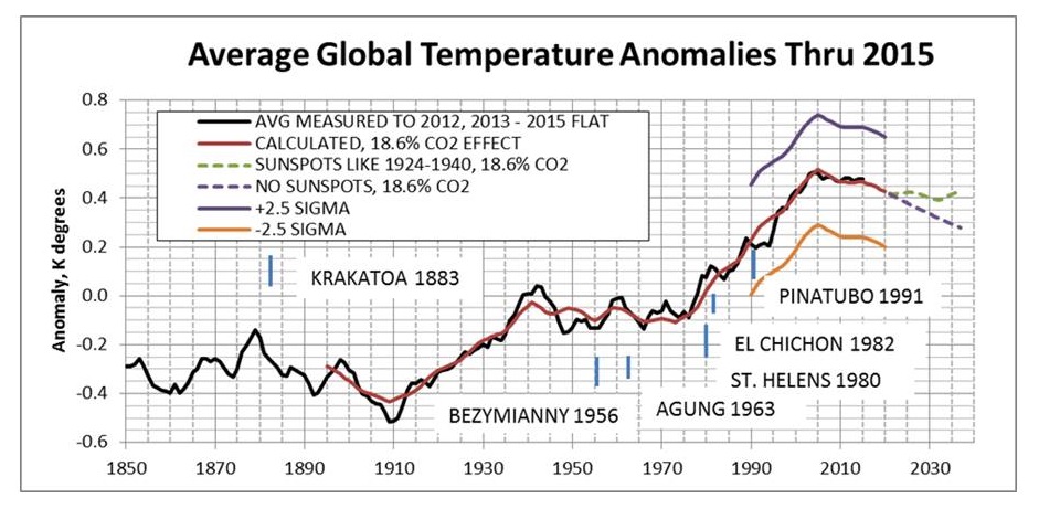
At this point, it appears reasonable to consider two temperature anomaly data sets extending through 2015. These are co-plotted on Figure 8.

1) The set used previously [12] through 2012 with extension 2013-2015 set at the average 2002-2012 (when the trend was flat) at 0.4864 K above the reference temperature. 2) Current (5/27/16) HadCRUT4 data set [13] through 2012 with 2013-2015 set at the average 2002-2012 at 0.4863 K above the reference temperature.

Accuracy of the model is determined using the Coefficient of Determination, R 2, to compare calculated AGT with measured AGT.

Oceanic Climate Impacts

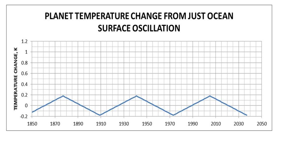
Approximation of the sea surface temperature anomaly oscillation can be described as varying linearly from –A/2 K in 1909 to approximately +A/2 K in 1941 and linearly back to the 1909 value in 1973. This cycle repeats before and after with a period of 64 years.

Figure 1: Ocean surface temperature oscillations (α-trend) do not significantly affect the bulk energy of the planet.

Comparison with PDO, ENSO and AMO

Ocean cycles are perceived to contribute to AGT in two ways: The first is the direct measurement of sea surface temperature (SST). The second is warmer SST increases atmospheric water vapor which acts as a forcing and therefore has a time-integral effect on temperature. The approximation, (A,y), accounts for both ways.

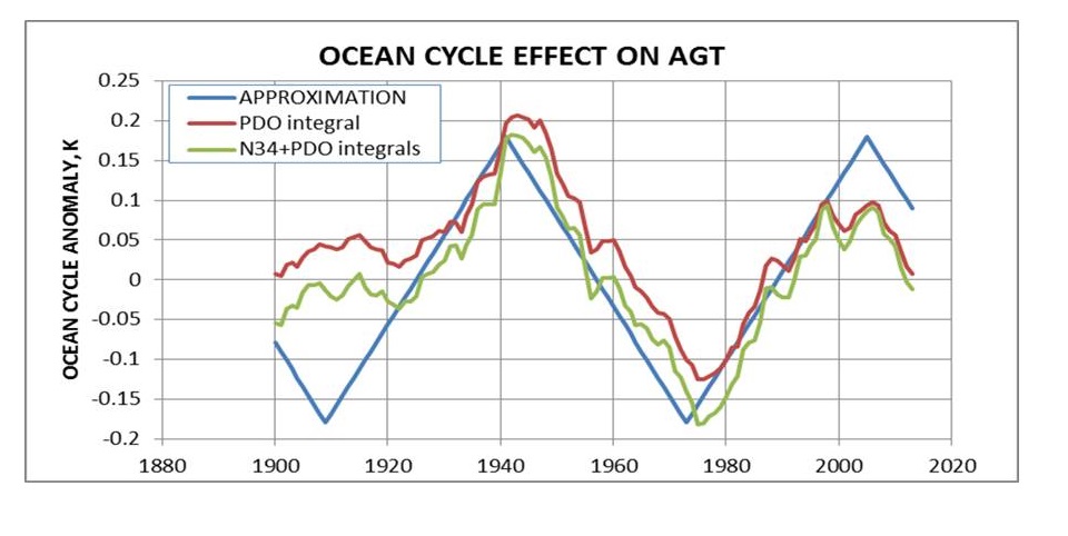
Successful accounting for oscillations is achieved for PDO and ENSO when considering these as forcings (with appropriate proxy factors) instead of direct measurements. As forcings, their influence accumulates with time. The proxy factors must be determined separately for each forcing.

Figure 2: Comparison of idealized approximation of ocean cycle effect and the calculated effect from PDO and ENSO.

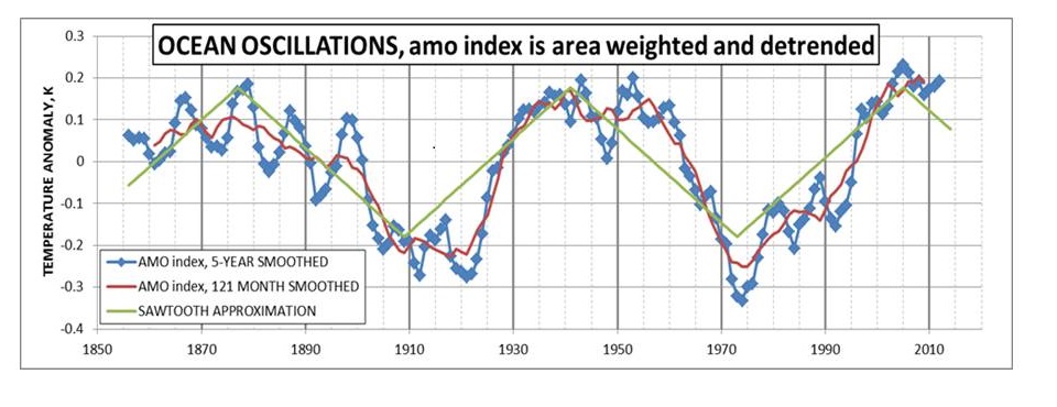
The AMO index [9] is formed from area-weighted and de-trended SST data. It is shown with two different amounts of smoothing in Figure 3 along with the saw-tooth approximation for the entire planet per Equation (2) with A = 0.36.

The high coefficients of determination in Table 1 and the comparisons in Figures 2 and 3 corroborate the assumption that the saw-tooth profile with a period of 64 years provides adequate approximation of the net effect of all named and unnamed ocean cycles in the calculated AGT anomalies.

Solar-Climate Connection

An assessment of this is that sunspots are somehow related to the net energy retained by the planet, as indicated by changes to average global temperature. Fewer sunspots are associated with cooling, and more sunspots are associated with warming. Thus the hypothesis is made that SSN are proxies for the rate at which the planet accumulates (or loses) radiant energy over time. Therefore the time-integral of the SSN anomalies is a proxy for the amount of energy retained by the planet above or below breakeven.

Also, a lower solar cycle over a longer period might result in the same increase in energy retained by the planet as a higher solar cycle over a shorter period. Both magnitude and time are accounted for by taking the time-integral of the SSN anomalies, which is simply the sum of annual mean SSN (each minus Savg) over the period of study.

The values for Savg are subject to two constraints. Initially they are determined as that which results in derived coefficients and maximum R2. However, calculated values must also result in rational values for calculated AGT at the depths of the Little Ice Age. The necessity to calculate a rational LIA AGT is a somewhat more sensitive constraint. The selected values for Savg result in calculated LIA AGT of approximately 1 K less than the recent trend which appears rational and is consistent with most LIA AGT assessments.

The sunspot number anomaly time-integral is a proxy for a primary driver of the temperature anomaly β-trend. By definition, energy change divided by effective thermal capacitance is temperature change.

Figure 10: 5-year running average of measured temperatures with calculated prior and future trends (Data Set 1) using 34 as the average daily sunspot number and with V1 SSN. R2 = 0.978887

Projections until 2020 use the expected sunspot number trend for the remainder of solar cycle 24 as provided [6] by NASA. After 2020 the ‘limiting cases’ are either assuming sunspots like from 1924 to 1940 or for the case of no sunspots which is similar to the Maunder Minimum.

Some noteworthy volcanoes and the year they occurred are also shown on Figure 9. No consistent AGT response is observed to be associated with these. Any global temperature perturbation that might have been caused by volcanoes of this size is lost in the natural fluctuation of measured temperatures.

Although the connection between AGT and the sunspot number anomaly time-integral is demonstrated, the mechanism by which this takes place remains somewhat speculative.

Various papers have been written that indicate how the solar magnetic field associated with sunspots can influence climate on earth. These papers posit that decreased sunspots are associated with decreased solar magnetic field which decreases the deflection of and therefore increases the flow of galactic cosmic rays on earth.

These papers [14,15] associated the increased low-altitude clouds with increased albedo leading to lower temperatures. Increased low altitude clouds would also result in lower average cloud altitude and therefore higher average cloud temperature. Although clouds are commonly acknowledged to increase albedo, they also radiate energy to space so increasing their temperature increases S-B radiation to space which would cause the planet to cool. Increased albedo reduces the energy received by the planet and increased radiation to space reduces the energy of the planet. Thus the two effects work together to change the AGT of the planet.

Summary

Simple analyses [17] indicate that either an increase of approximately 186 meters in average cloud altitude or a decrease of average albedo from 0.3 to the very slightly reduced value of 0.2928 would account for all of the 20th century increase in AGT of 0.74 K. Because the cloud effects work together and part of the temperature change is due to ocean oscillation (low in 1901, 0.2114 higher in 2000), substantially less cloud change would suffice.

All of this leaves little warming left to attribute to rising CO2. Pangburn estimates CO2 forcing could be at most 18.6% or 0.23C added since 1895. Given uncertainties in proxies from the past, the estimate could be as low as 0.05C, and the correlation with natural factors would still be .97 R2.

However, all is not lost for CO2. It is still an important player in the atmosphere, despite its impotence as a warming agent.

Think Global Act Local, or Not

Posted on June 21, 2016 by Ron Clutz

The slogan “Think Global, Act Local” began with multinational corporations realizing that national and regional markets around the world had distinct needs and preferences requiring accommodations. As the name implies it refers to the corporate strategy by which a global viewpoint is adopted in terms of formulating company vision, long-term aims and objectives and devising effective programs to achieve these aims and objectives, however, adaptations are made in each market according to the culture and specifications of any specific market.

Environmental activists took the notion on board during the first wave becoming aware of globalization. Early bearers of the catchphrase were for the most part supporters of an environmental movement that supported individual activism. The theory behind the saying was that in order to make large-scale global movements stick, the responsibility lay on individuals to carry out progressive practices – like environmental stewardship – in their own homes. The globe had become the new frame of reference for some far-thinking activists.

Clearly “climate change” activism operates in this mode. But as we shall see in this essay, the top-down, Global-Local approach to understanding climate and weather leads to distortions and misconceptions. In fact, climate science itself is best served by observing and establishing principles from the bottom up.

It turns out that the climate system is one of those things where averages do not tell very much, and can be misleading. For example:

Look at precipitation around the world

About 1 meter a year is the nominal average of all rain over all surfaces. Some places get up to 10 meters of rain (about 400 inches ) and others get near none. 47% of the earth is considered dryland, defined as anyplace where the rate of evaporation/transpiration exceeds the rate of precipitation. A desert is defined as a dryland with less than 25 cm of precipitation. In the image above, polar deserts are remarkably defined. It just does not have much hope of precipitation as there is little heat to move the water. More heat in, more water movement. Less heat in, less water movement.

Then there’s the seasonal patterns. The band of maximum rains moves with the sun: More north in June, more south in December. More sun, more heating, more rain. Movement in sync with the sun, little time delay. Equatorial max solar heat has max rains. Polar zones minimal heating, minimal precipitation. It’s a very tightly coupled system with low time lags.

Then Look at Temperatures

Average temperatures in F at sea level by longitude and latitude. Source: Lyndon State College Meteorology

Notice:

latitudinal change
N.H. – difference between land and ocean
U.S. west coast (upwelling and cold current) v.s. U.S. east coast (gulf stream)
influence of gulf stream in north Atlantic
highest temps are in the subtropical N.H. desert regions
west coast of S. America is cool while the east coast is warm, due to the ocean currents
much less variability in the zonal direction in the S. H.

And look at clouds and their radiative effects

The large opacity of cloud increases the optical depth of the atmosphere, introducing warming in the LW energy budget. This warming varies with cloud-top temperature and height. For SW radiation, the high reflectivity of cloud decreases the incoming solar flux, favoring reduced surface temperature. Cloud routinely covers about 50% of the Earth. It accounts for about half of the Earth’s albedo (eg, for ∼0.15). Source: Salby 2012 pg315

Globally averaged values of CLW and CSW are about 30 and −45 W m−2, respectively. Net cloud forcing is then −15 W m−2. It represents radiative cooling of the Earth-atmosphere system. This is four times as great as the additional warming of the Earth’s surface that would be introduced by a doubling of CO2.

But clearly during Northern winter (diagrams above), that net cooling occurs largely over the Southern Ocean around Antarctica.

What happens when you average all this diversity?

We have all seen graphs showing how climate models project unrealistic global mean temperatures higher than those measured by stations or satellites. But Dr. Salby in his textbook points to a more fundamental failing of the climate simulations. By construction they balance global average energy budgets, but regional realities are grossly distorted.

From IPCC Working Group 1 AR4

Figure 8.4. Root-mean-square (RMS) model error, as a function of latitude, in simulation of (a) outgoing SW radiation reflected to space and (b) outgoing LW radiation. The RMS error is calculated over all longitudes and over all 12 months of a climatology formed from several years of data. . .The Earth Radiation Budget Experiment (ERBE; Barkstrom et al., 1989) observational estimates used here are for the period 1985 to 1989 from satellite-based radiometers, and the model results are for the same period in the 20th-century simulations in the MMD at PCMDI.

Symbolizing the local energy budget is net radiation (Fig. 1.34c), which represents the local imbalance between the SW and LW fluxes F0 and F ↑(0) in the TOA energy budget (8.82). Local values of those fluxes have been measured around the Earth by the three satellites of ERBE. The observed fluxes, averaged over time, have then been compared against coincident fluxes from climate simulations, likewise averaged. Figure 8.34 plots, for several GCMs, the rms error in simulated fluxes, which have been referenced against those observed by ERBE.

Values represent the regional error in the (time-mean) TOA energy budget. The error in reflected SW flux, Fs 4 − F0 in the global mean (8.82), is of order 20 Wm−2 (Fig. 8.34a). Such error prevails at most latitudes. Differences in error between models (an indication of intermodel discrepancies) are almost as large, 10–20 Wm−2. The picture is much the same for outgoing LW flux (Fig. 8.34b). For F ↑(0), the rms error is of order 10–15 Wm−2. It is larger for all models in the tropics, where the error exceeds 20 Wm−2. . .Consequently, the simulated change introduced by increased CO2 (2–4 Wm−2), even inclusive of feedback, is overshadowed by error in the simulated change of major absorbers.

By construction, GCMs achieve global-mean energy balance. How faithfully the energy budget is represented locally, however, is another matter. The local energy budget forces regional climate, along with the gamut of weather phenomena that derive from it. This driver of regional conditions is determined internally – through the simulation of local heat flux, water vapor, and cloud. (My bold)

Conclusion

A common expression is: “The devil is in the details.” When it comes to climate, it is truer to say that we humans are bedeviled (thwarted) by nature’s details refusing to fit into our global generalities. The proper role of science is to investigate those details and revise our mental constructs.

“Global Climate” is an oxymoron.
(oxymoron: A figure of speech in which two words with opposing meanings are used together intentionally for effect; IOW a contradiction in terms. From the Greek: pointed foolishness).

Climates are plural, not global, as the Koppen system makes clear. There are hundreds of regional climate zones defined empirically by temperature and precipitation patterns. And the observational data shows those zones are highly stable; that is, fears of climate change rarely appear in any actual climates showing shifting boundaries. See post: Data vs. Models 4: Climates Changing

Thus, we are better advised to:

Think Local Climates,
Prepare Local Adaptations
for the range of future weather consequences.

Fearless Physics from Dr. Salby

Posted on June 18, 2016 by Ron Clutz

“Fearless Felix” Baumgartner ascended to the stratosphere and stepped into the void from 24.2 miles above the Earth. His speed during the fall reached Mach 1.24, and the Austrian adventurer nailed the landing. October 14, 2012 Wired

Introduction
Murry Salby is also totally committed to the atmosphere. He is a scientist with such deep and broad knowledge of atmospheric physics that he has written multiple textbooks on the subject. And yet he is not fearful for the future of our climate system, in contrast to many of his colleagues. By stepping away from “consensus” climate alarms, he has shown unusual courage by speaking plainly about the atmosphere and climate, despite attempts to silence him.

Dr. Salby’s latest textbook is entitled Physics of the Atmosphere and Climate (here). I got a copy and have been reading in it to understand where he comes down on various issues related to climate change. In particular I wanted to know what explains his divergence from IPCC climate scientists.
H/T to Kenneth Richard and No Tricks Zone

Synopsis

In reading the textbook, I find two main reasons why Salby is skeptical of AGW (anthropogenic global warming) alarm. This knowledgeable book is an antidote to myopic and lop-sided understandings of our climate system.

CO2 Alarm is Myopic: Claiming CO2 causes dangerous global warming is too simplistic. CO2 is but one factor among many other forces and processes interacting to make weather and climate.

Myopia is a failure of perception by focusing on one near thing to the exclusion of the other realities present, thus missing the big picture. For example: “Not seeing the forest for the trees.” AKA “tunnel vision.”

2. CO2 Alarm is Lopsided: CO2 forcing is too small to have the overblown effect claimed for it. Other factors are orders of magnitude larger than the potential of CO2 to influence the climate system.

Lopsided

Lop-sided refers to a failure in judging values, whereby someone lacking in sense of proportion, places great weight on a factor which actually has a minor influence compared to other forces. For example: “Making a mountain out of a mole hill.”

Overview

Salby’s textbook presents all of the physical complexity of the climate system in contrast to simplistic global warming theory. And he provides his sense of the Scales of the various processes, balancing any lopsided overemphasis on CO2 effects.

From the Preface:
Despite technological advances in observing the Earth-atmosphere system and in computing power, strides in predicting its evolution reliably – on climatic time scales and with regional detail – have been limited. The pace of progress reflects the interdisciplinary demands of the subject. Reliable simulation, adequate to reproduce the observed record of climate variation, requires a grasp of mechanisms from different disciplines and of how those mechanisms are interwoven in the Earth-atmosphere system.

What is today labeled climate science includes everything from archeology of the Earth to superficial statistics and a spate of social issues. Yet, many who embrace the label have little more than a veneer of insight into the physical processes that actually control the Earth-atmosphere system, let alone what is necessary to simulate its evolution reliably. Without such insight and its application to resolve major uncertainties, genuine progress is unlikely.

The atmosphere is the heart of the climate system, driven through interaction with the sun, continents, and ocean. It is the one component that is comprehensively observed. For this reason, the atmosphere is the central feature against which climate simulations must ultimately be validated.

The treatment focuses upon physical concepts, which are developed from first principles. It integrates five major themes:
1. Atmospheric Thermodynamics;
2. Hydrostatic Equilibrium and Stability;
3. Radiation, Cloud, and Aerosol;
4. Atmospheric Dynamics and the General Circulation;
5. Interaction with the Ocean and Stratosphere.

Lessons from Dr. Salby: Essential Elements of a Balanced Climate Understanding

Below I show some of the written statements from the textbook to illustrate how his knowledge counteracts myopic and lopsided thinking.

Focusing on CO2 from burning fossil fuels is myopic: A multitude of natural sources drive atmospheric concentrations.

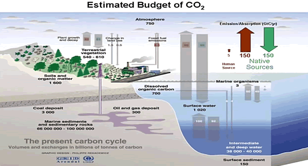
Plate 24 Estimated global carbon cycle, illustrating stores of carbon,
in GtC, and transfers in GtC/yr, where 1 GtC=109 tons of carbon.
Source: Design by Philippe Rekacewicz, UNEP/GRID-Arendal (11.07.10).

Pg.545-6
The storage of CO2 is illustrated in Fig. 17.11. Except for deep sedimentary rock, which is sequestered, most of the carbon is stored in the ocean. It accounts for some 40,000 gigatons (1012 kg) of carbon (GtC), in the form of dissolved CO2 and organic matter. Most resides in the deep ocean, where cold water supports the greatest observed concentrations. There, dissolved CO2 is controlled by the thermohaline circulation. Land and the adjoining biosphere account for only about 2000 GtC. The atmosphere contains less than 1000 GtC, concentrated in CO2. Hence, the store of carbon in the ocean is two orders of magnitude greater than the store in the atmosphere.

Equally significant are transfers of carbon into and out of the ocean. Of order 100 GtC/yr, they exceed those into and out of land. Together, emission from ocean and land sources (∼150 GtC/yr) is two orders of magnitude greater than CO2 emission from combustion of fossil fuel. These natural sources are offset by natural sinks, of comparable strength. However, because they are so much stronger, even a minor imbalance between natural sources and sinks can overshadow the anthropogenic component of CO2 emission (cf Secs 1.6.2, 8.7.1).

The values in Fig. 17.11 can be used to estimate the effective turnover time of atmospheric CO2. At an absorption rate of 100 GtC/yr, the ocean will absorb the atmospheric store of CO2 of 1000 GtC in about a decade. That absorption of CO2, which is concentrated in cold SST at polar latitudes, is nearly offset by emission of CO2 from warm SST at tropical latitudes. Warming of SST (by any mechanism) will increase the outgassing of CO2 while reducing its absorption. Owing to the magnitude of transfers with the ocean, even a minor increase of SST can lead to increased emission of CO2 that rivals other sources (Sec. 8.7.1). Further, if the increase of SST involves heat transfer with the deep ocean, the time for equilibrium to be reestablished would be centuries (Sec. 17.1.2).

Attributing rising temperatures to fossil fuels is lop-sided: Natural sinks respond to warming by releasing CO2 in far greater quantities.

Net emission rate of CO2, r˙ CO2 = d dt rCO2 (ppmv/yr), derived from the Mauna Loa record (Fig. 1.15), lowpass filtered to changes that occur on time scales longer than 2 years (solid). Superimposed is the satellite record of anomalous Global Mean Temperature (Fig. 1.39), lowpass filtered likewise and scaled by 0.225 (dashed). Trend in GMT over 1979–2009 (not included) is ∼0.125 K/decade.

Pg.65ff
Net emission of CO2 closely tracks the evolution of GMT. Achieving a correlation of 0.80, the variation of GMT accounts for most of the variance in CO2 emission.

Plotted in Fig. 1.43b is the rate of change in isotopic composition, d dt δ13C = ˙ δ13C (solid).12 Its mean is negative, consistent with the long-term decline of δ13C in ice cores (Fig. 1.14). However, like emission of CO2, differential emission of 13CO2 varies substantially from one year to the next. It too tracks the evolution of GMT – just out of phase. When GMT increases, emission of 13CO2 decreases and vice versa. The records achieve a correlation of −0.86. Hence the variation of GMT, which accounts for most of the variance in emission of CO2, also accounts for most of the variance in differential emission of 13CO2.

The out-of-phase relationship between rCO2 and δ13C in the instrumental record (Fig. 1.43) is the same one evidenced on longer time scales by ice cores (Fig. 1.14). The out-of-phase relationship in ice cores is regarded as a signature of anthropogenic emission, subject to uncertainties (Sec. 1.2.4). The out-of-phase relationship in the instrumental record, however, is clearly not anthropogenic. Swings of GMT following the eruption of Pinatubo and during the 1997–1998 El Nino were introduced through natural mechanisms (cf. Figs 1.27; 17.19, 17.20). Changes in Fig. 1.43 reveal that net emission of CO2, although 13C lean, is accelerated by increased surface temperature. Outgassing from ocean, which increases with temperature (Sec. 17.3), is consistent with the observed relationship – if the source region has anomalously low δ13C. So is the decomposition of organic matter derived from vegetation. Having δ13C comparable to that of fossil fuel, its decomposition is likewise accelerated by increased surface temperature.

Focusing on CO2 as the greenhouse gas of concern is both myopic and lop-sided: H20 makes 98% of the IR radiative activity in the atmosphere.

Pg. 47
The radiative-equilibrium surface temperature Ts is significantly warmer than that in the absence of an atmosphere.

The discrepancy between Ts and Te follows from the different ways the atmosphere processes SW and LW radiation. Although nearly transparent to SW radiation (wavelengths λ ∼ 0.5 μm), the atmosphere is almost opaque to LW radiation (λ ∼ 10 μm) that is re-emitted by the Earth’s surface. For this reason, SW radiation passes relatively freely to the Earth’s surface, where it can be absorbed. However, LW radiation emitted by the Earth’s surface is captured by the overlying air, chiefly by the major LW absorbers: water vapor and cloud. Energy absorbed in an atmospheric layer is reemitted, half upward and half back downward. The upwelling re-emitted radiation is absorbed again in overlying layers, which subsequently re-emit that energy in similar fashion. This process is repeated until LW energy is eventually radiated beyond all absorbing components of the atmosphere and rejected to space. By inhibiting the transfer of energy from the Earth’s surface, repeated absorption and emission by intermediate layers of the atmosphere traps LW energy, elevating surface temperature over what it would be in the absence of an atmosphere.

Pg. 247ff
The residual, +1.5 Wm−2, represents net warming. It is about 0.5% of the 327 Wm−2 of overall downwelling LW radiation that warms the Earth’s surface (Fig. 1.32). The vast majority of that warming is contributed by water vapor. Together with cloud, it accounts for 98% of the greenhouse effect. How water vapor has changed in relation to changes of the comparatively minor anthropogenic species (Fig. 8.30) is not known. The additional surface warming introduced by anthropogenic increases in greenhouse gases amounts to about 75% of that which would be introduced by a doubling of CO2. Arrhenius’ estimate of 5–6◦ K for the accompanying increase of surface temperature (Sec. 1.2.4) then translates into ∼4◦ K. Yet, the observed change of global-mean temperature since the mid nineteenth century is only about 1◦ K (Sec. 1.6.1). The discrepancy points to changes of the Earth-atmosphere system (notably, involving the major absorbers, water vapor and cloud) that develop in response to imposed perturbations, like anthropogenic emission of CO2.

Focusing on CO2 radiative activity is myopic: The tropospheric heat engine comprises many powerful heat transfer processes.

Figure 9.40 Cloud radiative forcing during northern winter derived from ERBE measurements on board the satellites ERBS and NOAA-9 for the (a) LW energy budget, (b) SW energy budget, and (c) net radiative energy budget. Courtesy of D. Hartmann (U. Washington).

Pg. 318ff
A quantitative description of how cloud figures in the global energy budget is complicated by its dependence on microphysical properties and interactions with the surface. These complications are circumvented by comparing radiative fluxes at TOA under cloudy vs clear-sky conditions. Over a given region, the column-integrated radiative heating rate must equal the difference between the energy flux absorbed and that emitted to space.

The components of cloud forcing (9.53) can be evaluated directly from broadband fluxes of outgoing LW and SW radiation that are measured by satellite. Figure 9.40 shows time-averaged distributions of CSW , CLW , and C. Longwave forcing (Fig. 9.40a) is large in centers of deep convection over tropical Africa, South America, and the maritime continent, where CLW approaches 100 W m−2 (cf. Fig. 1.30b). Secondary maxima appear in the maritime ITCZ and in the North Pacific and North Atlantic storm tracks (Sec. 1.2.5). Shortwave forcing (Fig. 9.40b) is strong in the same regions, where CSW < −100 W m−2. Negative SW forcing is also strong over extensive marine stratocumulus in the eastern oceans and over the Southern Ocean, coincident with the storm track of the Southern Hemisphere. Inside the centers of deep tropical convection, SW and LW cloud forcing nearly cancel. They leave small values of C throughout the tropics (Fig. 9.40c). Negative CSW in the storm tracks and over marine stratocumulus then dominates positive CLW , especially over the Southern Ocean. It prevails in the global-mean cloud forcing. Globally averaged values of CLW and CSW are about 30 and −45 W m−2, respectively.

Net cloud forcing is then −15 W m−2. It represents radiative cooling of the Earth-atmosphere system. This is four times as great as the additional warming of the Earth’s surface that would be introduced by a doubling of CO2. Latent heat transfer to the atmosphere (Fig. 1.32) is 90 W m−2. It is an order of magnitude greater. Consequently, the direct radiative effect of increased CO2 would be overshadowed by even a small adjustment of convection (Sec. 8.7).

Trusting climate models driven by CO2 sensitivity is lop-sided: Natural climate factors are poorly quantified but are orders of magnitude larger than estimated CO2 effects.

Pg. 260
Global climate models are sophisticated extensions of the idealized models considered above. Treatments of climate properties in different GCMs are as varied as they are complex. For some properties, like cloud cover, ice, and vegetation, they must resort to empirical relationships or simply ad hoc parameterization. For others, the governing equations cannot even be defined. Together with the ocean simulation, these limitations introduce errors, which can be substantial. Along with discrepancies between GCMs, they leave in question how faithfully climate feedbacks are represented (see, e.g., Tsushima and Manabe, 2001; Lindzen and Choi, 2009).

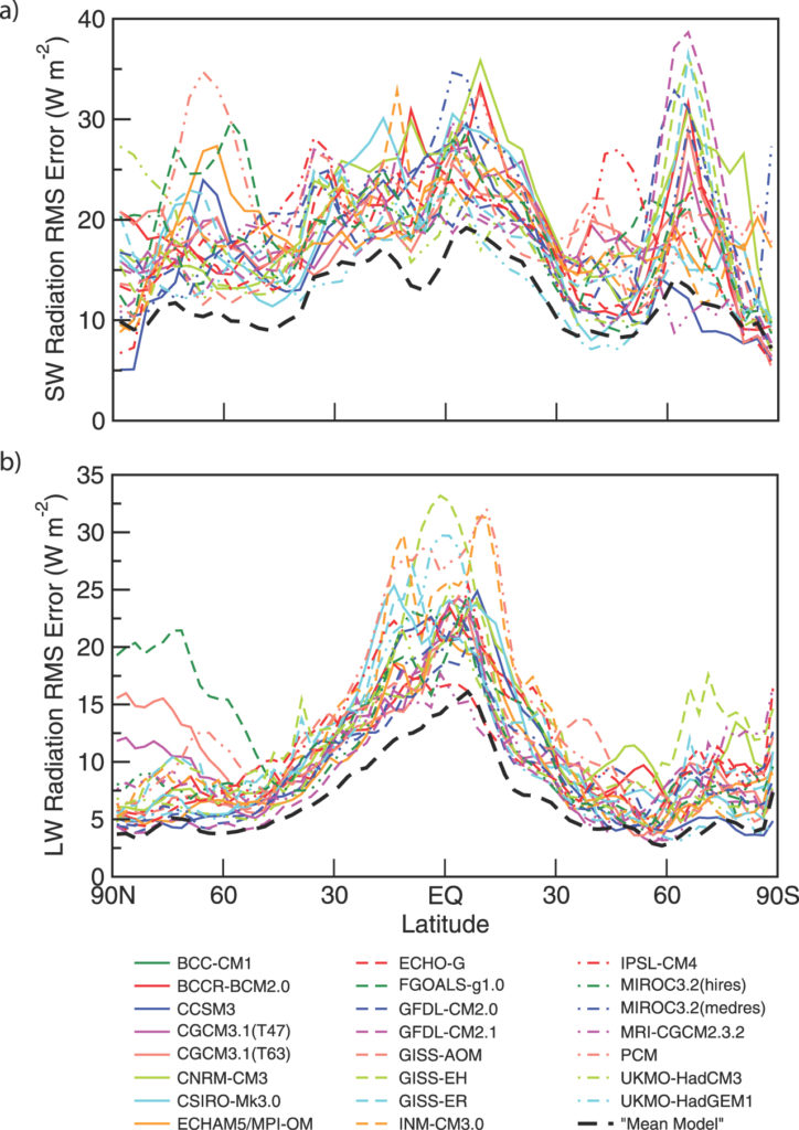
fig-8-04-724x1024

The accuracy of GCMs is reflected in the skill with which they simulate the TOA energy budget: the driver of climate. By construction, GCMs achieve global-mean energy balance. How faithfully the energy budget is represented locally, however, is another matter. The local energy budget forces regional climate, along with the gamut of weather phenomena that derive from it. This driver of regional conditions is determined internally – through the simulation of local heat flux, water vapor, and cloud. Symbolizing the local energy budget is net radiation (Fig. 1.34c), which represents the local imbalance between the SW and LW fluxes F0 and F ↑(0) in the TOA energy budget (8.82). Local values of those fluxes have been measured around the Earth by the three satellites of ERBE. The observed fluxes, averaged over time, have then been compared against coincident fluxes from climate simulations, likewise averaged. Figure 8.34 plots, for several GCMs, the rms error in simulated fluxes, which have been referenced against those observed by ERBE.

The significance of these discrepancies depends on application. Overall fluxes at TOA are controlled by water vapor and cloud (Fig. 1.32) – the major absorbers that account for the preponderance of downwelling LW flux to the Earth’s surface. Relative to those fluxes, the errors in Fig. 8.34 are manageable: Of order 10% for outgoing LW and 20% for reflected SW. Relative to minor absorbers, however, this is not the case. The entire contribution to the energy budget from CO2 is about 4 Wm−2. Errors in Fig. 8.34 are an order of magnitude greater. Consequently, the simulated change introduced by increased CO2 (2–4 Wm−2), even inclusive of feedback, is overshadowed by error in the simulated change of major absorbers.

Conclusion:

Pg. 262
Discrepancies between GCMs arise from inaccuracies in climate properties and from differences in how those properties are represented. Much of the discrepancy surrounds the representation of convection and its influence on water vapor and cloud, the absorbers that account for most of the downwelling LW flux to the Earth’s surface. The involvement of convection is strongly suggested by models of radiative-convective equilibrium. Those simulations are inherently sensitive to how convection and cloud are prescribed. Cloud is especially significant to radiative considerations because it sharply modifies the atmosphere’s scattering characteristics, which determine albedo, and its absorption characteristics, which determine optical depth.

Footnote:

Best wishes to Dr. Salby and much appreciation for telling it like it is. May you also nail your landing as did Fearless Felix.

h/t malagabay

Typical Arctic Melting June 15

Posted on June 15, 2016 by Ron Clutz

US Navy predicts summer ice free Arctic by 2016. Greenpeace icebreaking ship, Arctic Sunrise, among broken floes of Arctic sea ice, photographed from the air. This image was taken in the Fram Strait. Greenpeace doing their bit to create more open water.

In the chart below MASIE shows June Arctic ice extent has drawn nearer average and close to 2015 at this point in the year.

This year and last had the same average extents until May when a gap opened up associated with the Beaufort gyre high winds breaking up and moving ice to create 150k km2 open water in that sea. The difference in Beaufort Sea is now ~40k km2 between 2016 and 2015.

Looking into the details, some marginal seas are melting earlier than last year, while the central, enduring ice pack is relatively unaffected. In fact, a large difference between 2016 and 2015 comes from the losses from maximums in a single place: Sea of Okhotsk: To date 1275k km2 of ice lost this year vs. 740k km2 lost in 2015 in that sea at the same date.

Despite greater losses in Okhotsk, 2016 ice extent in June is nearly typical with slight differences across the regions. At the present pace of declining ice extents, 2016 is virtually tied with 2015 and running four days ahead of the ten-year average.

As the chart below shows, the seas down most this year include Beaufort, Barents, Greenland Sea, and Baffin Bay. Meanwhile higher extents are showing in Chukchi, Kara, Laptev and Hudson Bay, resulting in 2016 only slightly below 2015 overall. The Central Arctic Sea is slightly above 2015.

Ice Extents			Ice Extent
Region	2015166	2016166	km2 Diff.
(0) Northern_Hemisphere	10791329	10749626	-41703
(1) Beaufort_Sea	948114	906972	-41142
(2) Chukchi_Sea	747954	836166	88212
(3) East_Siberian_Sea	1084037	1084831	794
(4) Laptev_Sea	825271	890792	65522
(5) Kara_Sea	602369	674328	71959
(6) Barents_Sea	170125	76864	-93261
(7) Greenland_Sea	613376	532214	-81162
(8) Baffin_Bay_Gulf_of_St._Lawrence	776625	649408	-127218
(9) Canadian_Archipelago	790324	803589	13265
(10) Hudson_Bay	988976	1029192	40216
(11) Central_Arctic	3200053	3221196	21144
(12) Bering_Sea	3875	9080	5205
(13) Baltic_Sea	0	33	33
(14) Sea_of_Okhotsk	39088	33819	-5269

Comparing the Arctic ice extents with their maximums shows the melting is occurring mostly in the marginal seas, as expected in June.

2016166	NH Max Loss	% Loss Sea Max	% Total Loss
(0) Northern_Hemisphere	4327974	28.70%	100%
(1) Beaufort_Sea	163473	15.27%	3%
(2) Chukchi_Sea	129823	13.44%	3%
(3) East_Siberian_Sea	2289	0.21%	0%
(4) Laptev_Sea	7017	0.78%	0%
(5) Kara_Sea	260660	27.88%	6%
(6) Barents_Sea	522515	87.18%	11%
(7) Greenland_Sea	127498	19.33%	3%
(8) Baffin_Bay_Gulf_of_St._Lawrence	995175	60.51%	21%
(9) Canadian_Archipelago	49590	5.81%	1%
(10) Hudson_Bay	231679	18.37%	5%
(11) Central_Arctic	25514	0.79%	1%
(12) Bering_Sea	759152	98.82%	16%
(13) Baltic_Sea	97549	99.97%	2%
(14) Sea_of_Okhotsk	1274877	97.42%	27%

Note: Some seas are not at max on the NH max day. Thus, totals from adding losses will vary from NH daily total.

It is clear from the above that the bulk of ice losses are coming from Okhotsk, Barents and Bering Seas, along with Baffin Bay-St. Lawrence; all of them are marginal seas that will go down close to zero by September, and only Baffin has more than 12% of its ice left.

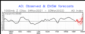
CPC shows the Arctic Oscillation waffling between positive and negative values, now forecasted to go positive. Generally, positive AO signifies lower pressures over Arctic ice, with more cloud, lower insolation and less melting. The outlook at this point is mixed.

September Minimum Outlook

Historically, where will ice be remaining when Arctic melting stops? Over the last 10 years, on average MASIE shows the annual minimum occurring about day 260. Of course in a given year, the daily minimum varies slightly a few days +/- from that.

For comparison, here are sea ice extents reported from 2007, 2012, 2014 and 2015 for day 260:

Arctic Regions	2007	2012	2014	2015
Central Arctic Sea	2.67	2.64	2.98	2.93
BCE	0.50	0.31	1.38	0.89
Greenland & CAA	0.56	0.41	0.55	0.46
Bits & Pieces	0.32	0.04	0.22	0.15
NH Total	4.05	3.40	5.13	4.44

Notes: Extents are in M km2. BCE region includes Beaufort, Chukchi and Eastern Siberian seas. Greenland Sea (not the ice sheet). Canadian Arctic Archipelago (CAA). Locations of the Bits and Pieces vary.

As the table shows, low NH minimums come mainly from ice losses in Central Arctic and BCE. The great 2012 cyclone hit both in order to set the recent record. The recovery since 2012 shows in 2014, with some dropoff last year, mostly in BCE.

Summary

We are well into the melt season, and the resulting minimum will depend upon the vagaries of weather between now and September. Early on, 2016 was slightly higher than 2015 in March, lower in May and now closing the gap. Note: 2016 melt season is starting without the Blob, with El Nino over, and a cold blob in the North Atlantic. The AO has been hovering around neutral, now possibly indicating cloud cover reducing the pace of melting.

Meanwhile we can watch and appreciate the beauty of the changing ice conditions.

Arctic Reflection: Clouds replace snow and ice as solar reflector NASA photo

Footnote: Regarding the colder than normal water in the North Atlantic

A 2016 article for EOS is entitled Atlantic Sea Ice Could Grow in the Next Decade

Changing ocean circulation in the North Atlantic could lead to winter sea ice coverage remaining steady and even growing in select regions.

The researchers analyzed simulations from the Community Earth System Model, modeling both atmosphere and ocean circulation. They found that decadal-scale trends in Arctic winter sea ice extent are largely explained by changes in ocean circulation rather than by large-scale external factors like anthropogenic warming.

From the Abstract of Yeager et al.

We present evidence that the extreme negative trends in Arctic winter sea-ice extent in the late 1990s were a predictable consequence of the preceding decade of persistent positive winter North Atlantic Oscillation (NAO) conditions and associated spin-up of the thermohaline circulation (THC). Initialized forecasts made with the Community Earth System Model decadal prediction system indicate that relatively low rates of North Atlantic Deep Water formation in recent years will result in a continuation of a THC spin-down that began more than a decade ago. Consequently, projected 10-year trends in winter Arctic winter sea-ice extent seem likely to be much more positive than has recently been observed, with the possibility of actual decadal growth in Atlantic sea-ice in the near future.

Circling the Climate Wagons

Posted on June 14, 2016 by Ron Clutz

What to make of this recent Report (here):

An Australian university recently censured marine scientist Paul Ridd for “failing to act in a collegial way and in the academic spirit of the institution,” because he questioned popular claims among environmentalists about coral reefs and global warming.

To understand what is going on, some background in organizational sociology is helpful.

In past decades, researchers looking into organizational behavior concluded that the internal discipline inside the organization had to be stronger than the threats or enticements outside. Thus, an army has high regimentation and command drilling in order that soldiers follow orders and perform in the face of armed enemies trying to kill them. Police units operate in hostile environments and rely on similar training and disciplines.

Slightly different examples include missionaries seeking to convert heathens, without themselves losing their beliefs, religous practices or ethics when surrounded by people of another culture.

When it comes to corporations, most of them have sales departments who have a special camaraderie and rituals that keep them pitching skeptical customers in the face of rejection and losing trades to competitors.

All this is context for recognizing that many scientists in the present research funding market operate as salesmen in order to protect and enhance their revenue streams. If they are prone to exaggerated claims, that goes with the role and territory. And if they are called to account for not having the back of fellow salesmen, that is also to be expected.

The behavior of climate scientists at James Cook University is a case of sales managers attacking the credentials of someone undermining their claims and threatening to dispel the fears upon which government funding is based.

Sadly, this is further evidence of the degradation of climate science, which has been thoroughly vetted by Richard Lindzen: Climate Science Was Broken

Cooling Outlook

Posted on June 13, 2016 by Ron Clutz

The RAPID moorings being deployed in North Atlantic. Credit: National Oceanography Centre

In the comments on a previous post (here) ren points to the declining NAO, with the implication that a cooling phase is underway in the North Atlantic SSTs. The cold blob in the North Atlantic was subject of a post here and elsewhere, and Paul Homewood posts today (here) on the increasing cold water, not only surface but coming from below.

Dr. Gerard McCarthy is a lead researcher on the RAPID array project measuring the AMO heat transport and provides a good context on their observations and the implications for the climate cooling in coming decades.

Our results show that ocean circulation responds to the first mode of Atlantic atmospheric forcing, the North Atlantic Oscillation, through circulation changes between the subtropical and subpolar gyres – the intergyre region. This a major influence on the wind patterns and the heat transferred between the atmosphere and ocean.

The observations that we do have of the Atlantic overturning circulation over the past ten years show that it is declining. As a result, we expect the AMO is moving to a negative (colder surface waters) phase. This is consistent with observations of temperature in the North Atlantic.

Summary:

The Atlantic Ocean’s surface temperature swings between warm and cold phases every few decades. Like its higher-frequency Pacific relative El Nino, this so-called “Atlantic Multidecadal Oscillation” can alter weather patterns throughout the world. The warmer spell we’ve seen since the late 1990s has generally meant warmer conditions in Ireland and Britain, more North Atlantic hurricanes, and worse droughts in the US Midwest.

However a colder phase in the Atlantic could bring drought and consequent famine to the developing countries of Africa’s Sahel region. In the UK it would offer a brief respite from the rise of global temperatures, while less rainfall would mean more frequent summer barbeques. A cold Atlantic also means fewer hurricanes hitting the southern US.

https://www.weforum.org/agenda/2015/06/how-the-atlantics-cool-phase-will-change-the-worlds-weather/

Implications for Arctic Ice

A 2016 article for EOS is entitled Atlantic Sea Ice Could Grow in the Next Decade

Changing ocean circulation in the North Atlantic could lead to winter sea ice coverage remaining steady and even growing in select regions.

From the Abstract of Yeager et al.

Historic Climate Change

Posted on June 12, 2016 by Ron Clutz

Orbital Climate Factors: E for eccentricity, T for tilt, and P for precession

My recent post The Coming Climate included a description of the orbital factors inducing natural cycles of warming and cooling far larger than any possible effect from CO2.

Yesterday commenter Alberto Zaragoza Comendador took this further into a discussion of the uncertainties in paleoclimatology. He started by referring to a paper by Lindzen, which focused on only one of these dynamics: fluxes of equator-to-pole heat transport.

Lindzen et al. 1993 concluded:
The present note shows the importance of aspects of the forcing which lead to changes in meridional (i.e., tropics to higher latitudes) heat fluxes. These aspects are seasonal, and involve the distribution of heating; they do not necessarily involve changes in globally and/or annually averaged insolation. Thus, simple, commonly used notions of climate sensitivity as employed in Houghton et al. (1990) are not relevant. Indeed, the present mechanism can readily produce major changes in climate (including, as a by product, changes in the globally averaged temperature) in systems which are profoundly insensitive to a doubling of CO2. To assume (as was done in Hoffert and Covey 1992, for example) that major climate changes necessarily require high sensitivity to such changes in gross averaged forcing is clearly inappropriate.

The full text of comment by Comendador is below from Climate Etc. (here)

Alberto Zaragoza Comendador | June 11, 2016 at 3:19 pm |

Somebody mentioned Milankovitch which reminded me of other thing.

http://www-eaps.mit.edu/faculty/lindzen/171nocephf.pdf (Lindzen et al 1993)

Check out the last paragraph. It explains why every paleo estimate of sensitivity is hopeless: even if you knew the temperatures, which you don’t really but even if you did, you’d have no idea what caused them. Lindzen uses the example of equator-to-pole heat transport but there are many more things that can cause climate to change, and we mostly know nothing about how they affected climate in the past.

We have records of methane and CO2, but we don’t have records of cloud albedo, ozone, water vapor, vegetation… someone might quibble that we do have some records of vegetation and dust for example, but unlike CH4 and CO2 you cannot assume these dust or vegetation ‘levels’ applied globally.

(Hell, until recently the greening trend of the last half-century was in dispute, even though we can look at the world’s plants and trees with seven billion pairs of eyes plus a few billion cameras, including some mounted on satellites. To assume we can now estimate greening or browning trends from twenty thousand years ago is preposterous.)

And we have estimates of how much area was covered in ice, but we have no idea how much dust that ice was covered with, or if the radiative forcing one could expect from the ice was really ‘apples to apples’ (i.e. of the same efficacy) as that of CO2. Now we know that as sea ice recedes the Arctic gets cloudier so the overall effect is about 1/3 of what you would expect simply looking at the decline in ice; we have no idea if the same thing would happen upon the disappearance of an ice sheet because we have never observed such a thing. Until recently we thought Greenland was reflecting less sunlight because it was getting dustier; it then turned out that, rather, the satellites’ sensors were getting degraded.

We still have little idea how aerosols affect climate… yet some guys are trying to model the aerosols of the past. And they’re not even the same kind (today the main agent is sulphuric acid, before dust).

(It’s funny that the ‘forcing efficacy’ issue has been raised about instrumental studies, and not about paleo papers that would be devastated if efficacy really changed much between forcing agents. For example, only about 20% of the forcing in LGM reconstructions is CO2).

You cannot simply assume that whatever change in GHG concentration (or other ‘forcings’) took place at the time of these temperature changes was responsible for said changes. In fact, by excluding other factors (which you know nothing about) you will systematically overestimate sensitivity. That’s why paleo sensitivity disagrees with both energy budget and inter-annual (ERBE/CERES) estimates. It also explains in part why the range of sensitivity in paleo is so wide.

Admittedly this is also a strike against sensitivity estimates using the instrumental record, but less so – because we have observations that allow us to rule out a good many ‘natural’ causes of climate change. We know that in the last 150 years the AMOC hasn’t shut down and there hasn’t been a massive change in equator-to-pole heat transfer. We know that since 1980 the amount of cloud cover has remained more or less the same, within a 5% band; the warming trend since then would be very difficult to explain from changes in cloud cover alone. And so on.

Whenever one mentions natural climate change the response from a certain side is something like ‘the ocean cannot create heat’ or ‘the clouds cannot change by themselves’. While technically true these statements are meaningless and reveal at best ignorance and at worst deception. All climate changes will involve a radiative change at some point, but said radiative change (forcing, feedback, whatever you call it) does NOT have to originate from a radiative source. It can all start with a change in air currents, or ocean currents, or tree cover, or sea ice, or methane emissions from bacteria, or…

Asking ‘yeah but what caused the clouds to change?’ is like asking why are there planets.

The best example of non-radiative climate change is in fact Milankovitch cycles, which affect not the amount but the distribution of sunlight (well eccentricity changes the amount of sunlight, but precession and tilt don’t). Technically speaking, the forcing is zero; paleo estimates consider GHGs, ice sheets and vegetation/dust forcings but if one is strict they should be considered feedbacks. Sensitivity, calculated the way it’s done for observational estimates, would be infinite.

You can also see how simply switching one of these radiative ‘things’ from forcing to feedback, or viceversa, can allow a researcher to arrive at a radically different sensitivity number. It’s all meaningless.

The one advantage of the paleo method is that since there is enough time for the ocean to reach equilibrium you avoid that source of uncertainty. But that also means you cannot use it to estimate TCR.

Anyway, as time goes on the estimates of aerosol forcing and heat uptake will get better and better. The instrumental studies will arrive at a number, if not for what sensitivity ‘is’, at least for what it has been for the last 150 years. The paleos will never arrive at anything.

Conclusion:

Thanks Alberto for that summation. It deserves wide appreciation

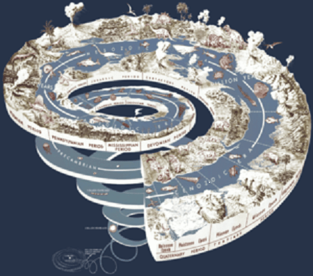
Geological Time Spirial

Wave Drowns CO2 Warming

Posted on June 9, 2016 by Ron Clutz

Update May 13 below

This post presents key findings from the recently published paper:
Anthropogenic CO2 warming challenged by 60-year cycle (here) by
François Gervais
Department of Physics, Faculty of Sciences & Techniques, François Rabelais University, Parc de Grandmont, 37200 Tours, France

In the synopsis below, Gervais puts his study in context, followed by his conclusions.

The Global Warming Debate Rages

The impact on climate of the CO2 emitted by burning of fossil fuels is a long-standing debate illustrated by 1637 papers found in the Web of Science by crossing the keywords

“anthropogenic” AND “greenhouse OR CO2” AND “warming”

This is to be compared to more than 1350 peer-reviewed papers which express reservations about dangerous anthropogenic CO2 warming and/or insist on the natural variability of climate.

Signatures of 60-year Climate Wave

Time series of sea-level rise are fitted by a sinusoid of period ~ 60 years, confirming the cycle reported for the global mean temperature of the earth. This cycle appears in phase with the Atlantic Multidecadal Oscillation (AMO). The last maximum of the sinusoid coincides with the temperature plateau observed since the end of the 20th century. A 60-year climate cycle is confirmed in sea-level rise and global sea ice area, as well as in measured temperature series.

Onset of the Declining Phase

The four following indicators sign for the onset of the declining phase of the 60-year cycle.

The recent change of sign of global sea ice area anomaly which
reveals an excess in Fig. 3, a sensitive indicator of climate, is unexpected
from model projections (AR5, 2013).
The AMO index indicates the onset of a declining phase.
A negative temperature slope is measured from 2002 to 2015 independently by different satellites in the low troposphere by Remote Sensing System (RSS, 2015) and by UAH (Spencer et al., 2015) as shown in Fig. 4. The plot is voluntarily restricted to 13 years, viz. less than 1/4 of the 60 year-cycle, to evaluate the sign of the tangent to the sinusoid.
A deceleration of the sea-level rise measured by satellite altimetry is also found since 2002 (Chen et al., 2014; Cazenave et al.,2014).

Rising Temperatures cause rising CO2

The correlation of yearly CO2 increase, therefore, appears not with MEI or SOI but with global mean temperature to which El Niño and La Niña contribute. This temperature/CO2 correlation may be tentatively explained, at least partly, by the solubility of CO2 into water which decreases with temperature, consistent with sea pH maps (Byrne et al., 2010). Warm temperature fluctuations favor CO2 release from the oceans which contain 60 times more CO2 than the atmosphere (AR5, 2013), whereas cooler fluctuations favor its oceanic Capture.

Summary: 60-year Wave Rules

Dangerous anthropogenic warming is questioned (i) upon recognition of the large amplitude of the natural 60–year cyclic component and (ii) upon revision downwards of the transient climate response consistent with latest tendencies shown in Fig. 1, here found to be at most 0.6 °C once the natural component has been removed, consistent with latest infrared studies (Harde, 2014). Anthropogenic warming well below the potentially dangerous range were reported in older and recent studies. On inspection of a risk of anthropogenic warming thus toned down, a change of paradigm which highlights a benefit for mankind related to the increase of plant feeding and crops yields by enhanced CO2 photosynthesis is suggested.

The whole paper is well worth the read, and is chock full of links to sources and references supporting his analysis.

Here is a recent Youtube video of Francois Gervais presenting his findings (with English translation)

Update May 13

In the comments below ren points to the declining NAO, with the implication that a cooling phase is underway in the North Atlantic SSTs. The cold blob in the North Atlantic was subject of a post here and elsewhere, and Paul Homewood posts today on the increasing cold water, not only surface but coming from below.

The observations that we do have of the Atlantic overturning circulation over the past ten years show that it is declining. As a result, we expect the AMO is moving to a negative (colder surfer waters) phase. This is consistent with observations of temperature in the North Atlantic.