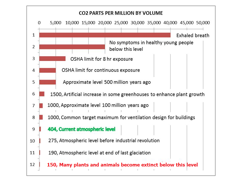
From “Show me the money” to “Show me your work”

Much of what is wrong with climate science started when they switched from real world observations to building and playing with computer toy models of the world. Much of the research money has gone into climate modelling, which has yet to show skill in predicting changes in weather patterns on any time scale beyond a few weeks. The models themselves are confused by their makers with the real world, and they even refer to computer runs as “experiments.”

Almost 2 years ago I became aware of Dr. Arnd Bernaerts’ insightful phrase, “Climate is the continuation of the ocean by other means.” From oceanographic observations, he has long been persuaded the climate changes because of ocean oscillations, and I learned a lot from him while writing a number of posts here collected under the category Oceans Make Climate.

Arnd is also persuaded that humans are impacting on the oceans, and thereby upon the climate, but by obvious maritime activities and not by CO2 emissions. For his impertinence, he was “disappeared” from Wikipedia by the zealots there who purge that website from sources and information skeptical of global warming dogma.

As happened in Soviet history, climate revisionists are rewriting history.

As happened in Soviet history, climate revisionists are rewriting history.

Dr. Bernaerts continues to write on climate and ocean matters, most recently at his website: Oceans Govern Climate

Ironically, alarmists are crowing right now about Arctic ice extent being a little lower this year, while not mentioning most of the deficit is due to Barents Sea, and secondly to less ice in Bering Sea. Both of those places are subject to extensive maritime activity–shipping, fishing, oil and mineral exploration and extraction, and icebreaking to support year-round operations. Bernaerts explains: Man-Made Ocean Warming? Yes, but it’s not CO2.

Activist scientists, fixated on models and global warming, are indifferent to the correlation between WWI Atlantic naval warfare and unprecedented warming at Spitzbergen (Svalbard). Only an evidence-based scientist like Bernaerts is paying attention, as I have reported previously (here).

Another example of how science is perverted to support a political climate agenda was provided by commenter crypto666 referring to Matt Lachniet’s research into the former ocean basin in Nevada. By happenstance, Bernaerts had visited the Great basin last September (If you’re devoted to the oceans, I guess you are interested even in prehistoric, dried-out basins.)

Lachniet is properly circumspect in his writing and presentations, noting his findings pertain to a particular location, and suggesting several possible explanations for anomalous warming starting 1600 years ago. Yet his research was twisted into a climate change warning by journalists writing in the Las Vegas Sun (here).

As crypto points out, this is not what Lachniet himself has said. He is as clear as anyone that warming starting in the Fifth century did not come from people driving SUVs, so some natural oscillations must be in play. (California terminology: SUV=Axle of Evil).

Summary

My hope for 2017 is to begin seeing a regime shift in climate science from “Show me the money” to “Here are my data and work, Let the chips fall where they may.” Natural scientists have always owned a sense of awe alongside their curiosity, appreciating the enormity of the world they seek to understand. Dr. Bernaerts is right to remind us that even with modern technologies, our hard-won observational data is a minuscule sampling of oceanic and atmospheric activities. Any conclusions to be drawn should be put forward with humility. The dogmatic positions of climate alarmists are a disgrace to the profession.

Footnote: Below are reprinted relevant comments from Bernaerts and crypto.

Arnd Bernaerts said:

Hi Ron, having been to the Great Basin/NV recently, I couldn’t resist asking: what have 3,500 Argo floats and other ocean sensors (image caption) and the Matt Lachniet „nevada-caves-climate-change” (link in one of your comments) in common?
In – MHO – a lot, as they are both of little help to understand how to prevent anthropogenic climate change sufficiently. Recalling my visit of the Lehman caves a few days earlier or later (on 9th September) as Matt Lachniet, the cave formation was impressive, but hardly of any use for current concern.

3,500 Argo floats are certainly a more promising approach. But if one considers the dimension (& temperatures) in which they operate; nicely outlined recently at https://wattsupwiththat.com/2016/12/26/warming-by-less-upwelling-of-cold-ocean-water/, it is like reading from stalactite about AGW matters.

The use of Argo floats is an achievement, but by far too small. Observations below the sea surface would require a number of several hundred thousand, if not millions of devices (and the capability to process the data sufficiently). After all we need to understand the role of the oceans, and whether they bring a severe cooling, which is possible at any time.

Ron, to you, your family and everybody calling at this site:
HAPPY NEW YEAR

crypto666 said:

Thanks for pointing that out Ron. All I can say is unbelievable.

“Lachniet’s Great Basin research suggests that, based on the Earth’s orbit, the region should not be in a dry period. But it is. In any scenario, human-caused climate change, amplified over the next few centuries by natural warming, could be troublesome for a place that’s already notoriously dry and hot.”

The first thing I will point out however, is that those are not his words. Those are the words of the article writer. It is also either an outright lie, or a mistake. Another writer from the UNLV paper tried saying that Matt’s research suggests humans started changing the climate 1,600ybp, which again is not the case.

I know Matt, and he delivered his 2014 study to my colleagues and myself personally. After we talked for a bit, and surprised him by identifying that change in trend before he did in his work, which he identified as being 1,600 ybp, I asked him what his thoughts were on co2. What I vividly remember is Matt pointing to his chart and stating that he doesn’t think anyone will be able to identify co2’s contribution to climate change until we reached the point of his finger, which is where we should start the long road back to glaciation. It may have 2ky or maybe it was 55ky, at any rate what he says in person isn’t exactly what you get from news articles and twitter feeds.
I will also point out this:

A Speleothem Record of Great Basin Paleoclimate
January 2016
DOI: 10.1016/B978-0-444-63590-7.00020-2
In book: Lake Bonneville – A Scientific Update, pp.551-569

https://www.researchgate.net/publica…n_Paleoclimate

“The lag behind NHSI of d18O variations suggests that the forcing is indirect. Several possible forcings are associated with the Great Basin d18O variations. First, it is clear that CO2 concentrations increase abruptly around the MIS 2/1 and MIS 6/5d transitions, which may explain some of the warming over Terminations I and II. However, Nevada d18O values drop steadily throughout the Holocene, whereas CO2 remains high and even increases slightly over the last 8000 years (Ruddiman, 2003). Similarly, the strongly low d18O values during MIS 5d and MIS 7 happen during intervals with intermediate to high CO2 values.

Thus, the CO2 changes may amplify a warming already in progress around ice volume terminations but are unlikely to be the source of the climate change, because they are decoupled during prominent intervals such as MIS 1 and 5d. A related hypothesis suffers from similar problems: the extent of the Laurentide Ice Sheet (LIS). The LIS retreated over the MIS 2/1 and MIS 6/5 transitions when temperatures in the Great Basin warmed (as inferred by increasing d18O values). However, decreasing d18O values from 8 ka to modern happened in the absence of any ice-sheet regrowth, and the prominent MIS 5d and MIS 7 minima also happened when ice sheets were small. Thus ice-sheet extent cannot be the primary driver of Great Basin d18O variations. The clear conclusion is that neither CO2 nor ice-sheet extent were the sole or dominant controls on Great Basin paleoclimate over orbital timescales.”

That conclusion doesn’t strike me as coming from someone who believes co2 controls climate.  There is a big leap from believing that co2 could cause increased heating of the atmosphere, and thinking co2 controls climate and/or we can control climate with co2.

I have actually had people try to use Mr. Lachniet’s twitter account in an attempt to change the conclusion of his studies. Which is always entertaining.

Pesky Australian Alarmists

Those pesky Australian alarmists sure do like to exaggerate. First they sold everyone that the “Science is Settled. Fossil fuels are warming the planet dangerously.” The government said: “We accept your report, thank you for your service,” and followed up with a plan to downsize the climate research unit (CSIRO).

Then came their loud public outcry: “You can’t do that. There is so much we don’t know and have to study. We need those jobs.”  So the government walked back that plan.

Now Australian scientists figure to build on their success by writing an open letter to the Prime Minister urging action to “fight climate change.”  And, no surprise, Exhibit A is the threat to the Great Barrier Reef. Trouble is, once again they are exaggerating and hoping no one will notice. The bluff is being called by people who visit and dive the reefs every day.

April 2016 Observations

New research found about 68 per cent of reefs from Cairns to Lizard Island had varying levels of coral bleaching, but most of it likened to sunburn on a human body where the coral glows pink before fully recovering.

Latest findings by the Reef and Rainforest Research Centre give hope about the resilience of the living wonder after scientists this week revealed 93 per cent of the 2300km-long reef system was in the grip of a mass bleaching event.

Great Barrier Reef as seen by Activists. (Later Greenpeace admitted the image is a storm-damaged reef in the Philippines).

“It’s the Great White Lie,” said Col McKenzie, chief executive of the Association of Marine Park Tourism Operators. “It’s not dead, white and dying. It’s under stress but it will bounce back.’’

Coral bleaching is linked to high water temperatures of the latest El Niño weather system, where stressed coral polyps eject their photosynthetic zooxanthellae and, in extreme cases, the living colony will appear totally white. Skeletons are covered in algae.

The RRRC report found on the 126 key tourists sites there was, on average, 35 per cent coral cover – about one-third unbleached – and, on average, only 2.5 per cent of the coral had died because of bleaching.  “We think there is a much lower level of severely bleached corals. To say 80 per cent of the reef will die is catastrophising the situation,’’ RRRC director Sheriden Morris said. Source: Great Barrier Reef: Signs of recovery despite major coral bleaching, The Courier-Mail, Brisbane

That was in April.  In June Alarmists doubled down on their deceit by excommunicating one of their own for calling them out on their exaggerations (here):

An Australian university recently censured marine scientist Paul Ridd for “failing to act in a collegial way and in the academic spirit of the institution,” because he questioned popular claims among environmentalists about coral reefs and global warming.  Background post Circling the Climate Wagons

Great Barrier Reef photographed by Ronald Hanko June 16, 2016.

Updated Observations of Great Barrier Reef

In April 2016 the reef bleaching from El Nino was at its peak and occasioned widespread alarms. Now this week we have an observational update

Great Barrier Reef tourist operators found less than 5 percent of the natural wonder has died off from “bleaching,” despite claims from scientists that most of the reef had been killed off by the effects of global warming.  “Scientists had written off that entire northern section as a complete white-out,’’ Chris Eade, owner of the diving boat Spirit Of Freedom, told The Courier-Mail in an interview.

“We expected the worst,” Eade said. “But it is in tremendous condition, most of it is pristine, the rest is in full recovery. It shows the resilience of the reef.”

“It wasn’t until we got underwater that we could get a true picture of what percentage of reef was bleached,’’ Craig Stephens, who manages Mike Ball Dive Expeditions, told The Courier-Mail.

Stephens has surveyed the reef and compared his findings to a similar survey he did 20 years ago. He found almost no change between what he saw back then and today.

“Coral mortality in the outer shelf reefs north of Lizard Island was between one and five per cent,” according to findings exclusively obtained by The Courier-Mail. This stands in sharp contrast to reports from April of 50 percent bleaching in the northern section of the reef.

“The discrepancy is phenomenal. It is so wrong. Everywhere we have been we have found healthy reefs,” Stephens said.

Conclusion

Down under the alarmist icon is the Great Barrier Reef. In the North of course, it is the Arctic Polar Bear.

Update Aug. 26 Yes PM Pokes Fun at Climatism

Update May 12, 2017

This video seems to work for everyone:

Update Aug. 26, 2016 Below

In Feb. 2016 I posted this:

A humorous look at why the global warming campaign and the triumphal Paris COP make sense.

Yes Minister explains it all in an episode from 2013.

h/t to Peter S.

This is an all-too-realistic portrayal of political climatism today.

Update Aug. 26, 2016

Yesterday I realized that BBC had blocked the viewing of the video.  So I sought and found the subtitles for Yes Prime Minister 2013, Episode 6, “A Tsar is Born”.  That final episode for the series began with the dialogue in yesterday’s post Climate Alarms LOL.

Today I provide the dialogue that formed the episode conclusion, and which was the content of the blocked video.

The Characters are:

Sir Humphrey Appleby
Cabinet Secretary

Jim Hacker
Prime Minister

Claire Sutton
Special Policy Adviser

Bernard Woolley
Principal Private Secretary to the Prime Minister

(Dialogue beginning at 20:16 of “A Tsar is Born”)

Humphrey I have returned with the answer to all your problems.
Global warming.

Jim I thought you were against it?

Humphrey Everybody’s against it, Prime Minister.
I suddenly realised that is the beauty of it.
We can get a unanimous agreement with all of our European partners
to do something about it.

Jim But how can we do something about
something that isn’t happening?

Humphrey It’s much easier to solve an
imaginary problem than a real one.

Jim You believe it’s real?

Humphrey Do you? I don’t know.

Jim Neither do I. Haven’t got the faintest idea!

Humphrey But it doesn’t matter what we think.
If everyone else thinks it’s real, they’ll all want to stop it.
So long as it doesn’t cost too much.
So the question now is, what are we going to do about it?

Jim But if it isn’t happening, what can we do about it?

Humphrey Oh, there’s so much we can do, Prime Minister.
We can impose taxes, we can stiffen European rules about
carbon emissions, rubbish disposal.

We can make massive investments in wind turbines.
We can, in fact, Prime Minister, under your leadership, agree to save the world.

Jim Well, I like that!
But Russia, India, China, Brazil, they’ll never cooperate.

Humphrey They don’t have to. We simply ask them to review their emissions policy.

Jim And will they?

Humphrey Yes. And then they’ll decide not to change it.
So we’ll set up a series of international conferences.
Meanwhile, Prime Minister, you can talk about the future of the planet.

Jim Yes.

Humphrey You can look statesmanlike.
And it’ll be 50 years before anybody can possibly prove you’re wrong.
And you can explain away anything you said before by saying the computer models were flawed.

Jim The voters will love me!

Humphrey You’ll have more government expenditure.

Jim Yes. How will we pay for it? We’re broke.

Humphrey We impose a special global warming tax on fuel now,
but we phase in the actual expenditure gradually. Say, over 50 years?
That will get us out of the hole for now.

Bernard The Germans will be pleased.
They have a big green movement.

Claire And we can even get the progs on board!

Bernard As long as they get more benefits than everyone else.

Jim My broadcast is on Sunday morning.

Humphrey You have a day to get the conference to agree.

Jim That’s not a problem.
The delegates will be desperate for something to announce
when they get home.
There is one problem.
Nothing will have actually been achieved.

Humphrey It will sound as though it has.
So people will think it has.
That’s all that matters!

(Later following the BBC interview, beginning 27:34)

Bernard Oh, magnificent, Prime Minister!

Humphrey I think you got away with it, Jim,
but the cabinet will have been pretty surprised.
We’ll have to square them fast.

Jim Bubbles!

Humphrey We’re not there yet.
After that interview, you’ll need to announce some pretty impressive action.

Jim An initiative.

Humphrey Yes.

Claire A working party?

Humphrey Bit lightweight.

Bernard A taskforce?

Humphrey Not sure.

Jim Do we have enough in the kitty?

Claire It could be one of those initiatives that you announce
but never actually spend the money.

Jim Great. Like the one on child poverty.

Bernard Maybe it should be a government committee?

Jim Well what about a Royal Commission?

Humphrey Yes!
It won’t report for three years, and if we put the right people
on it, they’ll never agree about anything important.

Jim Right! A Royal Commission!
No, wait a minute, that makes it sound as if we think
it’s important but not urgent.

Claire Well, what about a Global Warming Tsar?

Jim Fine! Would that do it?

Humphrey No, I think it might need a bit more than that, Prime Minister.
It’ll mean announcing quite a big unit, and an impressive salary for that Tsar,
to show how much importance you place upon him.

Jim No problem. Who would it be?

Humphrey Ah, well, it can’t be a political figure.
That would be too divisive.
It has to be somebody impartial.

Jim You mean a judge?

Humphrey No, somebody from the real world.
Somebody who knows how to operate the levers of power,
to engage the gears of the Whitehall machine,
to drive the engine of government.

Jim That’s quite a tall order.
Anybody got any ideas?

Humphrey… Could you?

Bernard Oh!

Humphrey Yes, Prime Minister.

The End.

Footnote

CO2 hysteria is addictive. Here’s what it does to your brain:

Just say No!


The Coming Climate

Update July 4 below

When you see a graph like that below, it is obvious that an unusually strong El Nino just happened in our climate system. It resulted in higher global temperatures the last two years and so far in 2016. But that event is over now, and naturally we wonder what to expect in the months and years ahead.

cdas_v2_hemisphere_2016june2
For example some comments from a recent thread at WUWT (here) were intriguing:

It will be interesting to see what comes next. The major difference between the 1998 el nino and this one is that in 1998 the sun was increasing in solar activity, while this one solar activity is decreasing. (rishrac)

Nino3,4 and UAH LT dC Anomalies, and UAH LT Scaled *3 and Lagged 4 Months h/t Allan MacRae

And richard takes the long view of the situation:

While we all stare at the short-term ups and downs of the global temperatures, pay a little thought to the fact that the Earth’s orbit around the Sun causes snow in the winter and warmth during the summer, so it may be important?

Perihelion presently occurs around January 3, (Northern hemisphere winter, Southern summer) while aphelion is around July 4. Therefore, the southern hemisphere receives more solar radiation and is therefore warmer in summer and colder in winter (aphelion). The Northern hemisphere has cooler summers and milder winter (solar radiation-wise).

Also the northern hemispheres autumn and winter are slightly shorter than spring and summer, because the Earth is moving faster around the Sun in winter slower in summer.

This alone could account for “Global Warming” attributed to CO2, (which no doubt plays some part in it).

Over the next 10,000 years, northern hemisphere winters will become gradually longer and summers will become shorter, due to the change in the Earth’s Orbital Eccentricity.

Couple this with changes in the Earth’s tilt, which varies from 22.1 degrees to 24.5 degrees, (currently at 23.4 degrees). More tilt means more solar radiation gets to the poles (global warming) and less tilt means less radiation gets to the poles (global cooling). The last maximum tilt occurred in 8700 BC (Holocene maximum) and the next minimum tilt will happen in 11,800 AD (the advance of the ice sheets), precisely at the time of longer northern winters and shorter summers.

Orbital Climate Factors: E for eccentricity, T for tilt, and P for precession

Predicting the Future is Tough

Chiefio (E.M. Smith) has a good post (here) reminding us that statistical projections do not help us much in this case. Temperature series produced by our climate system have special qualities. The patterns are auto-correlated, meaning that tomorrow’s weather will be similar to today’s; the occurrence is not totally independent, like the flip of coin. IOW there is momentum in the climate characteristics, which can and do fluctuate over seasons, decades, centuries and more. Our attempts to use linear regressions to forecast are thwarted by temperature time series that do not follow a normal gaussian distribution, and are semi-chaotic and non-stationary.

Four Possibilities Forward From Today

From past experience, the next few years could logically follow one of four temperature scenarios:
1. The Plateau since 1998 continues.
2. The Warming prior to 1998 resumes.
3. A new Plateau begins with 2016 at a higher (step up) level.
4. A Cooling begins comparable to the years after 1940.

All of these have analogues in our recent climate observations. If this now finished El Nino triggers a regime change comparable to the 1998 event, then a step-up plateau can result. If warmists are right, and there is a release of pent-up heat in the system, then a warming trend would resume.

If this El Nino is not strong enough to shift the regime, then the Plateau could continue at the same level. Finally, it could be that several factors align to reverse the warming since the 1970’s, and bring a return to cooler 1950’s weather.

Those who see a quasi-60 year cycle in weather patterns note that it is about time for the PDO in the Pacific and the AMO in the Atlantic to be in cooler phases, along with a quiet sun, which went spotless last week. There are also those attending to orbital climate patterns, which gave us the Modern Warming Period and will eventually take it away.


Changes in climate due to earth’s orbit around the sun

Update July 4

In the thread below is a chart from J Martin displaying the effects of the changing tilt of earth’s axis.  As shown, the long term pattern is toward cooling.

In addition, ren provides interesting links to studies showing SA (Sunspot numbers) correlating to Middle Ages Warm period and LIA, and a 2012 study forecasting the next 2 cycles.

Figure 1. Bottom plot: the summary component of the two PCs (solid curve) and the decaying component (dashed curves) for the “historical” data (cycles 21–23) and predicted data (cycles 24–26). The cycle lengths (about 11 yr) are marked with different colors.
shepherd etalfig1

Again, to the extent that SSNs are a proxy for changes in heat content within the earth’s climate system, the graph is also indicating future cooling.

For quantification of climate effects from Solar Activity, see:
Quantifying Natural Climate Change

Climate Partly Cloudy

Dr. Curry has a new very informative post (here) on clouds and climate, including links to several studies recently announced from CERN and others. It reminded me of Joni Mitchell’s song Both Sides Now:

Bows and flows of angel hair
And ice cream castles in the air
And feather canyons everywhere
I’ve looked at clouds that way
But now they only block the sun
They rain and snow on everyone
So many things I would have done
But clouds got in my way

I’ve looked at clouds from both sides now
From up and down and still somehow
It’s clouds’ illusions I recall
I really don’t know clouds at all
– Joni Mitchell – Both Sides Now Lyrics

The above chorus could serve as an anthem for climate modelers. Clouds are arguably the least understood and most unpredictable of factors in climate change. We are getting much better at the weather connection between storms and cloud formation. But the long-term effects of clouds and cloudiness are still uncertain. Dr. Curry helpfully separates the cloud problem into two issues: cloud microphysics and cloud dynamics. She observes that the latter is much more difficult and also has much more impact on climate.

Some things are known and described in textbooks of Atmospheric Physics. In introducing Chapter 9: Aerosols and Clouds in his updated volume, Murray Salby (here) suggests the complexities involved:

Radiative transfer is modified importantly by cloud. Owing to its high reflectivity in the visible, cloud shields the Earth-atmosphere system from solar radiation. It therefore introduces cooling in the SW energy budget of the Earth’s surface, offsetting the greenhouse effect. Conversely, the strong absorptivity in the IR of water and ice sharply increases the optical depth of the atmosphere. Cloud thus introduces warming in the LW energy budget of the Earth’s surface, reinforcing the greenhouse effect. We develop cloud processes from a morphological description of atmospheric aerosol, without which cloud would not form. The microphysics controlling cloud formation is then examined. Macrophysical properties of cloud are developed in terms of environmental conditions that control the formation of particular cloud types. These fundamental considerations culminate in descriptions of radiative and chemical processes that involve cloud.

Cloud Formation

The microphysics is mostly related to how clouds form, and the role of aerosols. Even though clouds can form simply from enough water vapor, in practice the required conditions for such “homogenous” formation are higher than those needed for “heterogenous” formation from ever-present aerosols, termed CCN. From Salby (pg. 272):

The simplest means of forming cloud is through homogeneous nucleation, wherein pure vapor condenses to form droplets. . . Yet, the formation of most cloud cannot be explained by homogeneous nucleation. Instead, cloud droplets form through heterogeneous nucleation, wherein water vapor condenses onto existing particles of atmospheric aerosol. Termed cloud condensation nuclei (CCN), such particles support condensation at supersaturations well below those required for homogeneous nucleation.

Cloudiness Impact on Radiative Balance

The extent of cloudiness varies a lot, as shown by measures of OLR (Outgoing Longwave Radiation) by satellites above TOA (h/t greensand). Notice that the scale has a range of 100 W m^2 compared to estimated CO2 sensitivity of ~4 W m^2.

OLR or ‘Cloudiness’ at the equatorial dateline 7.5S – 7.5N, 170E – 170W (large sea surface area) has been below norm for 15/16 months. Below average OLR is the result of increased cloud cover, which in turn = reduced insolation, less incoming solar energy. Yet as Salby says, cloud tops can reflect SW solar energy away while the cloud mass absorbs IR from the surface, delaying cooling. Different types of clouds have different impacts on radiative forcing. Not to mention water changing between all 3 phases inside.

Therein lies the cloud conundrum: How much warming and how much cooling from changes in cloudiness?

giphy

Clouds Complicating Climate
Salby, 9.5.1.pg.315ff

A quantitative description of how cloud figures in the global energy budget is complicated by its dependence on microphysical properties and interactions with the surface. These complications are circumvented by comparing radiative fluxes at TOA under cloudy vs clear-sky conditions. Over a given region, the column-integrated radiative heating rate must equal the difference between the energy flux absorbed and that emitted to space.

Shortwave cloud forcing represents cooling. It is concentrated near the Earth’s surface, because the principal effect of increased albedo is to shield the ground from incident SW. Longwave cloud forcing represents warming. It is manifest in heating near the base of cloud and cooling near its top (Fig. 9.36b).

That radiative forcing depends intrinsically on the vertical distribution of cloud. For instance, deep cumulonimbus and comparatively shallow cirrostratus can have identical cloud-top temperature, yielding the same LW forcing of the TOA energy budget. However, they have very different optical depths, producing very different vertical distributions of radiative heating. The strong correlation between water vapor and cloud cover introduces another source of uncertainty.

Summary

Since 90% of water in the atmosphere comes from the ocean, clouds are another way that Oceans Make Climate. And as Roger Andrews demonstrates (here) cloudiness correlates quite positively with SSTs.

Bottom Line: Any CO2 effect is lost in the Clouds

Globally averaged values of CLW and CSW are about 30 and −45 W m−2, respectively. Net cloud forcing is then −15 W m−2. It represents radiative cooling of the Earth atmosphere system. This is four times as great as the additional warming of the Earth’s surface that would be introduced by a doubling of CO2. Latent heat transfer to the atmosphere (Fig. 1.32) is 90 W m−2. It is an order of magnitude greater. Consequently, the direct radiative effect of increased CO2 would be overshadowed by even a small adjustment of convection (Sec. 8.7).


Cutting Edge Sea Level Data


PSLMPThis post is about the SEAFRAME network measuring sea levels in the Pacific, and about the difficulty to discern multi-decadal trends of rising or accelerating sea levels as evidence of climate change.

Update May 10 below, regarding recent Solomon Islands news

Pacific Sea Level Monitoring Network

The PSLM project was established in response to concerns voiced by Pacific Island countries about the potential effects of climate change. The project aims to provide an accurate long-term record of sea levels in the area for partner countries and the international scientific community, and enable the former to make informed decisions about managing their coastal environments and resources.

In 1991, the National Tidal Facility (NTF) of the Flinders University of South Australia was awarded the contract to undertake the management of the project.  Between July 1991 and December 2000 sea level and meteorological monitoring stations were installed at 11 sites. Between 2001 and 2005 another station was established in the Federated States of Micronesia and continuous global positioning systems (CGPS) were installed in numerous locations to monitor the islands’ vertical movements.

The 14 Pacific Island countries now participating in the project provide a wide coverage across the Pacific Basin: the Cook Islands, Federated States of Micronesia, Fiji, Kiribati, Marshall Islands, Nauru, Niue, Palau, Papua New Guinea, Samoa, Solomon Islands, Tonga, Tuvalu and Vanuatu.

SPSLCM_2008_4_data_report_Image_11

Each of these SEA Level Fine Resolution Acoustic Measuring Equipment (SEAFRAME) stations in the Pacific region are continuously monitoring the Sea Level, Wind Speed and Direction, Wind Gust, Air and Water Temperatures and Atmospheric Pressure.

In addition to its system of tide gauge facilities, the Pacific Sea-Level Monitoring Network also includes a network of earth monitoring stations for geodetic observations, implemented and maintained by Geoscience Australia. The earth monitoring installations provide Global Navigation Satellite System (GNSS) measurements to allow absolute determination of the vertical height of the tide gauges that measure sea level.

Sea Level Datasets from PSLM

Data and reports are here.

Monthly reports are detailed and informative. At each station water levels are measured every six minutes in order to calculate daily maxs, mins and means, as a basis for monthly averages. So the daily mean sea level value is averaged from 240 readings, and the daily min and max are single readings taken from the 240.


untitled

A typical monthly graph appears above. It shows how tides for these stations range between 1 to 3 meters daily, as well variations during the month.

According to the calibrations, measurement errors are in the range of +/- 1 mm. Vertical movement of the land is monitored relative to a GPS benchmark. So far, land movement at these stations has also been within the +/- 1 mm range (with one exception related to an earthquake).

The PSLM Record

March SL range

In the Monthly reports are graphs showing results of six minute observations, indicating tidal movements daily over the course of a month.The chart above shows how sea level varied in each location during March 2016 compared to long term March results. Since many stations were installed in 1993, long term means about 22 years of history.

This dataset for Pacific Sea Level Monitoring provides a realistic context for interpreting studies claiming sea level trends and/or acceleration of such trends. Of course, one can draw a line through any scatter of datapoints and assert the existence of a trend. And the error ranges above allow for annual changes of a few mm to be meaningful. Here is a table produced in just that way.

Location Installation date Sea-level trend (mm/yr)
Cook Islands Feb 2003 +5.5
Federated States of Micronesia Dec 2001 +17.7
Fiji Oct 1992 +2.9
Kiribati Dec 1992 +2.9
Marshall Islands May 1993 +5.2
Nauru Jul 1993 +3.6
Papua New Guinea Sept 1994 +8.0
Samoa Feb 1993 +6.9
Solomon Islands Jul 1994 +7.7
Tonga Jan 1993 +8.6
Tuvalu Mar 1993 +4.1
Vanuatu Jan 1993 +5.3

The rising trends range from 2.9 to 8.6 mm/year (FSM is too short to be meaningful).

Looking into the details of the monthly anomalies, it is clear that sea level changes at the mm level are swamped by volatility of movements greater by orders of magnitude.  And there are obvious effects from ENSO events. The 1997-98 El Nino shows up in a dramatic fall of sea levels almost everywhere, and that event alone creates most of the rising trends in the table above.  The 2014-2016 El Nino is also causing sea levels to fall, but is too recent to affect the long term trend.

Picture17revSummary

Sea Level Rise is another metric for climate change that demonstrates the difficulty discerning a small change of a few millimeters in a dataset where tides vary thousands of millimeters every day. And the record is also subject to irregular fluctuations from storms, currents and oceanic oscillations, such as the ENSO.

On page 8 of its monthly reports (here), PSLM project provides this caution regarding the measurements:

The overall rates of movement are updated every month by calculating the linear slope during the tidal analysis of all the data available at individual stations. The rates are relative to the SEAFRAME sensor benchmark, whose movement relative to inland benchmarks is monitored by Geosciences Australia.
Please exercise caution in interpreting the overall rates of movement of sea level – the records are too short to be inferring long-term trends.

A longer record will bring more insight, but even then sea level trends are a very weak signal inside a noisy dataset. Even with state-of-the-art equipment, it is a fool’s errand to discern any acceleration in sea levels, in order to link it to CO2. Such changes are in fractions of millimeters when the measurement error is +/- 1 mm.

For more on the worldwide network of tidal gauges, as well as satellite systems attempting to measure sea level, sea Dave Burton’s excellent website.

May 10 update Regarding recent news about Solomon Islands.

As the charts above show, there is negligible sea level rise in the West Pacific, and receding a bit lately at Solomon Islands.  So it was curious that the media was declaring those islands inundating because of climate change.

Now the real story is coming out (but don’t wait for the retractions)

A new study published in Environmental Research Letters shows that some low-lying reef islands in the Solomon Islands are being gobbled up by “extreme events, seawalls and inappropriate development, rather than sea level rise alone.” Despite headlines claiming that man-made climate change has caused five Islands (out of nearly a thousand) to disappear from rising sea levels, a closer inspection of the study reveals the true cause is natural, and the report’s lead author says many of the headlines have been ‘exaggerated’ to ill-effect.

http://www.examiner.com/article/sinking-solomon-islands-and-climate-link-exaggerated-admits-study-s-author


Man Made Mild Weather (MMMW)

For some relief from the relentless stories of Catastrophic Anthropogenic Global Warming (CAGW), we turn today to a study of Man Made Mild Weather (MMMW).  CAGW also stands for Citizens Against Government Waste, not to be confused with the first acronym.  Oh wait.  (sarc/off)

Specifically this post concerns work by Dr. Arnd Bernaerts on human activities contributing to mild winters in Europe.

To start with, he is analyzing “climate” properly. Climates are plural, not singular; the term is a human construct referring to distinctly local and regional patterns and expectations of future weather. Secondly, he addresses changes observed in one particular season as a way to identify inter annual variation. Thirdly, he is well aware of oceanic fluctuations, and seeks to understand human effects in addition to natural variability.

Specifically Dr. Bernaerts studies the linkage between the Baltic and North Seas and winters in Northern Europe. His article (here) is entitled “Northern Europe’s Mild Winters. Contributions from Offshore Industry, Ships, Fishery, et cetera?”

From the Abstract:
The marine environment of North Sea and Baltic is one of the most heavily strained by numerous human activities. Simultaneously water and air temperatures increase more than elsewhere in Europe and globally, which cannot be explained with ‘global warming’.

The climatic change issue would be better understood if this extraordinary regional warming is sufficiently explained. The regional features are unique for in-depth studies due to different summer-winter conditions, shallowness of the seas, geographical structure, and main pathway for maritime weather patterns moving eastwards.

The impact of sea activities on the seasonal sea water profile structure is contributing to stronger regional warming, change in growing season, and less severe sea ice conditions. The impact of the man, whether small or large, should be understood very soon and very thoroughly.

Pay particular attention to the Discussion at the end, which includes this:

Regional seas in Northern Europe are minor from size and volume in global ocean affairs. Weather is “done” elsewhere, but every location contributes to the global picture. In the case of N-Europe it may be more significant as weather can be divided in maritime and continental influence, and due to the global air circulation from West to East, it is a gate. It may support the flow of warm wet air eastward (low pressure), or stem it by dry and cold continental air (high pressure), by diverting low pressure areas– in extreme circumstances – towards the Bering Sea or Mediterranean. In so far the North Sea and Baltic play a crucial role in how to open or close this gate.

Three facts are established: higher warming, a small shift in the seasons, and a decreasing sea ice cover. In each scenario the two sea’s conditions play a decisive role. These conditions are impaired by wind farms, shipping, fishing, off shore drilling, under sea floor gas-pipe line construction and maintenance, naval exercise, diving, yachting, and so on, about little to nothing has been investigated and is understood.

Summary:
The facts are conclusive. ‘Global Climate Change’ cannot cause a special rise in temperatures in Northern Europe, neither in the North Sea nor the Baltic or beyond. Any use of the oceans by mankind has an influence on thermo-haline structures within the water column from a few cm to 10m and more. Noticeable warmer winters in Europe are the logical consequence

Conclusion:

Two of my heroes are Dr. Pielke Sr. for his work showing how human use of the land affects climates in the locales where it occurs, and Dr. Bernaerts for exposing how human use of the ocean impacts on nearby climates.

X-Weathermen are Back!

The media is again awash with claims of “human footprints” in extreme weather events, with headlines like these:

“Global warming is making hot days hotter, rainfall and flooding heavier, hurricanes stronger and droughts more severe.”

“Global climate change is making weather worse over time”

“Climate change link to extreme weather easier to gauge”– U.S. Report

“Heat Waves, Droughts and Heavy Rain Have Clear Links to Climate Change, Says National Academies”

That last one refers to a paper just released by the National Academy of Sciences Press: Attribution of Extreme Weather Events in the Context of Climate Change (2016)

And as usual, the headline claims are unsupported by the actual text. From the NAS report (here):

Attribution studies of individual events should not be used to draw general conclusions about the impact of climate change on extreme events as a whole. Events that have been selected for attribution studies to date are not a representative sample (e.g., events affecting areas with high population and extensive infrastructure will attract the greatest demand for information from stakeholders) P 107

Systematic criteria for selecting events to be analyzed would minimize selection bias and permit systematic evaluation of event attribution performance, which is important for enhancing confidence in attribution results. Studies of a representative sample of extreme events would allow stakeholders to use such studies as a tool for understanding how individual events fit into the broader picture of climate change. P 110

Correctly done, attribution of extreme weather events can provide an additional line of evidence that demonstrates the changing climate, and its impacts and consequences. An accurate scientific understanding of extreme weather event attribution can be an additional piece of evidence needed to inform decisions on climate changerelated actions. P. 112

The Indicative Without the Imperative

extreme-weather-events


The antidote to such feverish reporting is provided by Mike Hulme in a publication: Attributing Weather Extremes to ‘Climate Change’: a Review (here).

He has an insider’s perspective on this issue, and is certainly among the committed on global warming (color him concerned). Yet here he writes objectively to inform us on X-weather, without advocacy: real science journalism and a public service, really.

Overview

In this third and final review I survey the nascent science of extreme weather event attribution. The article proceeds by examining the field in four stages: motivations for extreme weather attribution, methods of attribution, some example case studies and the politics of weather event Attribution.

The X-Weather Issue

As many climate scientists can attest, following the latest meteorological extreme one of the most frequent questions asked by media journalists and other interested parties is: ‘Was this weather event caused by climate change?’

In recent decades the meaning of climate change in popular western discourse has changed from being a descriptive index of a change in climate (as in ‘evidence that a climatic change has occurred’) to becoming an independent causative agent (as in ‘climate change caused this event to happen’). Rather than being a descriptive outcome of a chain of causal events affecting how weather is generated, climate change has been granted power to change worlds: political and social worlds as much as physical and ecological ones.

To be more precise then, what people mean when they ask the ‘extreme weather blame’ question is: ‘Was this particular weather event caused by greenhouse gases emitted from human activities and/or by other human perturbations to the environment?’ In other words, can this meteorological event be attributed to human agency as opposed to some other form of agency?

The Motivations

Hulme shows what drives scientists to pursue the “extreme weather blame” question, noting four motivational factors.

Why have climate scientists over the last ten years embarked upon research to provide an answer beyond the stock phrase ‘no individual weather event can directly be attributed to greenhouse gas emissions’?  There seem to be four possible motives.

1.Curiosity
The first is because the question piques the scientific mind; it acts as a spur to develop new rational understanding of physical processes and new analytic methods for studying them.

2.Adaptation
A second argument, put forward by some, is that it is important to know whether or not specific instances of extreme weather are human-caused in order to improve the justification, planning and execution of climate adaptation.

3.Liability
A third argument for pursuing an answer to the ‘extreme weather blame’ question is inspired by the possibility of pursuing legal liability for damages caused. . . If specific loss and damage from extreme weather can be attributed to greenhouse gas emissions – even if expressed in terms of increased risk rather than deterministically – then lawyers might get interested.

The liability motivation for research into weather event attribution also bisects the new international political agenda of ‘loss and damage’ which has emerged in the last two years. . . The basic idea is to give recognition that loss and damage caused by climate change is legitimate ground for less developed countries to gain access to new international climate adaptation funds.

4. Persuasion
A final reason for scientists to be investing in this area of climate science – a reason stated explicitly less often than the ones above and yet one which underlies much of the public interest in the ‘extreme weather blame’ question – is frustration with and argument about the invisibility of climate change. . . If this is believed to be true – that only scientists can make climate change visible and real –then there is extra onus on scientists to answer the ‘extreme weather blame’ question as part of an effort to convince citizens of the reality of human-caused climate change.

Attribution Methods

Attributing extreme weather events to human influences requires different approaches, of which four broad categories can be identified.

1. Physical Reasoning
The first and most general approach to attributing extreme weather phenomena to rising greenhouse gas concentrations is to use simple physical reasoning.

General physical reasoning can only lead to broad qualitative statements such as ‘this extreme weather is consistent with’ what is known about the human-enhanced greenhouse effect. Such statements offer neither deterministic nor stochastic answers and clearly underdetermine the ‘weather blame question.’ It has given rise to a number of analogies to try to communicate the non-deterministic nature of extreme event attribution. The three most widely used ones concern a loaded die (the chance of rolling a ‘6’ has increased, but no single ‘6’ can be attributed to the biased die), the baseball player on steroids (the number of home runs hit increases, but no single home run can be attributed to the steroids) and the speeding car-driver (the chance of an accident increases in dangerous conditions, but no specific accident can be attributed to the fast-driving).

2. Classical Statistical Analysis
A second approach is to use classical statistical analysis of meteorological time series data to determine whether a particular weather (or climatic) extreme falls outside the range of what a ‘normal’ unperturbed climate might have delivered.

All such extreme event analyses of meteorological time series are at best able to detect outliers, but can never be decisive about possible cause(s). A different time series approach therefore combines observational data with model simulations and seeks to determine whether trends in extreme weather predicted by climate models have been observed in meteorological statistics (e.g. Zwiers et al., 2011, for temperature extremes and Min et al., 2011, for precipitation extremes). This approach is able to attribute statistically a trend in extreme weather to human influence, but not a specific weather event. Again, the ‘weather blame question’ remains underdetermined.

slide20

3. Fractional Attributable Risk (FAR)
Taking inspiration from the field of epidemiology, this method seeks to establish the Fractional Attributable Risk (FAR) of an extreme weather (or short-term climate) event. It asks the counterfactual question, ‘How might the risk of a weather event be different in the presence of a specific causal agent in the climate system?’

The single observational record available to us, and which is analysed in the statistical methods described above, is inadequate for this task. The solution is to use multiple model simulations of the climate system, first of all without the forcing agent(s) accused of ‘causing’ the weather event and then again with that external forcing introduced into the model.

The credibility of this method of weather attribution can be no greater than the overall credibility of the climate model(s) used – and may be less, depending on the ability of the model in question to simulate accurately the precise weather event under consideration at a given scale (e.g. a heatwave in continental Europe, a rain event in northern Thailand) (see Christidis et al., 2013a).

4. Eco-systems Philosophy
A fourth, more philosophical, approach to weather event attribution should also be mentioned. This is the argument that since human influences on the climate system as a whole are now clearly established – through changing atmospheric composition, altered land surface characteristics, and so on – there can no longer be such a thing as a purely natural weather event. All weather — whether it be a raging tempest or a still summer afternoon — is now attributable to human influence, at least to some extent. Weather is the local and momentary expression of a complex system whose functioning as a system is now different to what it would otherwise have been had humans not been active.

Results from Weather Attribution Studies

Hulme provides a table of numerous such studies using various methods, along with his view of the findings.

It is likely that attribution of temperature-related extremes using FAR methods will always be more attainable than for other meteorological extremes such as rainfall and wind, which climate models generally find harder to simulate faithfully at the spatial scales involved. As discussed below, this limitation on which weather events and in which regions attribution studies can be conducted will place important constraints on any operational extreme weather attribution system.

Political Dimensions of Weather Attribution

Hulme concludes by discussing the political hunger for scientific proof in support of policy actions.

But Hulme et al. (2011) show why such ambitious claims are unlikely to be realised. Investment in climate adaptation, they claim, is most needed “… where vulnerability to meteorological hazard is high, not where meteorological hazards are most attributable to human influence” (p.765). Extreme weather attribution says nothing about how damages are attributable to meteorological hazard as opposed to exposure to risk; it says nothing about the complex political, social and economic structures which mediate physical hazards.

And separating weather into two categories — ‘human-caused’ weather and ‘tough-luck’ weather – raises practical and ethical concerns about any subsequent investment allocation guidelines which excluded the victims of ‘tough-luck weather’ from benefiting from adaptation funds.

Contrary to the claims of some weather attribution scientists, the loss and damage agenda of the UNFCCC, as it is currently emerging, makes no distinction between ‘human-caused’ and ‘tough-luck’ weather. “Loss and damage impacts fall along a continuum, ranging from ‘events’ associated with variability around current climatic norms (e.g., weather-related natural hazards) to [slow-onset] ‘processes’ associated with future anticipated changes in climatic norms” (Warner et al., 2012:21). Although definitions and protocols have not yet been formally ratified, it seems unlikely that there will be a role for the sort of forensic science being offered by extreme weather attribution science.

Conclusion

Thank you Mike Hulme for a sane, balanced and expert analysis. It strikes me as being another element in a “Quiet Storm of Lucidity”.

Is that light the end of the tunnel or an oncoming train?

Sun and Ice


The warm March sun is melting the snow and ice in our neighborhood, so it seems like a good time to talk about the sun and Arctic climate change.

Figure 6.5. Annual-mean Arctic-wide air temperature anomaly time series (dotted line) correlated with estimated total solar irradiance (solid line in the top panel) from the model by Hoyt and Schatten, and with the mixing ratio of atmospheric carbon dioxide (solid line in the bottom panel) From Frovlov et al. 2009

Figure 6.5. Annual-mean Arctic-wide air temperature anomaly time series (dotted line) correlated with estimated total solar irradiance (solid line in the top panel) from the model by Hoyt and Schatten, and with the mixing ratio of atmospheric carbon dioxide (solid line in the bottom panel) From Frovlov et al. 2009

Again, I am relying on a book by Frolov et al. Climate Change in Eurasian Arctic Shelf Seas, Centennial Ice Cover Observations (with some additional more recent material below).

Of course, the most direct effect of the sun on ice is in the summer:

Short-wave solar radiation is the most significant summer-season forcing, or, more precisely, the part of it that depends on albedo and absorption by the ice cover and the sea. Due to changes in albedo not related to greenhouse gases of anthropogenic origin, this heat balance constituent can vary by several dozen W/m2 in polar regions, or one order of magnitude greater than the most optimistic assessments of the influence of greenhouse gases. P 121

And the internal oscillations of the ocean-ice-atmosphere system were discussed extensively in a previous post here:

It was noted in Sections 4.1 and 4.2 that air temperature at mid and high latitudes primarily depends on dynamic processes in the atmosphere (Alekseev, 2000; Alekseev et al., 2003; Vorobiev and Smirnov, 2003). They influence air temperature due to both advective processes and the impact of cloudiness, which depend on the type of baric system in play. In winter, this influence is particularly high in areas where anticyclones are common. Weakening of anticyclones results in increasing temperature and cloudiness. Variation in cloudiness is one of the main causes of climate change is indicated by Sherstyukov (2008). p 119

Frolov et al. explore the connection between solar activity and these atmospheric processes. They are not jumping to conclusions and recognize that uncertainty surrounds the mechanisms between Solar Activity (SA) and Arctic ice variability.

The variation of temperature matches the TSI curve far better than it matches the CO2 curve. However, the Hoyt and Schatten model for TSI is just one of many, and other models lead to very different patterns for TSI vs. year. Furthermore, climate modelers would argue that the temperature curve in the second warming epoch represents the continuation of the first warming epoch, interrupted by a period from about 1940 to about 1980 when increasing aerosol concentrations outweighed the effect of increasing greenhouse gases. Therefore, Figure 6.5 is just one representation of many that could be derived. Nevertheless, if Figure 6.5 were taken at face value, the temperature and TSI variation charts would suggest the presence of both a positive “100-year” trend and quasi 60-year cyclic oscillations.

While Figure 6.5 is suggestive, the fact remains that we really do not know how TSI varied prior to the advent of satellite measurements around 1980. Figure 6.5 demonstrates that the form of the variability of Arctic surface temperatures during the 20th century resembles the variability of the Hoyt and Schatten model for TSI. This is suggestive that variations in TSI may have been an important factor in 20th century climate change. Though the total variance of TSI from 1880 to 2000 according to Hoyt and Schatten was 384 W/m2, the simple spreading of this flow over the spherical area of the Earth is incorrect. As we show in this work, a significant part of TSI variance influences the high-latitude regions. Furthermore, as was noted in Section 5.4, Budyko (1969) concluded by calculations that solar constant variations of several tenths of % are sufficient to induce essential climate changes.

In seeking a relationship between solar variability and climate change, we may consider TSI and SA (Solar Activity). The connection between TSI and climate is direct; TSI represents the fundamental heat input from the Sun that drives our climate. However, although SA represents fundamental aspects of the dynamics of the Sun, its connection to the total power emitted by the Sun is not quite clear. SA includes energetic particle emission, electromagnetic emission in the UV and higher frequency ranges and magnetic fields. It is manifested in the Earth’s phenomena in the form of polar lights, magnetic storms, radio-communication blackouts, etc. A number of different indices are used to measure the level of SA, particularly sunspot indices (Wolf number, etc.), the intensity of solar wind, and various magnetic indices. Even though variations in TSI associated with changes in SA may be small, the impact on higher latitudes is significantly amplified by the interaction of charged solar wind particles with the Earth’s magnetic field. As shown in our work, evidence exists that variability of SA is connected to Arctic climate variations. Frolov et al. 2009 pp. 124

Conclusion

The Earth’s climate is affected by internal and external factors. The internal factors include natural hydro-meteorological, geological, and biological processes, as well as self-oscillation phenomena related to interactions in the ocean-sea ice-atmosphere-glaciers system. In addition, anthropogenic impacts are also considered to be internal factors; they are caused by the increase in concentration of greenhouse gases in the atmosphere because of human activity. External factors include solar activity, tidal and nutation phenomena, variability of the Earth’s rotation speed, fluctuations in the solar constant, fluxes of energy and charged particles from space, and other astronomical factors. p.133

Addendum

Some may claim the Hoyt and Schatten model is outdated, so I provide recent comparable results from Jan Erik Solheim October 2014 here.

Figure 4: Annual-mean EPTG over the entire Northern Hemisphere (°C/latitude; dotted blue line) and smoothed 10-yr running mean (dashed blue line) versus the estimated TSI of Hoyt and Schatten (Soon and Legates, 2013)

Figure 4: Annual-mean EPTG over the entire Northern Hemisphere (°C/latitude; dotted blue line) and smoothed 10-yr running mean (dashed blue line) versus the estimated TSI of Hoyt and Schatten (Soon and Legates, 2013)

The reconstruction by D. Hoyt and K. Schatten (1993) updated with the ACRIM data (Scafetta, 2013) gives a remarkable good correlation with the Central England temperature back to 1700. It also shows close correlation with the variation of the surface temperature at three drastically different geographic regions with the respect to climate: USA,  Arctic and China.

The excellent relationship between the TSI and the Equator-to-Pole (Arctic) temperature gradient (EPTG) is displayed in figure 4. Increase in TSI is related to decrease in temperature gradient between the Equator and the Arctic. This may be explained as an increase in TSI results in an increase in both oceanic and atmospheric heat transport to the Arctic in the warm period since 1970.

White sea ice in the Arctic melting from the sun, and also reflecting back solar energy.


Much Ado About Methane

Methane pollution surrounding Porter Ranch, LA, ( Photo credit: Energy Efficiency Team)

The recent leak in California attracted mass media attention and now Canada and the US have announced reductions in methane emissions, timed to show PM Trudeau’s visit was not just window dressing. But how important is methane as an issue for the climate or the environment?
From Sea Friends (here):

Methane
Methane is natural gas CH4 which burns cleanly to carbon dioxide and water. Methane is eagerly sought after as fuel for electric power plants because of its ease of transport and because it produces the least carbon dioxide for the most power. Also cars can be powered with compressed natural gas (CNG) for short distances.

In many countries CNG has been widely distributed as the main home heating fuel. As a consequence, methane has leaked to the atmosphere in large quantities, now firmly controlled. Grazing animals also produce methane in their complicated stomachs and methane escapes from rice paddies and peat bogs like the Siberian permafrost.

It is thought that methane is a very potent greenhouse gas because it absorbs some infrared wavelengths 7 times more effectively than CO2, molecule for molecule, and by weight even 20 times. As we have seen previously, this also means that within a distance of metres, its effect has saturated, and further transmission of heat occurs by convection and conduction rather than by radiation.

Note that when H20 is present in the lower troposphere, there are few photons left for CH4 to absorb:

Even if the IPCC radiative greenhouse theory were true, methane occurs only in minute quantities in air, 1.8ppm versus CO2 of 390ppm. By weight, CH4 is only 5.24Gt versus CO2 3140Gt (on this assumption). If it truly were twenty times more potent, it would amount to an equivalent of 105Gt CO2 or one thirtieth that of CO2. A doubling in methane would thus have no noticeable effect on world temperature.

However, the factor of 20 is entirely misleading because absorption is proportional to the number of molecules (=volume), so the factor of 7 (7.3) is correct and 20 is wrong. With this in mind, the perceived threat from methane becomes even less.

Further still, methane has been rising from 1.6ppm to 1.8ppm in 30 years (1980-2010), assuming that it has not stopped rising, this amounts to a doubling in 2-3 centuries. In other words, methane can never have any measurable effect on temperature, even if the IPCC radiative cooling theory were right.

Because only a small fraction in the rise of methane in air can be attributed to farm animals, it is ludicrous to worry about this aspect or to try to farm with smaller emissions of methane, or to tax it or to trade credits.

The fact that methane in air has been leveling off in the past two decades, even though we do not know why, implies that it plays absolutely no role as a greenhouse gas.

More information at THE METHANE MISCONCEPTIONS by Dr Wilson Flood (UK) here.

The Methane Monster in the Arctic

Lakes provide an escape path for the methane by creating “thaw bulbs” in the underlying soil, and lakes are everywhere appearing and disappearing in the Arctic as the permafrost melts. (Whether you get CO2 or a mixture of CO2 plus methane depends critically on water, so lakes are important for that reason also.)

It is clear from the above text that methane is not presently a threat, so concerns are raised about a possible outburst of methane from reserves under Arctic ice.  Dave Cohen explains the the alarms from methane hydrate doomers at his blog here.

From a peer-reviewed Nature Education article here, Methane Hydrates and Contemporary Climate Change,
Carolyn D. Ruppel (U.S. Geological Survey, Woods Hole, MA) lays out the science and concludes:

Catastrophic, widespread dissociation of methane gas hydrates will not be triggered by continued climate warming at contemporary rates (0.2ºC per decade; IPCC 2007) over timescales of a few hundred years. Most of Earth’s gas hydrates occur at low saturations and in sediments at such great depths below the seafloor or onshore permafrost that they will barely be affected by warming over even 103 yr. Even when CH4 is liberated from gas hydrates, oxidative and physical processes may greatly reduce the amount that reaches the atmosphere as CH4. The CO2 produced by oxidation of CH4 released from dissociating gas hydrates will likely have a greater impact on the Earth system (e.g., on ocean chemistry and atmospheric CO2 concentrations; Archer et al. 2009) than will the CH4 that remains after passing through various sinks.

Summary:

Natural Gas (75% methane) burns the cleanest with the least CO2 for the energy produced.

Leakage of methane is already addressed by efficiency improvements for its economic recovery, and will apparently be subject to even more regulations.

The atmosphere is a methane sink where the compound is oxidized through a series of reactions producing 1 CO2 and 2H20 after a few years.

GWP (Global Warming Potential) is CO2 equivalent heat trapping based on laboratory, not real world effects.

Any IR absorption by methane is limited by H2O absorbing in the same low energy LW bands.

There is no danger this century from natural or man-made methane emissions.

Give a daisy a break (h/t Derek here)

Daisy methane