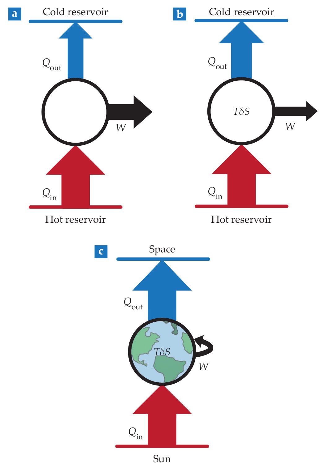
Climate as heat engine. A heat engine produces mechanical energy in the form of work W by absorbing an amount of heat Qin from a hot reservoir (the source) and depositing a smaller amount Qout into a cold reservoir (the sink). (a) An ideal Carnot heat engine does the job with the maximum possible efficiency. (b) Real heat engines are irreversible, and some work is lost via irreversible entropy production TδS. (c) For the climate system, the ultimate source is the Sun, with outer space acting as the sink. The work is performed internally and produces winds and ocean currents. As a result, Qin = Qout.
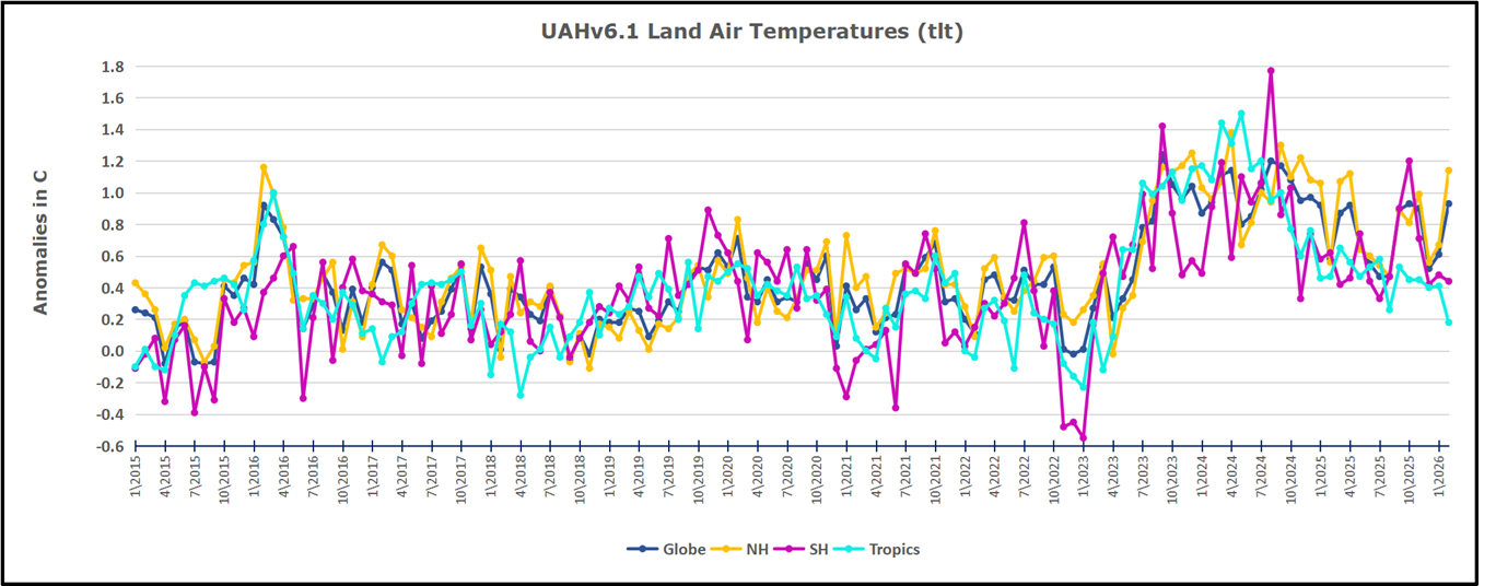
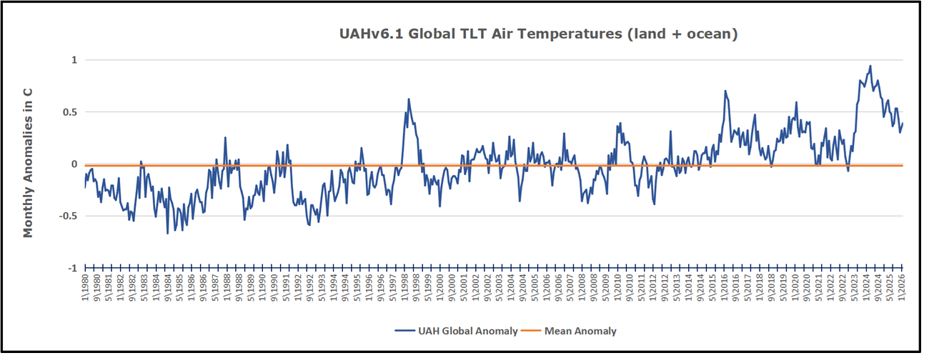
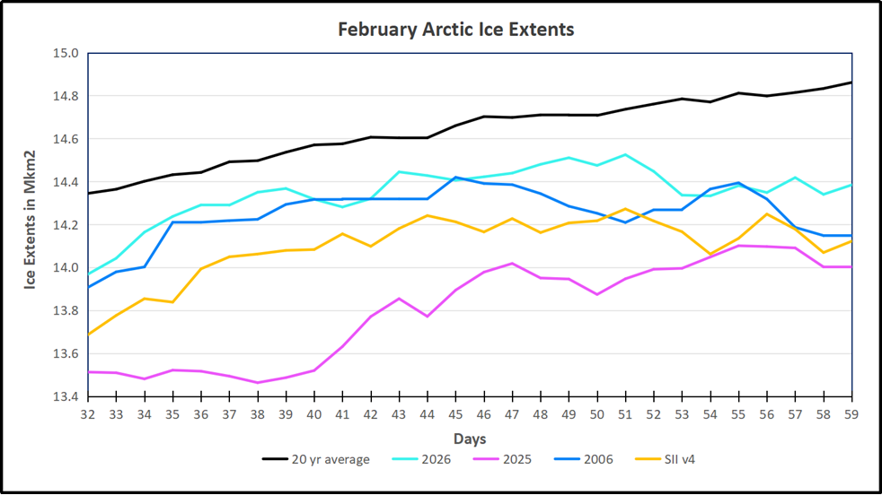
Update 2026
Kevin Mooney writes at Real Clear Energy Trump Is Right: Science Demands That We Overturn the ‘Endangerment Finding’ Excerpts in italics with my bolds.
Taking on the climate establishment with research that debunks the media narrative.
Science is on the side of the Trump administration’s efforts to unwind the U.S. from costly climate regulations—much to the consternation of major media platforms that peddle unfounded, politically motivated assertions.
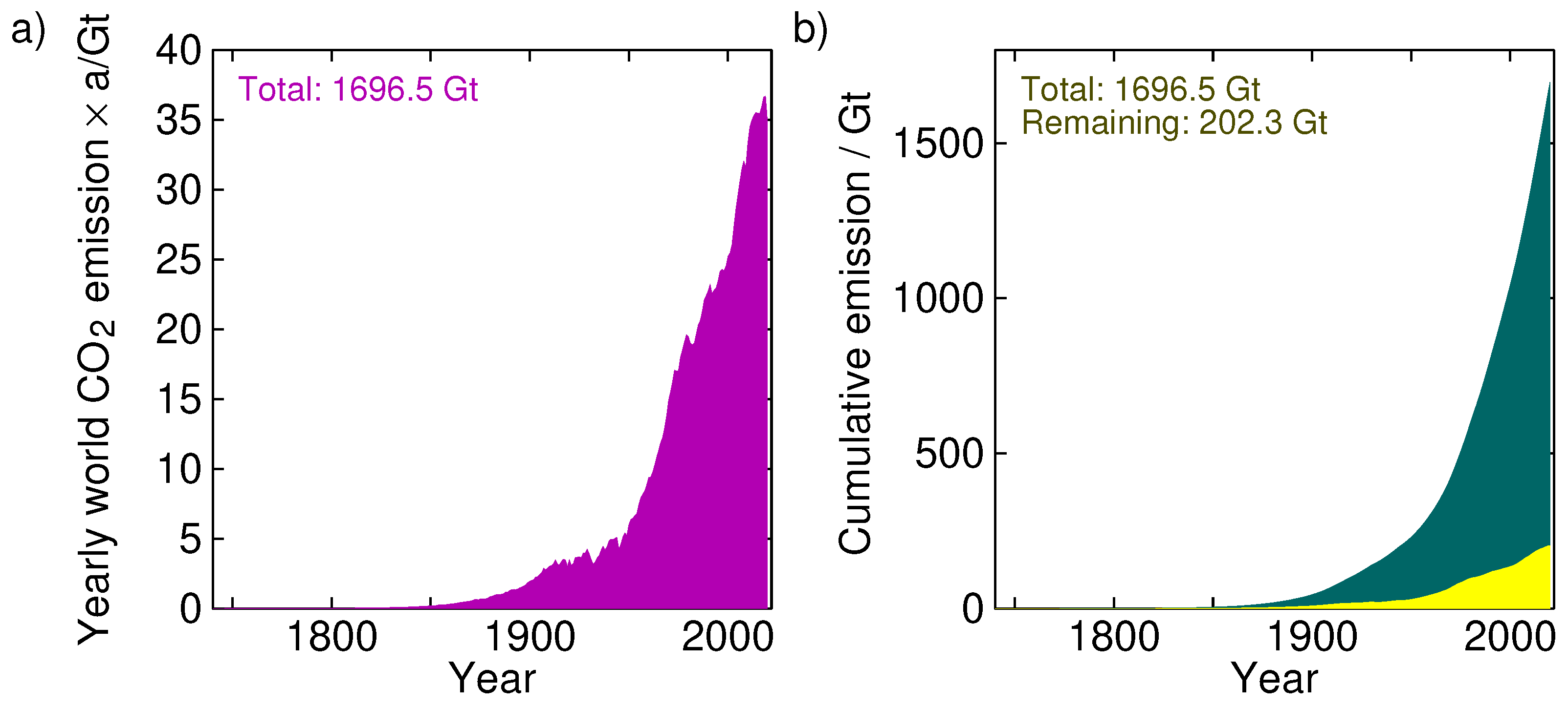
That’s why fresh research and updated findings into the impact of carbon dioxide emissions should figure more prominently into an otherwise laudatory and audacious White House strategy to repeal the 2009 endangerment finding. In my new book, Climate Porn: How and Why Anti-Population Zealots Fabricate Science, while Targeting American Capitalism, Freedom, and Independence, I review the science and common sense that reiterates CO2 is a naturally occurring, highly beneficial compound. Indeed, it is critical to life on Earth. And yet, the Obama administration saw fit to declare CO2 a “pollutant” in its endangerment finding, which found that CO2 poses a threat to public health and welfare. This enabled the EPA to unleash a wave of costly climate regulations.
Trump, Zeldin, Wright, and crew should not just rely on legal arguments, but rather double down on the science as they take on the endangerment finding. Posterity will thank them.
Recent Research Discredits Climatists’ Fearful Claims
In light of the above context, I am posting a recent and significant rebuttal of the IPCC “consensus” science that is full of holes like swiss cheese. Ad Huijser recently published a paper explaining why IPCC claims about global warming are contradicted by observations of our Earth thermal system including a number of internal and external subsytems. The title Global Warming and the “impossible” Radiation Imbalance links to the pdf. This post is a synopsis to present the elements of his research findings, based on the rich detail, math and references found in the document. Excerpts in italics with my bolds and added images. H/T Kenneth Richard and No Tricks Zone.
Abstract
Any perturbation in the radiative balance at the top of the atmosphere (TOA) that induces a net energy flux into- or out of Earth’s thermal system will result in a surface temperature response until a new equilibrium is reached. According to the Anthropogenic Global Warming (AGW) hypothesis which attributes global warming solely to rising concentrations of Greenhouse gases (GHGs), the observed increase in Earth’s radiative imbalance is entirely driven by anthropogenic GHG-emissions.
However, a comparison of the observed TOA radiation imbalance with the assumed GHG forcing trend reveals that the latter is insufficient to account for the former. This discrepancy persists even when using the relatively high radiative forcing values for CO2 adopted by the Intergovernmental Panel on Climate Change (IPCC), thereby challenging the validity of attributing recent global warming exclusively to human-caused GHG emissions.
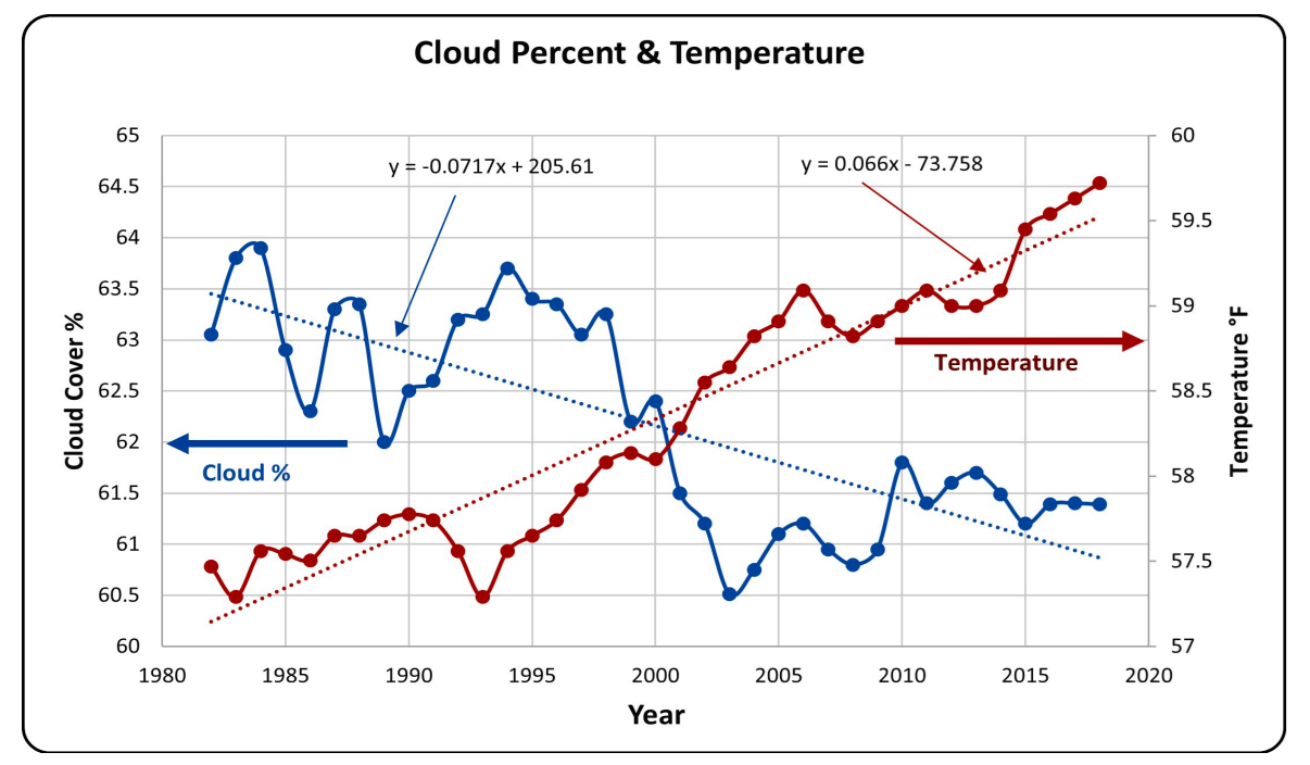
In this paper, Earth’s climate system is analyzed as a subsystem of the broader Earth Thermal System, allowing for the application of a “virtual balance” approach to distinguish between anthropogenic and other, natural contributions to global warming. Satellite-based TOA radiation data from the CERES program (since 2000), in conjunction with Ocean Heat Content (OHC) data from the ARGO float program (since 2004), indicate that natural forcings must also play a significant role. Specifically, the observed warming aligns with the net increase in incoming shortwave solar radiation (SWIN), likely due to changes in cloud cover and surface albedo. Arguments suggesting that the SWIN trend is merely a feedback response to GHG-induced warming are shown to be quantitatively insufficient.
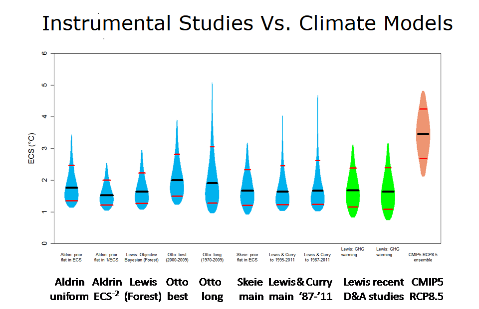
This analysis concludes that approximately two-thirds of the observed global warming must be attributed to natural factors that increase incoming solar radiation, with only one-third attributable to rising GHG-concentrations. Taken together, these findings imply a much lower climate sensitivity than suggested by IPCC-endorsed Global Circulation Models (GCMs).
Introduction
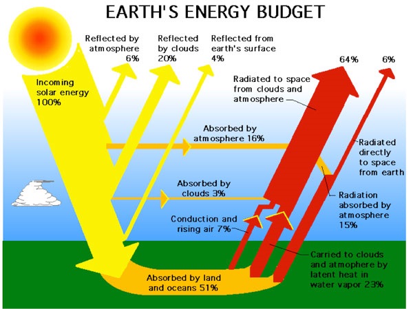
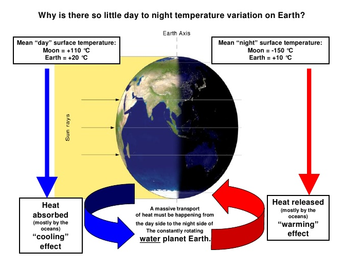
On a global scale and over longer periods of time, the average surface temperature of our climate system reacts similarly to that of a thermal system such as a pot of water on a stove: when the incoming heat is steady and below boiling, the system stabilizes when the heat loss (via radiation and convection) equals the input. Analogously, Earth’s surface-atmosphere interface is the main absorber and emitter of heat. Reducing the “flame” (solar input) leads to cooling, regardless of the total heat already stored in the system. The system’s average temperature will drop as well, as soon as the heating stops. So, no sign of any “warming in the pipeline” for such a simple system.
The two transport mechanisms, air and ocean, operate on different timescales. Air has a low specific heat capacity, but high wind speeds make it a fast medium for heat transfer. Oceans, by contrast, have a high specific heat capacity but move more slowly. The Atlantic Meridional Overturning Circulation (AMOC) with the well-known Gulf Stream carrying warm water from south to north, can reach speeds up to about 3 m/s. But its warm current remains largely confined to surface layers due to limited solar radiation penetration and gravity-induced stratification. With a path-lengths of up to 8,000 km and an average speed of 1.5 m/s, ocean heat takes approximately 2 months to travel from the Gulf of Mexico to the Arctic. This is comparable to the 1 to 2 months delay between solar input and temperature response in the annual cycle, suggesting that oceanic heat transport is part of the climate system’s normal operation. Climate adaptation times from anthropogenic influences are estimated at 3 to 5 years. If “warming in the pipeline” exists, it must be buried in the much colder, deeper ocean layers.
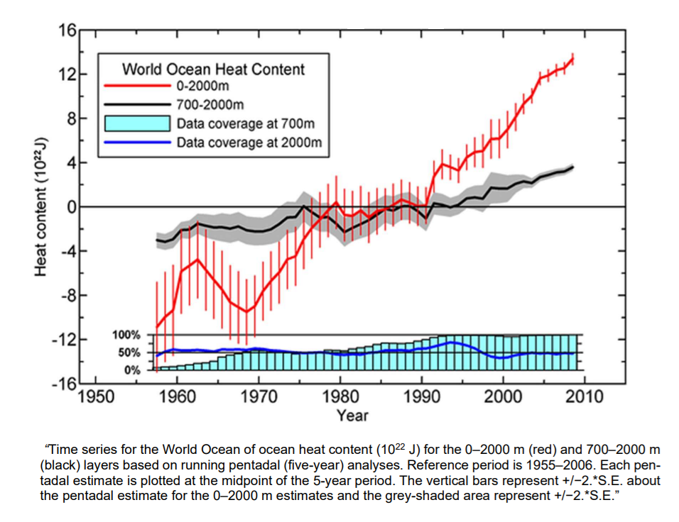
ARGO float data since 2004 show substantial annual increases in Ocean Heat Content (OHC), sometimes expressed in mind-boggling terms such as 10²² joules per year (see Fig.1). While this may sound alarming [1,2], when converted to flux, it represents less than 1 W/m², a mere 0.6% of the average 160 W/m² of absorbed solar energy at the surface. All the rest is via evaporation, convection and ultimately by radiation sent back to space after globally being redistributed by wind and currents.
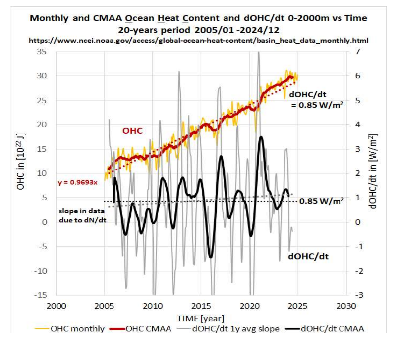
Fig. 1. Ocean Heat Content (OHC) anomaly from 0–2000 meters over time, shown as 3-month and annual moving averages (CMAA), along with their time derivatives. Notable are the relatively large variations, likely reflecting the influence of El Niño events. The average radiative imbalance at the top of the atmosphere (TOA), estimated at 0.85 W/m², corresponds approximately to the midpoint of the time series (around 2015). Data: https://www.ncei.noaa.gov/access/global-ocean-heat-content/basin_heat_data.html [7].
Estimating our climate’s thermal capacity CCL
The rather fast responses of our climate indicates that the thermal capacity of our climate must be much less than the capacity of the entire Earth thermal system. This climate heat capacity CCL depends on how sunlight is being absorbed, how that heat is transferred to the atmosphere and which part of it is being stored in either land or ocean.
At continental land-area, sunlight is absorbed only at the very surface where the generated heat is also in direct contact with the atmosphere. Seasonal temperature variations don’t penetrate more than 1 to 2 meters deep in average and as a consequence, storage of heat is relatively small. Sunlight can penetrate pure water to several hundred meters deep, but in practice, penetration in the oceans is limited by scattering and absorption of organic and inorganic material. A good indication is the depth of the euphotic zone where algae and phytoplankton live, which need light to grow. In clear tropical waters where most of the sunlight hits our planet, this zone is 80 to 100 m deep [12].
Another important factor in our climate’s heat capacity is how this ocean layer of absorbed heat is in contact with the atmosphere. Tides, wind, waves and convection continuously mix the top layer of our oceans, by which heat is easily exchanged with the atmosphere. This mixed-layer is typically in the order of 25 – 100 m, dependent on season, latitude and on the definition of “well mixed” [13]. Below this ~100 m thick top-layer, where hardly any light is being absorbed and the mixing process has stopped, ocean temperatures drop quickly with depth. As the oceans’ vertical temperature gradient at that depth doesn’t support conductive nor convective heat flows going upward, climate processes at the surface will thus become isolated from the rest of the Earth’ thermal system.
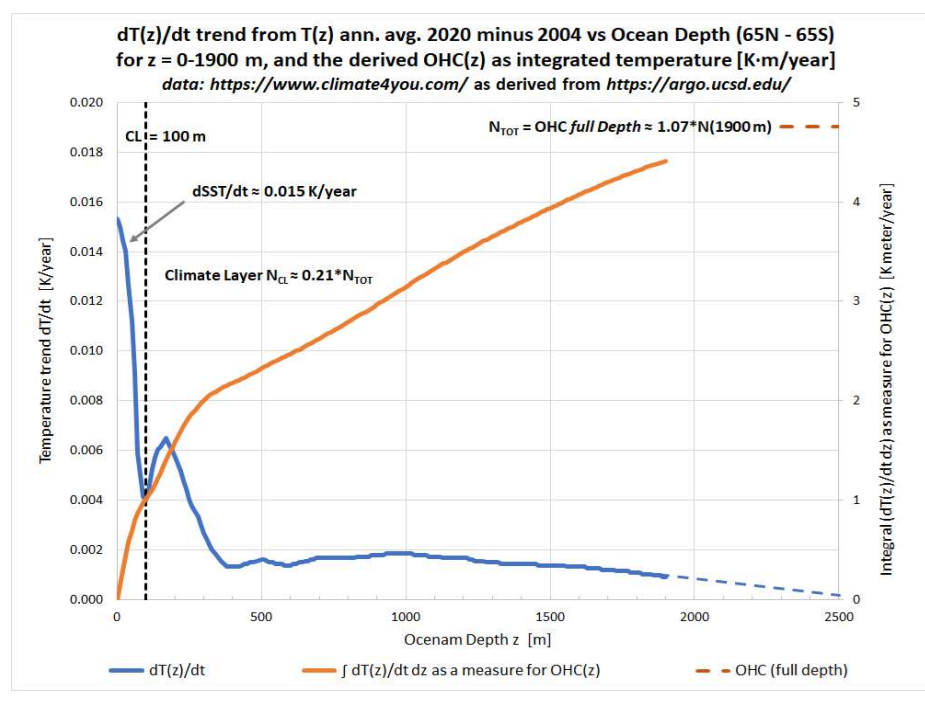
Figure 4 with the Change in Ocean Heat Content vs. Depth over the period 2004 – 2020 obtained via the ARGO-floats [6,14], offers a good indication for the average climate capacity CCL. It shows the top layer with a high surface temperature change according to the observed global warming rate of about 0.015 K/year, and a steep cut off at about 100 m depth in line with the explanation above. Below the top layer, temperature effects are small and difficult to interpret, probably due to averaging over all kinds of temperature/depth profiles in the various oceans ranging from Tropical- to Polar regions.
In case of a “perfect” equilibrium (N = 0, dTS/dt = 0), all of the absorbed sunlight up to about 100 m deep, has to leave on the ocean-atmosphere interface again. However, deep oceans are still very cold with a stable, negative temperature gradient towards the bottom. This gradient will anyhow push some of the absorbed heat downwards. Therefore, even at a climate equilibrium with dTS/dt= 0, we will observe N > 0. With the large heat capacity of the total ocean volume, that situation will not change easily, as it takes about 500 years with today’s N ≈ +1 W/m2 to raise its average temperature just 1°C.
The Earth’s climate system can thus be regarded as a subset of the total Earth’s thermal system (ETS) responding to different relaxation times. The climate relaxes to a new equilibrium within 3–5 years, while the deeper oceans operate on multidecadal or even longer timescales, related to their respective thermal capacities C for the ETS, and CCL for the climate system.
The (near) “steady state” character of current climate change
Despite the ongoing changes in climate, the current state can be considered a “near” steady-state. The GHG forcing trend has been pretty constant for decades. Other forcings, primarily in the SW channel, are also likely to change slowly and can be approximated as having constant trends over decadal timescales. Similarly, despite yearly fluctuations, the surface temperature trend has remained fairly stable since 2000.
This analysis strengthens the conclusion that the increase in both N(t) and N0(t) are not a direct consequence of greenhouse gas emissions, but rather of enhanced forcing in the SW-channel.
The preceding analysis highlights how the IPCC’s assumptions diverge significantly from observed reality. While the IPCC model components may collectively reproduce the observed warming trend, they fail to individually align with key observational data, in particular the Ocean Heat Content.
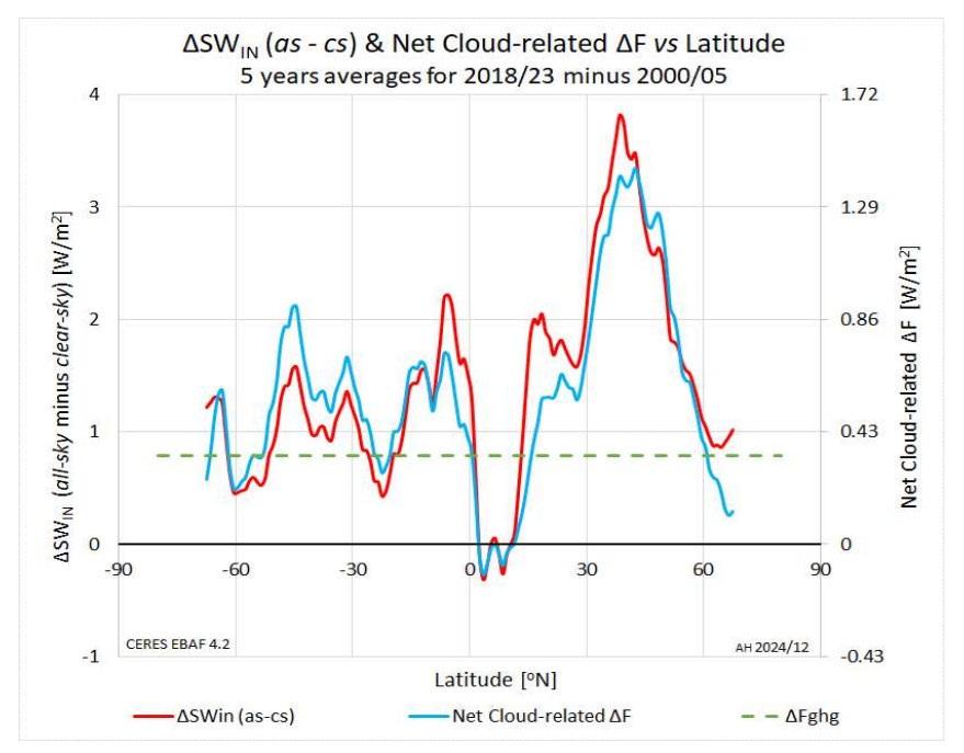
Figure 6 also illustrates that changes in cloudiness are more pronounced on the Northern Hemisphere, especially at mid-latitudes and over Western Europe. For example, the Dutch KNMI weather-station at Cabauw (51.87°N, 4.93oE), where all ground-level radiation components are monitored every 10 minutes, recorded an increase in solar radiation of almost +0.5 W/m²/year since 2000 [26]. Applying the 0.43 net-CRE factor (conservative for this latitude), we estimate a local forcing trend dFSW/dt ≈ 0.2 W/m²/year. This is an order of magnitude larger than the GHG forcing (0.019–0.037 W/m²/year). Even with the IPCC values, GHGs can just account for about 16% of the warming at this station. The average temperature trend for this rural station located in a polder largely covered by grassland, is with ~ +0.043 K/year almost 3x the global average. This, nor the other trends mentioned above can be adequately explained by the IPCC’s GHG-only model.
The IPCC places strong emphasis on the role of climate feedbacks in amplifying the warming effect of greenhouse gases (GHGs) [8]. These feedbacks are considered secondary consequences of Anthropogenic Global Warming, driven by the initial temperature increase from GHGs. Among them, Water-Vapor feedback is the most significant. A warmer atmosphere holds more water vapor (approximately +7%/K) and since water vapor is a potent GHG, even a small warming from CO2 can amplify itself through enhanced evaporation.
Other feedbacks recognized by the IPCC include Lapse Rate, Surface Albedo, and Cloud feedbacks [8], all of which are inherently tied to the presence and behavior of water in its various phases. Therefore, these feedbacks are natural responses to temperature changes, regardless of the original cause of warming, be it GHGs, incoming solar variability, or internal effects. They are not additive components to natural climate sensitivity, as treated by the IPCC, but rather integral parts of it [4].
This analysis reinforces a fundamental point: climate feedbacks are not external modifiers of climate sensitivity; rather, they are inherent to the system. Their combined effect is already embedded in the climate response function. The IPCC’s treatment of feedbacks as additive components used to “explain” high sensitivities in GCMs is conceptually flawed. Physically, Earth’s climate is governed by the mass balance of water in all its phases: ice, snow, liquid, vapor, and clouds. The dynamics between these phases are temperature-sensitive, and they constitute the feedback processes. Feedbacks aren’t just add-ons to the climate system, they are our climate.
Ocean Heat Content increase
In the introduction, the “heat in the pipeline” concept: the idea that heat stored in the deep, cold ocean layers could later resurface to significantly influence surface temperatures, was challenged. Without a substantial decrease in surface temperatures to reverse ocean stratification, this seems highly unlikely. Large and rapid temperature fluctuations during the pre-industrial era with rates up to plus, but also minus 0.05 K/year over several decennia as recorded in the Central England Temperature (CET) series [27], more than three times the rate observed today, further undermine the notion of a slow-release heat mechanism dominating surface temperature trends.
Ocean Heat Content must be related to solar energy. It is the prime source of energy heating the Earth thermal system. Almost 1 W/m2 of that 240 W/m2 solar flux that is in average entering the system, is presently remaining in the oceans. This is an order of magnitude larger than the estimated 0.1 W/m2 of geothermal heat upwelling from the Earth inner core [11]. Extra greenhouse gasses don’t add energy to the system, but just obstruct cooling. As shown in Section 5.3, this accounts for a radiation imbalance offset τ dFGHG/dt, or equivalent to a contribution to dOHC/dt of only about 0.08 W/m2.
.
As redistribution of “heat in the pipeline” will not change the total OHC, roughly 3/4 of the observed positive trend in OHC must at least be attributed to rising solar input. The oceans act in this way as our climate system’s thermal buffer. It will mitigate warming during periods of increased solar input and dampen cooling when solar input declines, underscoring its critical role in Earth’s climate stability.
The strong downwards slope in the OHC before 1970 confirms the observation in Section 5.4 and expressed by (12) that around the turning point t = ζ, the forcing trend in the SW-channel had to be negative. Moreover, the rather slowly increasing 700-2000m OHC data in Fig.7 indicate that most of the fluctuations have occurred relatively close to the surface. Heat from e.g. seafloor volcanism as “warming from below”, is expected to show up more pronounced in this 700-2000m OHC-profile. Although we cannot rule out geothermal influences [29], this observation makes them less likely.

ERBE measurements of radiative imbalance.
As the OHC seems to be primarily coupled to SWIN, the most plausible cause would involve rapid changes in SW-forcing. A sudden drop in cloud-cover might explain such changes, but no convincing observations could be found for the 1960-1980 period. Alternatively, changes in the latitudinal distribution of cloud-cover as illustrated by Fig.6, can result in similar radiative impacts due to the stark contrast between a positive radiation imbalance in the Tropics and a very negative imbalance at the Poles. The ENSO-oscillations in the Pacific Ocean around the equator are a typical example for such influences, as also illustrated in Fig.3 [10]. Shifts in cloud distribution are linked to changes in wind patterns and/or ocean currents, reinforcing the idea as indicated in Section 1, that even minor disruptions in horizontal heat transport can trigger major shifts in our climate’s equilibrium [29, 30]. Sharp shifts in Earth’s radiation imbalance like the one around 1970 as inferred from Fig.7, may even represent one of those alleged tipping points. But in this case, certainly not one triggered by GHGs. Ironically, some climate scientists in the early 1970s predicted an impending (Little) Ice Age [31].
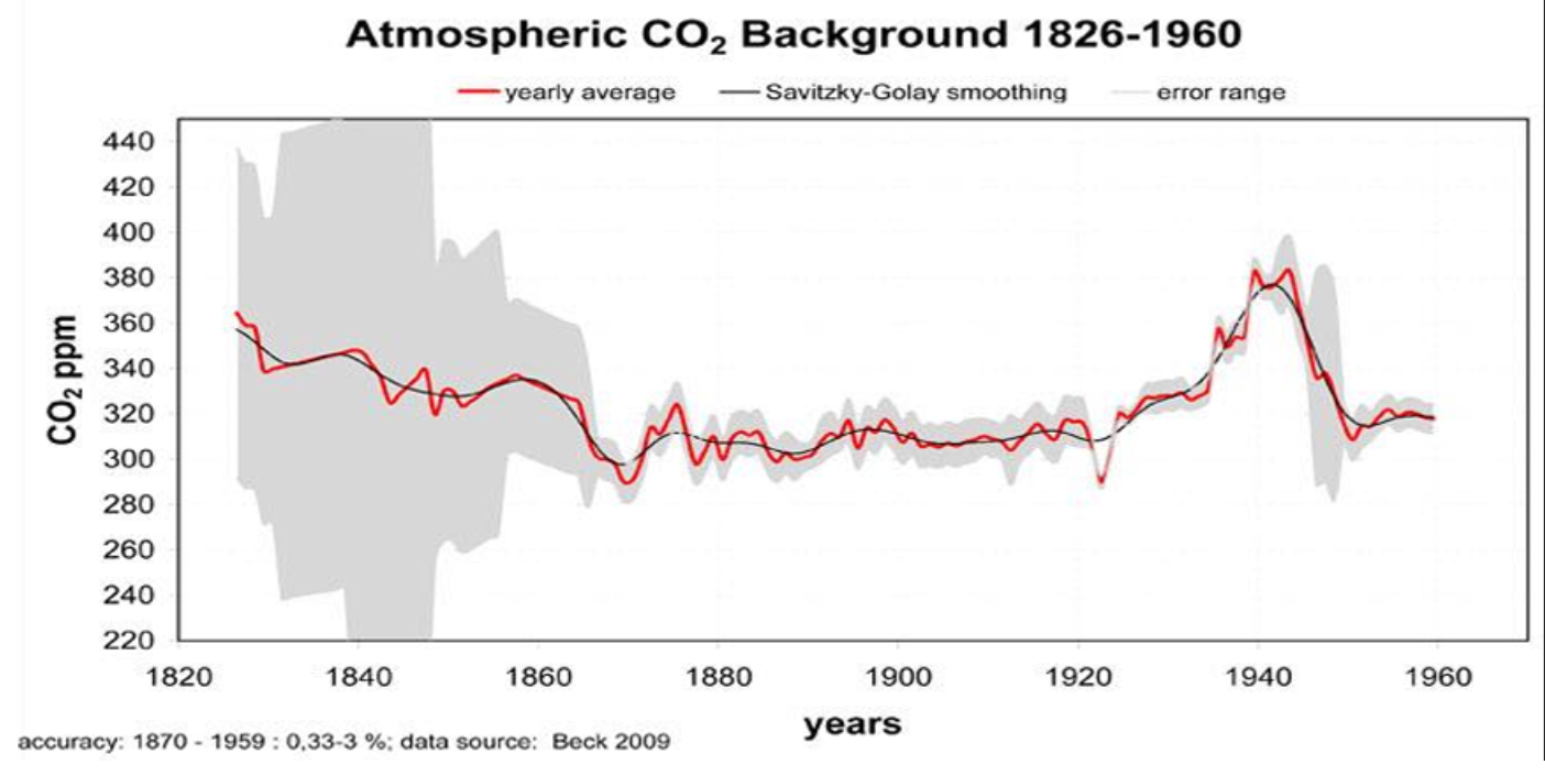
While additional data (e.g. radiation measurements) are needed to draw firm conclusions, the available evidence already challenges the prevailing GHG-centric narrative again. GHG emissions, with their near constant forcing rate, cannot account for the timing nor the magnitude of historical OHC trends, as NOAA explicitly suggests [32]. Similarly, claims by KNMI that “accelerations” in radiation imbalance trends are GHG-driven [1], are not supported by data. And finally, the alarms around “heat in the pipeline” must be exaggerated if not totally misplaced. Given the similarities in radiation imbalance and GHG forcing rates around 1970 with today’s situation, we must conclude that this assumed heat manifested itself at that time apparently as “cooling in the pipeline”.
However, warnings for continued warming even if we immediately stop now with emitting GHGs are nevertheless, absolutely justified. Only, it isn’t warming then from that heat in the pipeline due to historical emissions that will boost our temperatures. Warming will continue to go on as long as natural forcings will be acting. These are already today’s dominant drivers behind global temperature trends. And unfortunately, they will not be affected by the illusion of stopping global warming as created by implementing Net-Zero policies.
Summary and conclusions
This analysis demonstrates that a global warming scenario driven solely by greenhouse gases (GHGs) is inconsistent with more than 20 years of observations from space and of Ocean Heat Content. The standard anthropogenic global warming (AGW) hypothesis, which attributes all observed warming to rising GHG concentrations, particularly CO2, cannot explain the observed trends. Instead, natural factors, especially long-term increase in incoming solar radiation, appear to play a significant and likely dominant role in global warming since the mid-1970s.
The observed increase in incoming solar radiation cannot be accounted for by the possible anthropogenic side effects of Albedo- and Cloud-feedback. All evidence points to the conclusion that this “natural” forcing with a trend of about 0.035 W/m2/year is equal to, or even exceeds the greenhouse gas related forcing of about 0.019 W/m2/year. Based on these values, only 1/3rd of the observed temperature trend can be of anthropogenic origin. The remaining 2/3rd must stem from natural changes in our climate system, or more broadly, in our entire Earth’ thermal system.
Moreover, the observed increase in Earth’s radiation imbalance appears to be largely unrelated to GHGs. Instead, it correlates strongly with natural processes driving increased incoming solar radiation. Claims of “acceleration” in the radiation imbalance due to GHG emissions are not supported by the trend in accurately measured GHG concentrations. If any acceleration in global warming is occurring, it is almost certainly driven by the increasing flux of solar energy—an inherently natural phenomenon not induced by greenhouse gases.
In summary, this analysis challenges the notion that GHGs are the primary drivers of recent climate change. It underscores the importance of accounting for natural variability, especially in solar input, when interpreting warming trends and evaluating climate models.
Note: Dr. Ad Huijser, physicist and former CTO of Philips and director of the Philips Laboratories, describes himself as “amateur climatologist”. However his approach to climate physics is quite professional, I think.

See Also:
Our Atmospheric Heat Engine


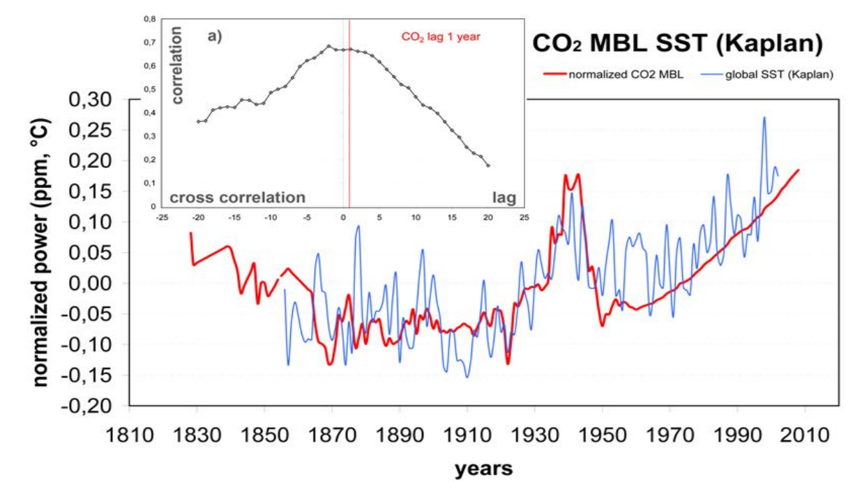
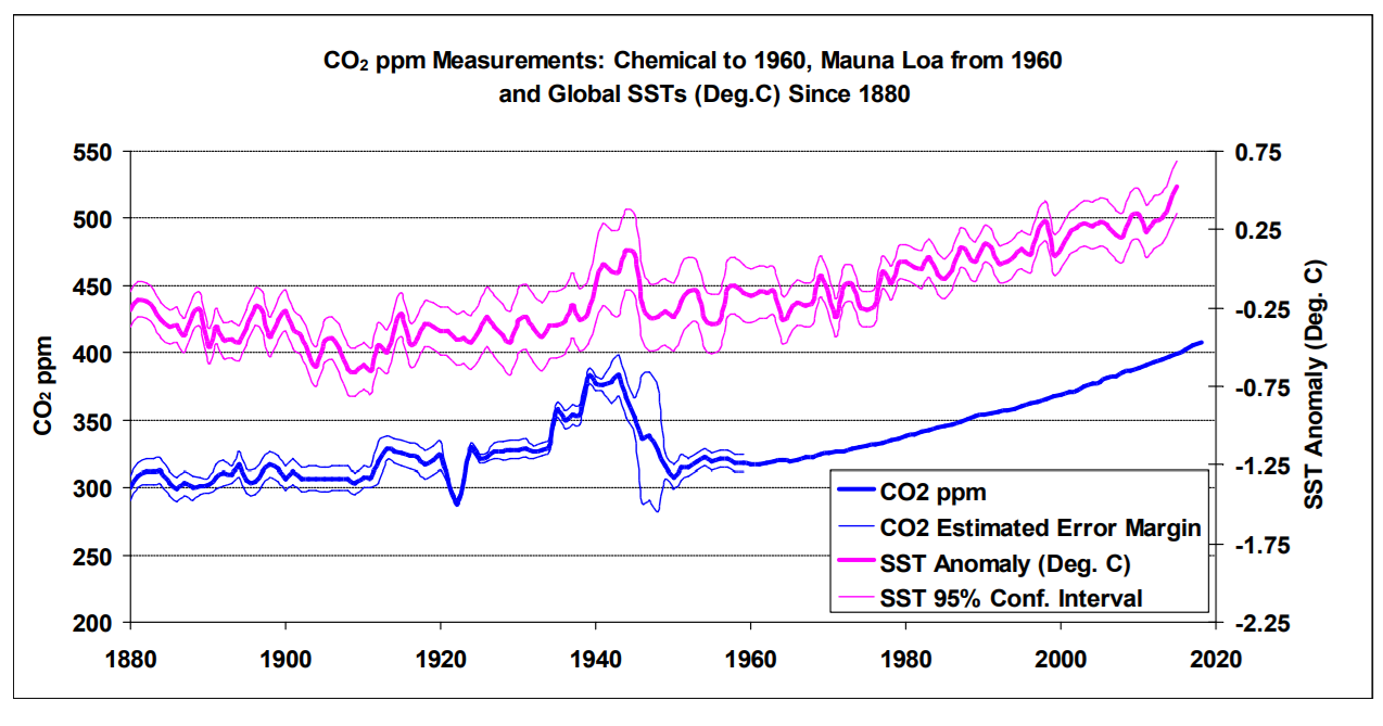


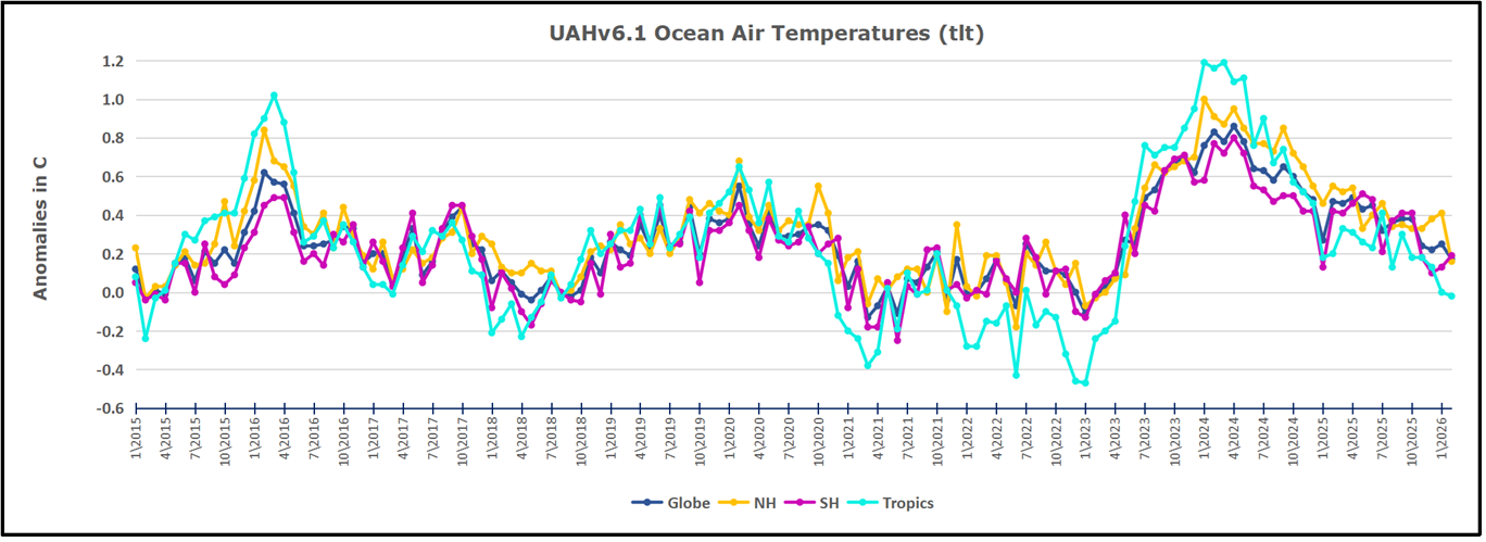


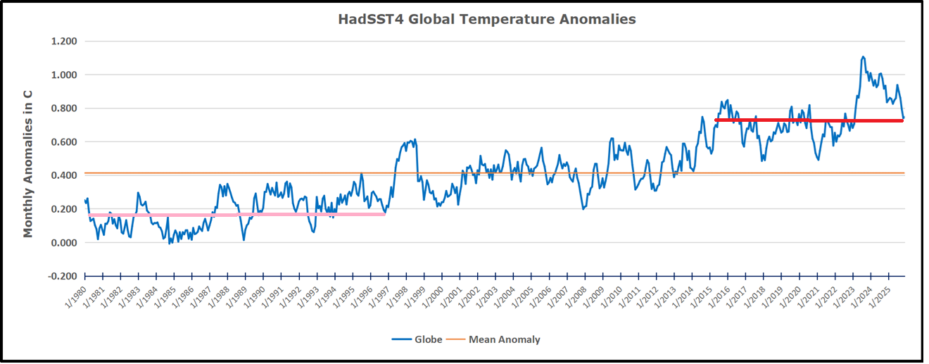
 The best context for understanding decadal temperature changes comes from the world’s sea surface temperatures (SST), for several reasons:
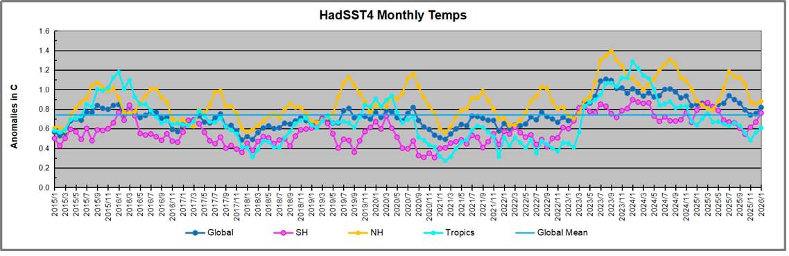


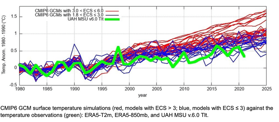


 Moreover, despite ongoing controversy surrounding long-term solar variability, current GCMs are typically forced with solar reconstructions that exhibit extremely low secular variability. This helps explain why these models attribute nearly 0 °C of the observed post 1850–1900 warming to solar changes and simultaneously fail to reproduce the millennial-scale oscillations evident in paleoclimate records.