
Previous posts (linked at end) discuss how the climate model from RAS (Russian Academy of Science) has evolved through several versions. The interest arose because of its greater ability to replicate the past temperature history. The model is part of the CMIP program which will soon go the next step to CMIP7, and is one of the first to test with a new climate simulation.
This synopsis is made possible thanks to the lead author, Evgeny M. Volodin, providing me with a copy of the article published May 11, 2023 in Izvestiya, Atmospheric and Oceanic Physics. Those with institutional research credentials can access the paper at Simulation of Present-Day Climate with the INMCM60 Model by E. M. Volodin, et al. (2023). Excerpts are in italics with my bolds and added images and comment.
Abstract
A simulation of the present-day climate with a new version of the climate model developed at the Institute of Numerical Mathematics of the Russian Academy of Sciences (INM RAS) is considered. This model differs from the previous version by a change in the cloud and condensation scheme, which leads to a higher sensitivity to the increase in СО2. The changes are also included in the calculation of aerosol evolution, the aerosol indirect effect, land snow, atmospheric boundary-layer parameterization, and some other schemes.
The model is capable of reproducing near-surface air temperature, precipitation, sea-level pressure, cloud radiative forcing, and other parameters better than the previous version. The largest improvement can be seen in the simulation of temperature in the tropical troposphere and at the polar tropopause and surface temperature of the Southern Ocean. The simulation of climate changes in 1850 2021 by the two model versions is discussed.
Introduction
A new version has been developed on the basis of the climate system model described in [1]. It was shown [2] that introducing changes only to the cloud parameterization would produce climate models with different equilibrium sensitivities to a doubling of СО2, in a range of 1.8 to 4.1 K. The INMCM48 version has the lowest sensitivity of 1.8 K among Coupled Model Intercomparison Project Phase 6 (CMIP6) models. The natural question then arises as to how parameterization changes that increase the equilibrium sensitivity affect the simulation of modern climate and of its changes observed in recent decades.
The INMCM48 version simulates modern climate quite well, but it has some systematic biases common to many of the current climate models, and biases specific only to this model. For example, most climate models overestimate surface temperatures and near surface air temperatures at southern midlatitudes and off the east coast of the tropical Pacific and Atlantic oceans and underestimate surface air temperatures in the Arctic (see, e.g., [3]). A typical error of many current models, as well as of INMCM48, is the cold polar tropopause and the warm tropical tropopause, resulting in an overestimation of the westerlies in the midlatitude stratosphere. Possible sources of such systematic biases are the errors in the simulation of cloud amount and optical properties.
In the next version, therefore, changes were first made in cloud parameterization. Furthermore, the INMCM48 exhibited systematic biases specific solely to it. These are, for example, the overestimation of sea-level pressure, as well as of geopotential at any level in the troposphere, over the North Pacific. The likely reason for such biases seems to be related to errors in the heat sources located southward, over the tropical Pacific.
In this study, it is shown how changes in physical parameterizations,
including clouds, affect systematic biases in the simulation of
modern climate and its changes observed in recent decades.
Model and Numerical Experiments
The INMCM60 model, like the previous INMCM48 [1], consists of three major components: atmospheric dynamics, aerosol evolution, and ocean dynamics. The atmospheric component incorporates a land model including surface, vegetation, and soil. The oceanic component also encompasses a sea-ice evolution model. Both versions in the atmosphere have a spatial 2° × 1° longitude-by-latitude resolution and 21 vertical levels up to 10 hPa. In the ocean, the resolution is 1° × 0.5° and 40 levels.
The following changes have been introduced into the model
compared to INMCM48.
Parameterization of clouds and large-scale condensation is identical to that described in [4], except that tuning parameters of this parameterization differ from any of the versions outlined in [3], being, however, closest to version 4. The main difference from it is that the cloud water flux rating boundary-layer clouds is estimated not only for reasons of boundary-layer turbulence development, but also from the condition of moist instability, which, under deep convection, results in fewer clouds in the boundary layer and more in the upper troposphere. The equilibrium sensitivity of such a version to a doubling of atmospheric СО2 is about 3.3 K.
The aerosol scheme has also been updated by including a change in the calculation of natural emissions of sulfate aerosol [5] and wet scavenging, as well as the influence of aerosol concentration on the cloud droplet radius, i.e., the first indirect effect [6]. Numerical values of the constants, however, were taken to be a little different from those used in [5]. Additionally, the improved scheme of snow evolution taking into account refreezing and the calculation of the snow albedo [7] were introduced to the model. The calculation of universal functions in the atmospheric boundary layer in stable stratification has also been changed: in the latest model version, such functions assume turbulence at even large gradient Richardson numbers [8].
A numerical model experiment to simulate a preindustrial climate was run for
180 years, not including the 200 years when equilibrium was reached.
All climate forcings in this experiment were held at their 1850 level. Along with a preindustrial experiment, a numerical experiment was run to simulate climate change in 1850–2029, for which forcings for 1850–2014 were prescribed consistent with observational estimates [9], while forcings for 2015–2029 were set according to the Shared Socioeconomic Pathway (SSP3-7.0) scenario [10].
To verify the simulation of present-day climate, the data from the experiment with a realistic forcing change for 1985–2014 were used and compared against the European Centre for Medium-Range Weather Forecasts (ECMWF) Reanalysis fifth generation (ERA5) data [11], the Global Precipitation Climatology Project, version 2.3 (GPCP 2.3) precipitation data [12], and the Clouds and the Earth’s Radiant Energy System (CERES) Energy Balanced and Fitted Edition 4.1 (CERES-EBAF 4.1) top-of-atmosphere (TOA) outgoing radiation fluxes [13].
The root-mean-square deviation of the annual and monthly averages of modeled and observed fields was used as a measure for the deviation of model data from observations, for which the observed fields were interpolated into a model grid. For calculating the sea-level pressure and 850-hPa temperature errors, grid points with a height over 1500 m were excluded. The modeled surface air temperatures were compared with the Met Office Hadley Center/Climatic Research Unit version 5 (HadCRUT5) dataset [14].
Results
Below are some results of the present-day climate simulation. Because changes in the model were introduced mainly into the scheme of atmospheric dynamics and land surface and there were no essential changes in the oceanic component, we shall restrict our discussion to atmospheric dynamics.
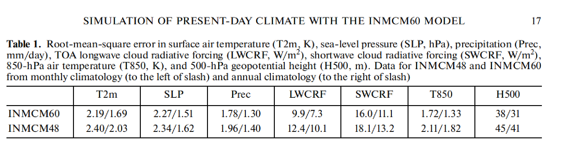
Table 1 demonstrates that the norms of errors in most fields were reduced. Changing the calculation of cloud cover and properties has improved the cloud radiative forcing, and the norm of errors for both longwave and shortwave forcing decreased by 10–20% in the new version compared to its predecessor. The global average of short-wave cloud radiative forcing is –47.7 W/m2 in the new version, –40.5 W/m2 in the previous version, and about –47 W/m2 in CERES-EBAF. The average TOA longwave radiative forcing is 29.5 W/m2 in the new version, 23.2 W/m2 in the previous version, and 28 W/m2 in CERES-EBAF. Thus, the average longwave and shortwave cloud radiative forcing in the new model version has proven to be much closer to observations than in the previous version.
From Table 1, the norm of the systematic bias has decreased significantly for 850-hPa temperatures and 500-hPa geopotential height. It was reduced mainly because average values of these fields approached observations, whereas the averages of both fields in INMCM48 were underestimated.
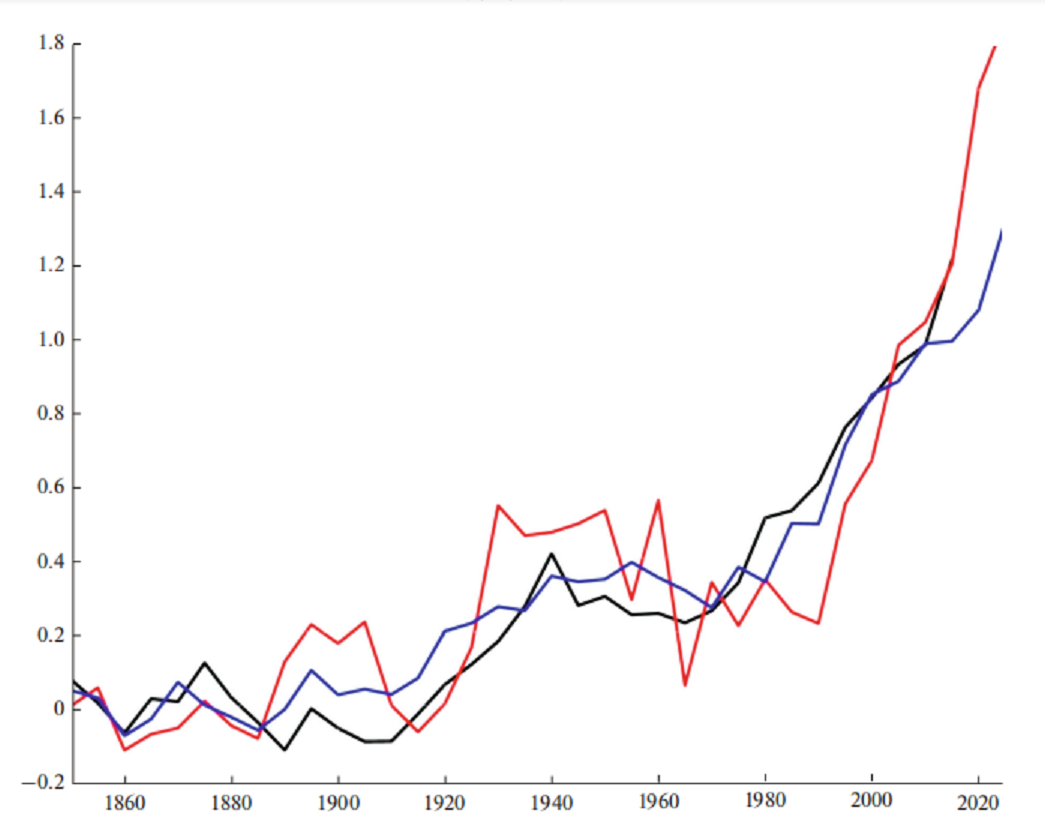
Figure 3 Volodin et al (2023)
We now consider the simulation of climate changes for 1850–2021. The 5-year mean surface temperature from HadCRUT5 (black), INMCM48 (blue), and INMCM60 (red) is shown in Fig. 3. The average for the period 1850 to 1899 is subtracted for each of the three datasets. The model data are slightly extended to the future, so that the most recent value matches the 2025–2029 average. It can be seen that warming in both versions by 2010 is about 1 K, approximately consistent with observations. The observed climate changes, such as the warmer 1940s and 1950s and the slower warming, or even a small cooling, in the 1960s and 1970s, are also obtained in both model versions. However, the warming after 2010–2014 turns out to be far larger in the new version than in the previous one, with differences reaching 0.5 K in 2025–2029. The discrepancies between the two versions are most distinct in the rate of temperature rise from 1990–1994 to 2025–2029. In INMCM48, the temperature rises by about 0.8 K, while the increase for INMCM60 is about 1.5 K. The discrepancy appears to have been caused primarily by a different sensitivity of the models, but a substantial contribution may also come from natural variability, so a more reliable conclusion could be made only by running ensemble numerical experiments.
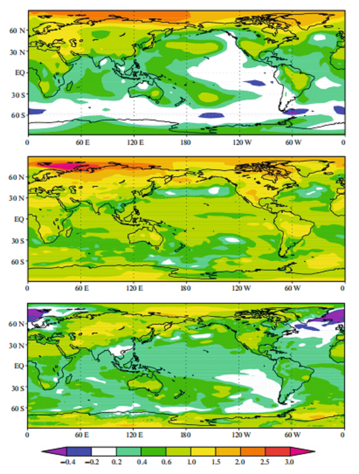
Figure 4 Volodin et al. (2023)
Figure 4 displays the difference in surface air temperature from HadCRUT5 (top), the new version (midddle) , and the previous version (bottom) in 2000–2021 and 1979–1999. It is the interval where the warming was the largest, as is seen in Fig. 3. The observational data show that the largest warming, above 2 K, was in the Arctic, there was a warming of about 1 K in the Northern Hemisphere midlatitudes, and there was hardly any warming over the Southern Ocean. The pattern associated with a transition of the Pacific Decadal Oscillation (PDO) from the positive phase to the negative one appears over the Pacific Ocean. The new model version simulates a temperature rise at high and middle northern latitudes more closely to observations, whereas the previous version underestimates the rise in temperature in that region.
At the same time, over the tropical oceans where the observed warming is small, the data from the previous model version agree better with observations, while the new version overestimates warming. Both models failed to reproduce the Pacific Ocean temperature changes resulting from a positive to negative phase transition of PDO, as well as near zero temperature changes at southern midlatitudes. Large differences of temperature change in the Atlantic sector of the Arctic, where there is some temperature decrease in the INMCM48 model and substantial increase in the INMCM60, are most probably caused by natural climate fluctuations in this region, so a reliable conclusion regarding the response of these model versions to observed forcing could also be drawn here only by running ensemble numerical experiments.
Conclusions
The INMCM60 climate model is able to simulate present-day climate better than the previous version The largest decrease can be seen in systematic biases connected with an overestimation of surface temperatures at southern midlatitudes, an underestimation of surface air temperatures in the Arctic, and an underestimation of polar tropopause and tropospheric temperatures in the tropics. The simulation of the cloud radiative forcing has also improved.
Despite different equilibrium sensitivities to doubled СО2, both model versions show approximately the same global warming by 2010–2015, similar to observations. However, projections of global temperature for 2025–2029 already differ between the two model versions by about 0.5 K. A more reliable conclusion regarding the difference in the simulation of current climate changes by the two model versions could have been made by running ensemble simulations, but this is likely to be done later because of the large amount of computational time and computer resources it will take.
My Comments
- Note that INMCM60 runs hotter than version 48 and HadCRUT5. However, as the author points out, this is only a single simulation run, and a truer result will come later from an ensemble of multiple runs. There were several other references to tetnative findings awaiting ensemble runs yet to be done.
For example see the comparable ensemble performance of the previous version (then referred to as INMCM5)

Figure 1. The 5-year mean GMST (K) anomaly with respect to 1850–1899 for HadCRUTv4 (thick solid black); model mean (thick solid red). Dashed thin lines represent data from individual model runs: 1 – purple, 2 – dark blue, 3 – blue, 4 – green, 5 – yellow, 6 – orange, 7 – magenta. In this and the next figures numbers on the time axis indicate the first year of the 5-year mean.
2. Secondly, this study confirms the warming impacts of cloud parameters that appear in all the CMIP6 models. They all run hotter primarily because of changes in cloud settings. The author explains how INMCM60 performance improved in various respects, but it came with increased CO2 sensitivity. That value rose from 1.8C per doubling to 3.3C, shifting the model from lowest to middle of the range of CMIP6 models. (See Climate Models: Good, Bad and Ugly)

Figure 8: Warming in the tropical troposphere according to the CMIP6 models. Trends 1979–2014 (except the rightmost model, which is to 2007), for 20°N–20°S, 300–200 hPa.
3. Thirdly, the temperature record standard has changed with a warming bias. See below from Clive Best comparison between HadCrut 4.6 and HadCrut 5.

The HadCRUT5 data show about a 0.1C increase in annual global temperatures compared to HadCRUT4.6. There are two reasons for this.
The change in sea surface temperatures moving from HadSST3 to HadSST4
The interpolation of nearby station data into previously empty grid cells.
Here I look into how large each effect is. Shown above is a comparison of HadCRUt4.6 with HadCRUT5.
Coincidentally or not, with the temperature standard shifting to HadCrut 5, model parameters shifted to show more warming to match. Skeptics of climate models are not encouraged by seeing warming added into the temperature record, followed by models tuned to increase CO2 warming.
4. The additional warming in both the model and in HadCRUT5 is mostly located in the Arctic. However, those observations include a warming bias derived from using datasets of anomalies rather than actual temperature readings.

Clive Best provides this animation of recent monthly temperature anomalies which demonstrates how most variability in anomalies occur over northern continents.
See Temperature Misunderstandings
The main problem with all the existing observational datasets is that they don’t actually measure the global temperature at all. Instead they measure the global average temperature ‘anomaly’. . .The use of anomalies introduces a new bias because they are now dominated by the larger ‘anomalies’ occurring at cold places in high latitudes. The reason for this is obvious, because all extreme seasonal variations in temperature occur in northern continents, with the exception of Antarctica. Increases in anomalies are mainly due to an increase in the minimum winter temperatures, especially near the arctic circle.
A study of temperature trends recorded at weather stations around the Arctic showed the same pattern as the rest of NH. See Arctic Warming Unalarming
5. The CMIP program specifies that participating models include CO2 forcing and exclude solar forcing. Aerosols are the main parameter for tuning models to match. Scafetta has shown recently that models perform better when a solar forcing proxy is included. See Empirical Proof Sun Driving Climate (Scafetta 2023)
• The role of the Sun in climate change is hotly debated with diverse models.
• The Earth’s climate is likely influenced by the Sun through a variety of physical mechanisms.
• Balanced multi-proxy solar records were created and their climate effect assessed.
• Factors other than direct TSI forcing account for around 80% of the solar influence on the climate.
• Important solar-climate mechanisms must be investigated before developing reliable GCMs.
This issue may well become crucial if we go into a cooling period due to a drop in solar activity.
Summation
I appreciate very much the diligence and candor shown by the INM team in pursuing this monumental modeling challenge. The many complexities are evident, as well as the exacting attention to details in the attempt to dynamically and realistically represent Earth’s climate. It is also clear that clouds continue to be a major obstacle to model performance, both hindcasting and forecasting. I look forward to their future results.

Ron, Have you seen this debate video (I think from Cambridge or Oxford Universities). Just copy and put into your browser. It is just compelling watching.
LikeLiked by 1 person
Graeme, that didn’t work for me. Are you referring to this speech at Oxford Union?
LikeLike
Ron, I believe so or Cambridge Debating Society. It is really good. Graeme
LikeLike