 Several posts here discuss INM-CM4, the Good CMIP5 climate model since it alone closely replicates the Hadcrut temperature record, as well as approximating BEST and satellite datasets. This post is prompted by recent studies comparing various CMIP6 models, the new generation intending to hindcast history through 2014, and forecast to 2100.
Background
Much revealing information is provided in an AGU publication Causes of Higher Climate Sensitivity in CMIP6 Models by Mark D. Zelinka et al. (2019). H/T Judith Curry. Excerpts in italics with my bolds.
The severity of climate change is closely related to how much the Earth warms in response to greenhouse gas increases. Here we find that the temperature response to an abrupt quadrupling of atmospheric carbon dioxide has increased substantially in the latest generation of global climate models. This is primarily because low cloud water content and coverage decrease more strongly with global warming, causing enhanced planetary absorption of sunlight—an amplifying feedback that ultimately results in more warming. Differences in the physical representation of clouds in models drive this enhanced sensitivity relative to the previous generation of models. It is crucial to establish whether the latest models, which presumably represent the climate system better than their predecessors, are also providing a more realistic picture of future climate warming.
The objective is to understand why the models are getting badder and uglier, and whether the increased warming is realistic. This issue was previously noted by John Christy last summer:
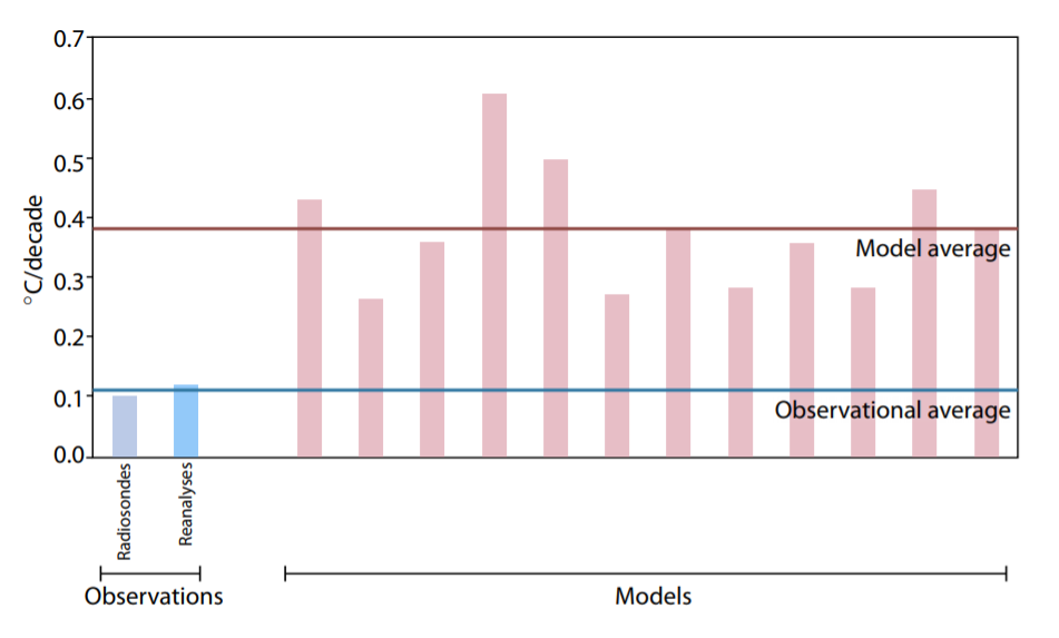
https://rclutz.com/wp-content/uploads/2019/05/christy-2019-fig8.png
Figure 8: Warming in the tropical troposphere according to the CMIP6 models.
Trends 1979–2014 (except the rightmost model, which is to 2007), for 20°N–20°S, 300–200 hPa.
Christy’s comment: We are just starting to see the first of the next generation of climate models, known as CMIP6. These will be the basis of the IPCC assessment report, and of climate and energy policy for the next 10 years. Unfortunately, as Figure 8 shows, they don’t seem to be getting any better. The observations are in blue on the left. The CMIP6 models, in pink, are also warming faster than the real world. They actually have a higher sensitivity than the CMIP5 models; in other words, they’re apparently getting worse! This is a big problem.
Why CMIP6 Models Are More Sensitive
Zelinka et al. (2019) delve into the issue by comparing attributes of the CMIP6 models currently available for diagnostics.
1 Introduction
Determining the sensitivity of Earth’s climate to changes in atmospheric carbon dioxide (CO2) is a fundamental goal of climate science. A typical approach for doing so is to consider the planetary energy balance at the top of the atmosphere (TOA), represented as

where  is the net TOA radiative flux anomaly,
 is the radiative forcing,
 is the radiative feedback parameter, and
 is the global mean surface air temperature anomaly.
The sign convention is that  is positive down and
  is negative for a stable system.
Conceptually, this equation states that the TOA energy imbalance can be expressed as the sum of the radiative forcing and the radiative response of the system to a global surface temperature anomaly. The assumption that the radiative damping can be expressed as a product of a time‐invariant and global mean surface temperature anomaly is useful but imperfect (Armour et al., 2013; Ceppi & Gregory, 2019). Under this assumption, one can estimate the effective climate sensitivity (ECS), the ultimate global surface temperature change that would restore TOA energy balance.

where  is the radiative forcing due to doubled CO
  . .
. .
ECS therefore depends on the magnitude of the CO2 radiative forcing and on how strongly the climate system radiatively damps planetary warming. A climate system that more effectively radiates thermal energy to space or more strongly reflects sunlight back to space as it warms (larger magnitude ) will require less warming to restore planetary energy balance in response to a positive radiative forcing, and vice versa.
Because GCMs attempt to represent all relevant processes governing Earth’s response to CO2, they provide the most direct means of estimating ECS. ECS values diagnosed from CO2 quadrupling experiments performed in fully coupled GCMs as part of the fifth phase of the Coupled Model Intercomparison Project ranged from 2.1 to 4.7 K. It is already known that several models taking part in CMIP6 have values of ECS exceeding the upper limit of this range. These include CanESM5.0.3 , CESM2, CNRM‐CM6‐1, E3SMv1, and both HadGEM3‐GC3.1 and UKESM1.
In all of these models, high ECS values are at least partly attributed to larger cloud feedbacks than their predecessors.
In this study, we diagnose the forcings, feedbacks, and ECS values in all available CMIP6 models. We assess in each model the individual components that make up the climate feedback parameter and quantify the contributors to intermodel differences in ECS. We also compare these results with those from CMIP5 to determine whether the multimodel mean or spread in ECS, feedbacks, and forcings have changed.
The range of ECS values across models has widened in CMIP6, particularly on the high end, and now includes nine models with values exceeding the CMIP5 maximum (Figure 1a). Specifically, the range has increased from 2.1–4.7 K in CMIP5 to 1.8–5.6 K in CMIP6, and the intermodel variance has significantly increased (p = 0.04).
One model’s ECS is below the CMIP5 minimum (INM‐CM4‐8).
This increased population of high ECS models has caused the multimodel mean ECS to increase from 3.3 K in CMIP5 to 3.9 K in CMIP6. Though substantial, this increase is not statistically significant (p = 0.16). ERF  has increased slightly on average in CMIP6 and its intermodel standard deviation has been reduced by nearly 30% from 0.50 Wm^2 in CMIP5 to 0.36 Wm^2 in CMIP6 (Figure 1b).
This ECS increase is primarily attributable to an increased multimodel mean feedback parameter due to strengthened positive cloud feedbacks, as all noncloud feedbacks are essentially unchanged on average in CMIP6. However, it is the unique combination of weak overall negative feedback and moderate radiative forcing that allows several CMIP6 models to achieve high ECS values beyond the CMIP5 range.
The increase in cloud feedback arises solely from the strengthened SW low cloud component, while the non‐low cloud feedback has slightly decreased. The SW low cloud feedback is larger on average in CMIP6 due to larger reductions in low cloud cover and weaker increases in cloud liquid water path with warming. Both of these changes are much more dramatic in the extratropics, such that the CMIP6 mean low cloud amount feedback is now stronger in the extratropics than in the tropics, and the fraction of multimodel mean ECS attributable to extratropical cloud feedback has roughly tripled.
The aforementioned increase in CMIP6 mean cloud feedback is related to changes in model representation of clouds. Specifically, both low cloud cover and water content increase less dramatically with SST in the middle latitudes as estimated from unforced climate variability in CMIP6.

Figure 1. INM-CM5 representation of temperature history. The 5-year mean GMST (K) anomaly with respect to 1850–1899 for HadCRUTv4 (thick solid black); model mean (thick solid red). Dashed thin lines represent data from individual model runs: 1 – purple, 2 – dark blue, 3 – blue, 4 – green, 5 – yellow, 6 – orange, 7 – magenta. In this and the next figures numbers on the time axis indicate the first year of the 5-year mean
The Nitty Gritty

Open image in new tab to enlarge.
The details are shown in Supporting Information for “Causes of higher climate
sensitivity in CMIP6 models”. Here we can seen how specific models stack up on the key variables driving ECS attributes.

Open image in new tab to enlarge.
Figure S1. Gregory plots showing global and annual mean TOA net radiation anomalies
plotted against global and annual mean surface air temperature anomalies. Best-fit ordinary linear least squares lines are shown. The y-intercept of the line (divided by 2) provides an estimate of the effective radiative forcing from CO2 doubling (ERF2x), the slope of the line provides an estimate of the net climate feedback parameter (λ), and the x-intercept of the line (divided by 2) provides an estimate of the effective climate sensitivity (ECS). These values are printed in each panel. Models are ordered by ECS.

Open image in new tab to enlarge.
Figure S7. Contributions of forcing and feedbacks to ECS in each model and for the multimodel means. Contributions from the tropical and extratropical portion of the feedback are shown in light and dark shading, respectively. Black dots indicate the ECS in each model, while upward and downward pointing triangles indicate contributions from non-cloud and cloud feedbacks, respectively. Numbers printed next to the multi-model mean bars indicate the cumulative sum of each plotted component. Numerical values are not printed next to residual, extratropical forcing, and tropical albedo terms for clarity. Models within each collection are ordered by ECS.

Open image in new tab to enlarge.
Figure S8. Cloud feedbacks due to low and non-low clouds in the (light shading) tropics and (dark shading) extratropics in each model and for the multi-model means. Non-low cloud feedbacks are separated into LW and SW components, and SW low cloud feedbacks are separated into amount and scattering components. “Others” represents the sum of LW low cloud feedbacks and the small difference between kernel- and APRP-derived SW low cloud feedback. Insufficient diagnostics are available to compute SW cloud amount and scattering feedbacks for the FGOALSg2 and CAMS-CSM1-0 models. Black dots indicate the global mean net cloud feedback in each model, while upward and downward pointing triangles indicate total contributions from non-low and low clouds, respectively. Models within each collection are ordered by global mean net cloud feedback.
My Summary
Once again the Good Model INM-CM4-8 is bucking the model builders’ consensus. The new revised INM model has a reduced ECS and it flipped its cloud feedback from positive to negative.The description of improvements made to the INM modules includes how clouds are handled:
One of the few notable changes is the new parameterization of clouds and large-scale condensation. In the INMCM5 cloud area and cloud water are computed prognostically according to Tiedtke (1993). That includes the formation of large-scale cloudiness as well as the formation of clouds in the atmospheric boundary layer and clouds of deep convection. Decrease of cloudiness due to mixing with unsaturated environment and precipitation formation are also taken into account. Evaporation of precipitation is implemented according to Kessler (1969).
Cloud radiation forcing (CRF) at the top of the atmosphere is one of the most important climate model characteristics, as errors in CRF frequently lead to an incorrect surface temperature.
In the high latitudes model errors in shortwave CRF are small. The model underestimates longwave CRF in the subtropics but overestimates it in the high latitudes. Errors in longwave CRF in the tropics tend to partially compensate errors in shortwave CRF. Both errors have positive sign near 60S leading to warm bias in the surface temperature here. As a result, we have some underestimation of the net CRF absolute value at almost all latitudes except the tropics. Additional experiments with tuned conversion of cloud water (ice) to precipitation (for upper cloudiness) showed that model bias in the net CRF could be reduced, but that the RMS bias for the surface temperature will increase in this case.
Resources:
Temperatures According to Climate Models Initial Discovery of the Good Model INM-CM4 within CMIP5
Latest Results from First-Class Climate Model INMCM5 The new version improvements and historical validation
Reblogged this on Climate Collections.