Mid October 2023 Arctic Ice Recovering Rapidly


The animation shows Arctic ice rapidly growing from September 30 to yesterday October 16.  Despite much ado about September minimums, in fact the ice recovers quickly from its annual low extent.  Several days exceeded the 17 year average with yesterday slightly in deficit. The graph below shows the distribution of ice across the Arctic Regions with 2023 compare to average, to some notable years and to estimates from SII (Sea Ice Index)

Note that refreezing starts mid September and accelerates upward.  October has already added 1.4M km2 and will likely end up 3M higher than end of September. As the table below shows, the ice extents are tracking the 17 year average and 600k km2 greater than 2007.

Region 2023289 Day 289 2023-Ave. 2007289 2023-2007
 (0) Northern_Hemisphere 6291575 6397434  -105859  5685365 606210 
 (1) Beaufort_Sea 545048 740358  -195309  815519 -270471 
 (2) Chukchi_Sea 399345 309528  89817  98615 300730 
 (3) East_Siberian_Sea 495351 569412  -74061  32547 462804 
 (4) Laptev_Sea 578928 453308  125620  553919 25009 
 (5) Kara_Sea 178575 148145  30430  170928 7647 
 (6) Barents_Sea 22291 42524  -20233  25377 -3086 
 (7) Greenland_Sea 422335 341130  81206  446006 -23670 
 (8) Baffin_Bay_Gulf_of_St._Lawrence 103295 100033  3262  92878 10416 
 (9) Canadian_Archipelago 362514 583556  -221042  502605 -140091 
 (10) Hudson_Bay 208 10894  -10686  1936 -1729 
 (11) Central_Arctic 3179853 3096957  82896  2943760 236093 

Yesterday the overall extent was ~6.30M km2, ~100k km2 below average (2%).  Deficits were mostly in Beaufort Sea and CAA, offset by surpluses in Chukchi,Laptev, and Greenland seas, along with Central Arctic.

Previous post:  2023 September Arctic Outlook and Results Not Scary

The graph above shows the monthly averages for September Arctic ice extents including 2023 compared to previous years back to 2007.  This year is slightly below the 17 year average of 4.63M km2;  MASIE shows 4.43M and SII shows 4.37.  For comparison the 2007 September values were 4.30M for MASIE and 4.27M for SII.  The predictions below refer to the SII value.

2023: August Report from Sea Ice Prediction Network

The August median forecasted value for pan-Arctic September sea-ice extent is 4.60 million square kilometers with interquartile values of 4.35 and 4.80 million square kilometers, while individual forecasts range from 2.88 to 5.47 million square kilometers. We note that the lowest two forecasts predict a new record September sea-ice extent value (current record is September 2012, with a sea-ice extent of 3.57 million square kilometers), but these forecasts are outliers relative to the other contributions.

These are predictions for the September 2023 monthly average ice extent as reported by NOAA Sea Ice Index (SII). This post provides a look at the 2023 Year To Date (YTD) based on monthly averages comparing MASIE and SII datasets. (17 year average is 2006 to 2022 inclusive).

The graph puts 2023 into recent historical perspective. Note how 2023 was slightly below the 17-year average for the first 5 months, then recovered to match average in May and has maintained or exceeded average through August. September was below average slightly and above 2007. The outlier 2012 provided the highest March maximum as well as the lowest September minimum, coinciding with the Great Arctic Cyclone that year.  2007 began the period with the lowest minimum except for 2012.  SII 2023 was running below MASIE except for May/June and is currently just below MASIE and above 2007 and 2012.


Blinded by Antarctica Reports 2023

Special snow goggles for protection in polar landscapes.

Climate Crisis Central apparently triggered Antarctica for this week’s media alarm blitz.

Antarctic Ice Shelves Suffer Staggering Losses | Weather.com

‘Shrinking with no sign of recovery’: Scientists issue warning on Antarctic ice shelves
YAHOO!News

Scientists count huge melts in many protective Antarctic ice shelves. Trillions of tons of ice lost.
Associated Press

Antarctica’s Shrinking Sea Ice Hits a Record Low, Alarming Scientists Bloomberg

Melting Antarctic Ice Shelves Have Dumped More Than 7 Trillion Metric Tons of Water Into the Ocean  The Messenger

Etc., Etc. Etc.

Looks like it’s time yet again to play Climate Whack-A-Mole.  That means stepping back to get some perspective on the reports and the interpretations applied by those invested in alarmism.

Antarctic Basics

The Antarctic Ice Sheet extends almost 14 million square kilometers (5.4 million square miles), roughly the area of the contiguous United States and Mexico combined. The Antarctic Ice Sheet contains 30 million cubic kilometers (7.2 million cubic miles) of ice. (Source: NSIDC: Quick Facts Ice Sheets)

Highly active volcano Mt. Erebus, Ross Island, Antarctica

The Antarctic Ice Sheet covers an area larger than the U.S. and Mexico combined. This photo shows Mt. Erebus rising above the ice-covered continent. Credit: Ted Scambos & Rob Bauer, NSIDC

The study of ice sheet mass balance underwent two major advances, one during the early 1990s, and again early in the 2000s. At the beginning of the 1990s, scientists were unsure of the sign (positive or negative) of the mass balance of Greenland or Antarctica, and knew only that it could not be changing rapidly relative to the size of the ice sheet.

Advances in glacier ice flow mapping using repeat satellite images, and later using interferometric synthetic aperture radar SAR methods, facilitated the mass budget approach, although this still requires an estimate of snow input and a cross-section of the glacier as it flows out from the continent and becomes floating ice. Satellite radar altimetry mapping and change detection, developed in the early to mid-1990s allowed the research community to finally extract reliable quantitative information regarding the overall growth or reduction of the volume of the ice sheets.

By 2002, publications were able to report that both large ice sheets were losing mass (Rignot and Thomas 2002). Then in 2003 the launch of two new satellites, ICESat and GRACE, led to vast improvements in one of the methods for mass balance determination, volume change, and introduced the ability to conduct gravimetric measurements of ice sheet mass over time. The gravimetric method helped to resolve remaining questions about how and where the ice sheets were losing mass. With this third method, and with continued evolution of mass budget and geodetic methods it was shown that the ice sheets were in fact losing mass at an accelerating rate by the end of the 2000s (Veliconga 2009, Rignot et al. 2011b).

Fig. 1. Antarctic Ice Sheet Regions and Drainage Systems (DS). East Antarctica (EA) is divided into EA1 (DS2 to DS11) and EA2 (DS12 to DS17). The Antarctic Peninsula (AP) includes DS24 – 27. West Antarctica (WA) is divided into WA1 (Pine Island Glacier DS22, Thwaites and Smith Glaciers DS21, and the coastal DS20) and WA2 (inland DS1, DS18, and DS19 and coastal DS23). Includes grounded ice within ice shelves and contiguous islands.

Contradictory Findings

A 2021 paper by H. J. Zwally describes the waxing and waning of the Antarctic ice sheet NASA Study: Excess of Mass Gains of the Antarctic Ice Sheet over Mass Losses during 1992 to 2008 Eliminated by Increasing Dynamic Losses to 2016.  Excerpts in italics with my bolds.

A new NASA study [Antarctic Mass Balance] confirms that an increase in Antarctic snow accumulation [Siegert, 2003] that began 10,000 years ago in East Antarctica (EA) [Fig. 1] was adding enough ice to the continent during 1992 to 2008 to outweigh increased losses from its increasing glacier discharge into the ocean from West Antarctica (WA) as previously reported [2015 JOG paper]. Since most other studies reported that the Antarctic ice sheet was losing mass, those 2015 results on gaining mass were controversial. The new study derives consistent rates of mass changes over 24 years (1992 to 2016) using radar-altimetry data from ESA’s Envisat (2003-10) and gravimetry data from NASA’s GRACE (2003-16), in addition to the prior use of radar-altimetry data from ERS1/2 (1992-2001) of the European Space Agency (ESA) and laser-altimetry from NASA’s ICESat (2003-08).

However, the new study shows that beginning in 2009, the dynamic losses from the outlet glaciers in the WA1 part of WA strongly increased by 119 Gt a-1 (from 95 to 214 Gt a-1), which was further enhanced by an accumulation mass decrease of 39 Gt a-1 in the inland WA2 part of WA. Nevertheless, that total decrease of 158 Gt a-1 was not enough to bring the whole ice sheet into balance (input equals output), because there was a concurrent accumulation mass increase of 107 Gt a-1 in EA for three years (2009-11). While that temporary EA accumulation increase diminished, the loss from WA reduced by 71 Gt a-1 and the total ice sheet came into balance at -12 ± 46 Gt a-1 during 2012-16, thereby eliminating its effect on sea level rise.

Fig. 2. M(t) mass time series for West Antarctica (WA), East Antarctica (EA), Antarctica Peninsula (AP), and the total Antarctic Ice Sheet (AIS) from ICESat (blue) and GRACE (red) using the derived equalizing corrections (dBcor and GIAcor) for sub-glacial changes in volume and mass of the Earth’s fluid mantle.

Fig. 3. ICESat map of dM/dt total rate of mass change for 2003-2008 with adjusted correction for bedrock motion.

“We now have an accurate record of how the mass balance of the Antarctic ice sheet has changed over 24 years and the causes of those changes. Short-term changes for 3 to 8 years have been caused by fluctuations in snowfall and accumulation, but there is no significant trend during 1992 to 2016. Mass losses have increased from the dynamic thinning and faster ice discharge of outlet glaciers in West Antarctic, and the large long-term mass gain in East Antarctica has continued”, said lead author Jay Zwally. “However, our findings and those of others [e.g. Barletta and others, 2018] also include some good signs about the future stability of the West Antarctic ice sheet, about which there has been much concern and predictions of increasing mass loss”.

NASA aerial images record West Antarctica melting ice (2016)

Keeping Things in Perspective

Source: NASA

Such reports often include scary graphs like this one and the reader is usually provided no frame of reference or context to interpret the image. First, the chart is showing cumulative loss of mass arising from an average rate of 100 Gt lost per year since 2002. Many years had gains, including 2002, and the cumulative loss went below zero only in 2006.  Also, various methods of measuring and analyzing give different results, as indicated by the earlier section.

Most important is understanding the fluxes in proportion to the Antarctic Ice Sheet.  Let’s do the math.  Above it was stated Antarctica contains ~30 million cubic kilometers of ice volume.  One km3 of water is 1 billion cubic meters and weighs 1 billion tonnes, or 1 gigatonne.  So Antarctica has about 30,000,000 gigatonnes of ice.  Since ice is slightly less dense than water, the total should be adjusted by 0.92 for an estimate of 27.6 M Gts of ice comprising the Antarctic Ice Sheet.

So in the recent decade, an average year went from 27,600,100 Gt to 27,600,000, according to one analysis.  Other studies range from losing 200 Gt/yr to gaining 100 Gt/yr.

Even if Antarctica lost 200 Gt/yr. for the next 1000 years,
it would only approach 1% of the ice sheet.

If like Al Gore you are concerned about sea level rise, that calculation starts with the ocean area estimated to be 3.618 x 10^8 km2 (361,800,000 km2). To raise that area 1 mm requires 3.618×10^2 km3 or 361.8 km3 water (1 km3 water=1 Gt.) So 200 Gt./yr is about 0.55mm/yr or 6 mm a decade, or 6 cm/century.

By all means let’s pay attention to things changing in our world, but let’s also notice the scale of the reality and not make mountains out of molehills.

Let’s also respect the scientists who study glaciers and their subtle movements over time (“glacial pace”).  Below is an amazing video showing the challenges and the beauty of working on Greenland Glacier.

From Ice Alive: Uncovering the secrets of Earth’s Ice

For more on the Joys of Playing Climate Whack-A-Mole 


October 2023 Arctic Ice Flash Freezing

The animation shows the rapid refreezing of Arctic ice from September 30 to yesterday October 9.  Despite much ado about September minimums, in fact the ice recovers quickly from its annual low extent.  As of yesterday, Day 282, this year has again exceeded the 17 year average.

Previous post:  2023 September Arctic Outlook and Results Not Scary

The graph above shows the monthly averages for September Arctic ice extents including 2023 compared to previous years back to 2007.  This year is slightly below the 17 year average of 4.63M km2;  MASIE shows 4.43M and SII shows 4.37.  For comparison the 2007 September values were 4.30M for MASIE and 4.27M for SII.  The predictions below refer to the SII value.

2023: August Report from Sea Ice Prediction Network

The August median forecasted value for pan-Arctic September sea-ice extent is 4.60 million square kilometers with interquartile values of 4.35 and 4.80 million square kilometers, while individual forecasts range from 2.88 to 5.47 million square kilometers. We note that the lowest two forecasts predict a new record September sea-ice extent value (current record is September 2012, with a sea-ice extent of 3.57 million square kilometers), but these forecasts are outliers relative to the other contributions.

These are predictions for the September 2023 monthly average ice extent as reported by NOAA Sea Ice Index (SII). This post provides a look at the 2023 Year To Date (YTD) based on monthly averages comparing MASIE and SII datasets. (17 year average is 2006 to 2022 inclusive).

The graph puts 2023 into recent historical perspective. Note how 2023 was slightly below the 17-year average for the first 5 months, then recovered to match average in May and has maintained or exceeded average through August. September was below average slightly and above 2007. The outlier 2012 provided the highest March maximum as well as the lowest September minimum, coinciding with the Great Arctic Cyclone that year.  2007 began the period with the lowest minimum except for 2012.  SII 2023 was running below MASIE except for May/June and is currently just below MASIE and above 2007 and 2012.

The table below provides the numbers for comparisons (all are M km2)

Monthly MASIE 2023 SII 2023 MASIE -SII MASIE 2023-17 YR AVE SII 2023-17 YR AVE MASIE 2023-2007
Jan 13.579 13.347 0.232 -0.207 -0.250 -0.183
Feb 14.481 14.177 0.304 -0.207 -0.292 -0.171
Mar 14.655 14.440 0.215 -0.212 -0.248 0.032
Apr 13.979 13.992 -0.013 -0.120 -0.025 0.283
May 11.866 12.159 -0.293 -0.742 -0.492 -0.561
June 11.044 10.963 0.081 0.242 0.099 0.218
July 8.431 8.183 0.248 0.152 0.150 0.439
Aug 5.825 5.561 0.264 -0.062 -0.083 0.241
Sept 4.430 4.371 0.059 -0.285 -0.360 0.132

The first two columns are the 2023 YTD shown by MASIE and SII, with the MASIE surpluses in column three.  Column four shows MASIE 2023 compared to MASIE 17 year average, while column five shows SII 2023 compared to SII 17 year average.  YTD September both MASIE and SII ~300k km2 below average. The last column shows MASIE 2023 holding a September surplus of 132k km2 over 2007.

Summary and Update

The experts involved in SIPN were expecting SII 2023 September to be higher than 2007 and somewhat lower than 2022.  The way it came out MASIE September was 285k km2 below average and 132 above 2007.  The Chart below shows the October ice recovery is well under way, now exceeding the average. 

The table shows Day 282 (October 9) ice extents for NH overall and the regions, comparing 2023 to average and several years.

Region 2023282 Day 282 2023-Ave. 2007282 2023-2007
 (0) Northern_Hemisphere 5663965 5537300  126665  4794178 869787 
 (1) Beaufort_Sea 473472 641789  -168317  639935 -166464 
 (2) Chukchi_Sea 323215 255140  68075  14061 309154 
 (3) East_Siberian_Sea 257832 407159  -149327  35 257797 
 (4) Laptev_Sea 471460 252642  218818  340943 130518 
 (5) Kara_Sea 117555 66310  51245  82407 35148 
 (6) Barents_Sea 29729 22272  7457  12933 16796 
 (7) Greenland_Sea 424861 289801  135061  400747 24115 
 (8) Baffin_Bay_Gulf_of_St._Lawrence 90677 67480  23197  73481 17195 
 (9) Canadian_Archipelago 305206 485343  -180137  424350 -119144 
 (10) Hudson_Bay 104 5030  -4926  4163 -4059 
 (11) Central_Arctic 3167292 3043182  124110  2799828 367464 

On Day 282 Arctic ice was 127k km2 above average and nearly 870k km2 above 2007. The major deficits were in Beaufort, East Siberian seas and Canadian Archipelago.  They were more than offset by surpluses in Laptev, Greenland sea and Central Arctic as well as smaller surpluses elsewhere.  From previous years we can expect that October 2023 will gain more than 3M km2 of ice extent over the ending extent in September.


2023 September Arctic Outlook and Results Not Scary

The graph above shows the monthly averages for September Arctic ice extents including 2023 compared to previous years back to 2007.  This year is slightly below the 17 year average of 4.63M km2;  MASIE shows 4.43M and SII shows 4.37.  For comparison the 2007 September values were 4.30M for MASIE and 4.27M for SII.  The predictions below refer to the SII value.

2023: August Report from Sea Ice Prediction Network

The August median forecasted value for pan-Arctic September sea-ice extent is 4.60 million square kilometers with interquartile values of 4.35 and 4.80 million square kilometers, while individual forecasts range from 2.88 to 5.47 million square kilometers. We note that the lowest two forecasts predict a new record September sea-ice extent value (current record is September 2012, with a sea-ice extent of 3.57 million square kilometers), but these forecasts are outliers relative to the other contributions.

These are predictions for the September 2023 monthly average ice extent as reported by NOAA Sea Ice Index (SII). This post provides a look at the 2023 Year To Date (YTD) based on monthly averages comparing MASIE and SII datasets. (17 year average is 2006 to 2022 inclusive).

The graph puts 2023 into recent historical perspective. Note how 2023 was slightly below the 17-year average for the first 5 months, then recovered to match average in May and has maintained or exceeded average through August. September was below average slightly and above 2007. The outlier 2012 provided the highest March maximum as well as the lowest September minimum, coinciding with the Great Arctic Cyclone that year.  2007 began the period with the lowest minimum except for 2012.  SII 2023 was running below MASIE except for May/June and is currently just below MASIE and above 2007 and 2012.

The table below provides the numbers for comparisons (all are M km2)

Monthly MASIE 2023 SII 2023 MASIE -SII MASIE 2023-17 YR AVE SII 2023-17 YR AVE MASIE 2023-2007
Jan 13.579 13.347 0.232 -0.207 -0.250 -0.183
Feb 14.481 14.177 0.304 -0.207 -0.292 -0.171
Mar 14.655 14.440 0.215 -0.212 -0.248 0.032
Apr 13.979 13.992 -0.013 -0.120 -0.025 0.283
May 11.866 12.159 -0.293 -0.742 -0.492 -0.561
June 11.044 10.963 0.081 0.242 0.099 0.218
July 8.431 8.183 0.248 0.152 0.150 0.439
Aug 5.825 5.561 0.264 -0.062 -0.083 0.241
Sept 4.430 4.371 0.059 -0.285 -0.360 0.132

The first two columns are the 2023 YTD shown by MASIE and SII, with the MASIE surpluses in column three.  Column four shows MASIE 2023 compared to MASIE 17 year average, while column five shows SII 2023 compared to SII 17 year average.  YTD September both MASIE and SII ~300k km2 below average. The last column shows MASIE 2023 holding a September surplus of 132k km2 over 2007.

Summary and Update

The experts involved in SIPN were expecting SII 2023 September to be higher than 2007 and somewhat lower than 2022.  The way it came out MASIE September was 285k km2 below average and 132 above 2007.  The Chart below shows the October ice recovery is well under way, reaching average briefly.

The table shows Day 281 (October 8) ice extents for NH overall and the regions, comparing 2023 to average and several years.

Region 2023281 Day 281 2023-Ave. 2007281 2023-2007
 (0) Northern_Hemisphere 5349225 5448341 -99116 4653544 695681
 (1) Beaufort_Sea 429938 633800 -203862 618242 -188304
 (2) Chukchi_Sea 301437 249878 51559 27562 273875
 (3) East_Siberian_Sea 180747 397106 -216358 311 180436
 (4) Laptev_Sea 423091 235120 187971 302924 120168
 (5) Kara_Sea 97994 54598 43396 22717 75277
 (6) Barents_Sea 15003 21167 -6164 3580 11423
 (7) Greenland_Sea 414298 285893 128405 414576 -278
 (8) Baffin_Bay_Gulf_of_St._Lawrence 74944 64730 10214 71399 3545
 (9) Canadian_Archipelago 266487 468946 -202459 408841 -142354
 (10) Hudson_Bay 744 4166 -3423 1936 -1193
 (11) Central_Arctic 3142582 3031785 110797 2780181 362401

On Day 281 Arctic ice was 100k km2 below average and nearly 700k km2 above 2007. The major deficits were in Beaufort, East Siberian seas and Canadian Archipelago.  Offsetting were surpluses in Laptev, Greenland sea and Central Arctic as well as smaller surpluses elsewhere.  From previous years we can expect that October 2023 will gain more than 3M km2 of ice extent over the ending extent in September.


UAH: Amazing SH Land Air Spike September 2023

The post below updates the UAH record of air temperatures over land and ocean. Each month and year exposed again the growing disconnect between the real world and the Zero Carbon zealots.  It is as though the anti-hydrocarbon band wagon hopes to drown out the data contradicting their justification for the Great Energy Transition.  Yes, there is warming from an El Nino buildup coincidental with North Atlantic warming, but no basis to blame it on CO2.  

As an overview consider how recent rapid cooling  completely overcame the warming from the last 3 El Ninos (1998, 2010 and 2016).  The UAH record shows that the effects of the last one were gone as of April 2021, again in November 2021, and in February and June 2022  At year end 2022 and continuing into 2023 global temp anomaly matched or went lower than average since 1995, an ENSO neutral year. (UAH baseline is now 1991-2020).

For reference I added an overlay of CO2 annual concentrations as measured at Mauna Loa.  While temperatures fluctuated up and down ending flat, CO2 went up steadily by ~60 ppm, a 15% increase.

Furthermore, going back to previous warmings prior to the satellite record shows that the entire rise of 0.8C since 1947 is due to oceanic, not human activity.

gmt-warming-events

The animation is an update of a previous analysis from Dr. Murry Salby.  These graphs use Hadcrut4 and include the 2016 El Nino warming event.  The exhibit shows since 1947 GMT warmed by 0.8 C, from 13.9 to 14.7, as estimated by Hadcrut4.  This resulted from three natural warming events involving ocean cycles. The most recent rise 2013-16 lifted temperatures by 0.2C.  Previously the 1997-98 El Nino produced a plateau increase of 0.4C.  Before that, a rise from 1977-81 added 0.2C to start the warming since 1947.

Importantly, the theory of human-caused global warming asserts that increasing CO2 in the atmosphere changes the baseline and causes systemic warming in our climate.  On the contrary, all of the warming since 1947 was episodic, coming from three brief events associated with oceanic cycles. 

Update August 3, 2021

Chris Schoeneveld has produced a similar graph to the animation above, with a temperature series combining HadCRUT4 and UAH6. H/T WUWT

image-8


mc_wh_gas_web20210423124932

See Also Worst Threat: Greenhouse Gas or Quiet Sun?

September 2023 Update New Summer High Driven by SH Spike 

banner-blog

With apologies to Paul Revere, this post is on the lookout for cooler weather with an eye on both the Land and the Sea.  While you will hear a lot about 2020-21 temperatures matching 2016 as the highest ever, that spin ignores how fast the cooling set in.  The UAH data analyzed below shows that warming from the last El Nino had fully dissipated with chilly temperatures in all regions. After a warming blip in 2022, land and ocean temps dropped again with 2023 starting below the mean since 1995.  Spring and Summer 2023 saw a series of warmings.  Now in September a new summer high resulted from a major upward spike in SH, especially the land temps. 

UAH has updated their tlt (temperatures in lower troposphere) dataset for September 2023. Posts on their reading of ocean air temps this month preceded updated records from HadSST4.  I last posted on SSTs using HadSST4 Ocean Warming Crest August 2023, Solar Coincidence?  This month also has a separate graph of land air temps because the comparisons and contrasts are interesting as we contemplate possible cooling in coming months and years. Sometimes air temps over land diverge from ocean air changes.  For example in September 2023, SH land temps leaped upward almost unbelievably.

In September, as shown later on, Global ocean air reached a slightly higher peak led by SH, but with NH easing down. OTOH  Land air temps rose in all regions, with a SH rising dramatically.   Thus the land + ocean Global UAH temperature is now exceeding the 2016 peak.

Note:  UAH has shifted their baseline from 1981-2010 to 1991-2020 beginning with January 2021.  In the charts below, the trends and fluctuations remain the same but the anomaly values change with the baseline reference shift.

Presently sea surface temperatures (SST) are the best available indicator of heat content gained or lost from earth’s climate system.  Enthalpy is the thermodynamic term for total heat content in a system, and humidity differences in air parcels affect enthalpy.  Measuring water temperature directly avoids distorted impressions from air measurements.  In addition, ocean covers 71% of the planet surface and thus dominates surface temperature estimates.  Eventually we will likely have reliable means of recording water temperatures at depth.

Recently, Dr. Ole Humlum reported from his research that air temperatures lag 2-3 months behind changes in SST.  Thus the cooling oceans now portend cooling land air temperatures to follow.  He also observed that changes in CO2 atmospheric concentrations lag behind SST by 11-12 months.  This latter point is addressed in a previous post Who to Blame for Rising CO2?

After a change in priorities, updates are now exclusive to HadSST4.  For comparison we can also look at lower troposphere temperatures (TLT) from UAHv6 which are now posted for September.  The temperature record is derived from microwave sounding units (MSU) on board satellites like the one pictured above. Recently there was a change in UAH processing of satellite drift corrections, including dropping one platform which can no longer be corrected. The graphs below are taken from the revised and current dataset.

The UAH dataset includes temperature results for air above the oceans, and thus should be most comparable to the SSTs. There is the additional feature that ocean air temps avoid Urban Heat Islands (UHI).  The graph below shows monthly anomalies for ocean air temps since January 2015.

Note 2020 was warmed mainly by a spike in February in all regions, and secondarily by an October spike in NH alone. In 2021, SH and the Tropics both pulled the Global anomaly down to a new low in April. Then SH and Tropics upward spikes, along with NH warming brought Global temps to a peak in October.  That warmth was gone as November 2021 ocean temps plummeted everywhere. After an upward bump 01/2022 temps reversed and plunged downward in June.  After an upward spike in July, ocean air everywhere cooled in August and also in September.   

After sharp cooling everywhere in January 2023, all regions were into negative territory. Note the Tropics matched the lowest value, but since have spiked sharply upward +1.26C, with the largest increases in April to July 2023.  NH also warmed 0.7C in the last 4 months, while SH ocean air rose the same. Global Ocean air September 2023 is now matching 2016, the main difference being the much higher rise in SH anomalies since April.  The strength of the El Nino will determine the latter part of this year.

Land Air Temperatures Tracking Downward in Seesaw Pattern

We sometimes overlook that in climate temperature records, while the oceans are measured directly with SSTs, land temps are measured only indirectly.  The land temperature records at surface stations sample air temps at 2 meters above ground.  UAH gives tlt anomalies for air over land separately from ocean air temps.  The graph updated for September is below.

Here we have fresh evidence of the greater volatility of the Land temperatures, along with extraordinary departures by SH land.  Land temps are dominated by NH with a 2021 spike in January,  then dropping before rising in the summer to peak in October 2021. As with the ocean air temps, all that was erased in November with a sharp cooling everywhere.  After a summer 2022 NH spike, land temps dropped everywhere, and in January, further cooling in SH and Tropics offset by an uptick in NH. 

Remarkably, in 2023, SH land air anomaly shot up 1.5C, from  -0.56C in January to +0.93 in July, then dropped to 0.53 in August.  Now in September SH shot up again to 1.5C.  Tropical land temps are up 1.48 since January and NH Land air temps rose 0.9, mostly since May. The consolidated rise greatly exceeds the upward spikes peaking in  2016.

The Bigger Picture UAH Global Since 1980

The chart shows monthly Global anomalies starting 01/1980 to present.  The average monthly anomaly is -0.06, for this period of more than four decades.  The graph shows the 1998 El Nino after which the mean resumed, and again after the smaller 2010 event. The 2016 El Nino matched 1998 peak and in addition NH after effects lasted longer, followed by the NH warming 2019-20.   An upward bump in 2021 was reversed with temps having returned close to the mean as of 2/2022.  March and April brought warmer Global temps, later reversed.

With the sharp drops in Nov., Dec. and January 2023 temps, there was no increase over 1980. Now in 2023 the buildup to the September peak exceeds the sharp April peak of the El Nino 1998 event. It also surpasses the February peak in 2016.  Where it goes from here, up or down, remains to be seen.

TLTs include mixing above the oceans and probably some influence from nearby more volatile land temps.  Clearly NH and Global land temps have been dropping in a seesaw pattern, nearly 1C lower than the 2016 peak.  Since the ocean has 1000 times the heat capacity as the atmosphere, that cooling is a significant driving force.  TLT measures started the recent cooling later than SSTs from HadSST3, but are now showing the same pattern. Despite the three El Ninos, their warming has not persisted prior to 2023, and without them it would probably have cooled since 1995.  Of course, the future has not yet been written.


Doomsday Climate Talk, Deja Vu

At Quora, Dan Gracia responds to this question: (in italics with my bolds)

Q: Why did people start using the term “climate change”
instead of the previous term “global warming”?

I’m 73 now and I remember on April 22, 1970 carrying the totally green American Flag (stars and stripes but in green) at college in a parade celebrating that first Earth Day. Problem then was that we were causing the earth to slip into an ice age due to the use of fluorocarbons as a propellant in spray cans of all types but the most significant factor was their use in hair spray cans. So it was an “Pending Ice Age Alarm”. Well, of course, that didn’t happen as actual temperatures didn’t sink and actually raised very, very slightly (less than a fraction of a degree over the next 10, or was it 20 years?) .

Then it turned into a “Global Warming Alarm” because there was some evidence of an increase in temperatures, regardless of how minuscule it was. So “Global Warming” is the earliest term most people remember now. Then the warming not only did not fit any of the climate models they were/are basing their alarmist claims on, it stopped warming entirely for about 20-years despite Al Gore’s claims the ice-cap would melt and our coasts would be underwater within 10-years.. And then temperatures sank slightly again.

Figure 1: The measured (symbols on left) and modeled (lines) temperature trends vs. altitude. The Russian model comes closest to the data, and the worst fit is GFDL-CM3, Manabe’s model for which he was awarded a Nobel prize. (Fig. 3 from John R. Christy and Richard T. McNider, DOI:10.1007/s13143-017-0070-z, annotated.)

None of these changes fit any of the computer models that were generating the Alarmist predictions. At that point, instead of trying to find out what variable(s) they were missing, the alarmists finally decided to just call it “climate change”. And now they could blame anything even slightly out of the ordinary as due to climate change. It’s a great catch-all term that you can claim regardless of what the temperatures actually show and also because the global climate is in a almost constant state of change. You’d be a fool to deny climate change because the climate is constantly changing and has been for over 4-billion years now. The trick is proving that human interaction is contributing to it in a meaningful and detrimental way. There are so many more powerful forces at play.

Add to that the fact that the earth was in its most prolific state millions of years ago when the Co2 ratio was much higher. Remember those elementary school science lessons that taught you that plants consume (ingest) Co2 (carbon dioxide) and exhaust O2 (oxygen)? Or perhaps that’s not common knowledge anymore? Plants and trees proliferated because growing conditions were better suited for them.

But regardless of weather getting warmer or colder,
climate alarmists are able to blame it all on climate change.

So it’s a catch-all phrase and anyone can chant it for any reason and claim there is a consensus among scientists that this it is a real threat. Unfortunately included in that “consensus” are medical doctors, dentists, Mechanical Engineers, Electrical Engineers, Biologists, Chemists, etc. – basically anyone who has a Bachelor of Science degree or higher. The thing that is missing is a consensus from climatologists. Many of these Bachelor of Science degrees may deal with some fringe parts of the problem but Climatology is an incredibly detailed with ever-changing data field and none of the others have the depth of knowledge to make an accurate claim of cause and effect with enough data and knowledge to make valid predictions.

Would you want a microbiologist to perform open heart surgery on you? Undeniably a scientific background but certainly not enough knowledge and practice to perform a long and complex surgery. Would you look to a Electrical Engineer for that? Definitely a scientist because he/she has at least a bachelor of science degree, ore perhaps a masters or even a doctorate degree. But would you trust that “Doctor” of engineering to perform open-heart surgery on you. Of course not. They don’t have the specialized education, ability to analyze relevant data, or even determine what data was relevant, let alone the fine motor skills needed to successfully complete open heart surgery.

To further muddy the waters, there’s huge amounts of money being spent on climate change research, and if they reach the conclusion that it is not a main ingredient in climate change, that research money dries up and goes away. So actually reaching a provable conclusion whose computer models can be born out with actual evidence instead of speculation, is working towards the elimination of their jobs. Plus, there’s real money to be made outside of climate research projects and grants. There’s the “Carbon TAX”.

Al Gore was one of if not the earliest proponent for “Carbon Credits”. If an industry or installation was generating too much Carbon Dioxide, they would have to purchase the carbon credits to offset their pollution. Ideally this money would then be spent to further other methods of Co2 control. And of course, you would purchase them from Al Gore’s carbon credits company. So then, if the installation had the credits, they could go ahead and continue polluting. As if Al Gore didn’t get enough money from his climate alarmism over the many years he’s been involved this is a Bonanza for him. And how much of that money is actually spent to improve methods and machinery to reduce the carbon levels? How much goes to the top executives of those companies and the people working for them…?

And of course, government has to get in on this cash cow too. A recent carbon tax was imposed on businesses in Washington state. The carbon tax basically requires companies to buy “greenhouse gas allowances,” sold at auction by Washington state, if they emit more than 25,000 metric tons of carbon dioxide per year. The law took effect on Jan. 1, 2023. The first of 4 “auctions” of “greenhouse gas allowances” raised over $300 million dollars. The remaining 3 auctions for the year are expected to raise at least as much resulting in over $1.2 billion dollars for 2023.

Washington State Senator Ericksen said it best, “This legislation will raise billions of dollars from the people of Washington state. Now, who’s going to pay those billions of dollars? It’s not going to be the oil refineries, it’s not going to be the manufacturers, it’s going to be the people of Washington state who will pay through increased costs for their energy.” Anyone who’s had any experience in business from employee to CEO knows that if a company is to stay in business when their costs increase, they either have to raise their prices or decrease their costs. The first place they go to decrease cost is to chop hours and to let people go. Since it’s an industry-wide expense, they all raise their prices because they all have to do so to stay in business – competition doesn’t have a lot to do with this. If they delay raising their prices, then people lose their jobs instead.

As a result of this carbon tax, energy prices have skyrocketed. Promises were made that it certainly wouldn’t raise the price of gas by more than perhaps 5¢ per gallon because it was a tax on businesses, not a raise in the gas tax. In the first 3-weeks of 2023 it went up 25¢ per gallon and now has exceeded a 50¢ per gallon increase. Pricing of Diesel is even worse. Politicians who have never worked a “real job” for a “real business” don’t have much common sense when it comes to raising taxes.

Energy prices have also risen and continue to rise and since virtually everything moves by truck, that drives up the cost of all goods driving inflation even higher. And of course, now that the government has it, they will never let go of that tax regardless of how it hurts their residents.

So this is a self-perpetuating process originated by well meaning folks
who just didn’t have the knowledge or data to back it up.

Absolutely on that first Earth-day in 1970 everyone was concerned for the earth and wanted to find ways to help make it better. Since then it’s become a self-perpetuating scheme with prediction models that have consistently failed over the last 50-years raising alarms which still can’t be proven.

And people seem to forget that Science is not an absolute. What we believe is true today may be disproven tomorrow. THAT is the scientific method regardless of how many people believe in something. At one time virtually all the people in the world believed the earth is flat and the son revolves around the earth. Folks who disagreed were called heretics and persecuted.

The scientific method requires an proposal of what they believes is a reasonable hypothesis that can be proven or disproven. Then through a series of “repeatable” experiments the hypothesis is proven out and published for peer review. If the technique of proving the hypothesis does not generate the same result, then the hypothesis is not proven. Peer review invites dissent, opposing views, and proof of the ability or inability to reach the same result.

NOTE that peer review means scientists who are the peers of those offering the hypothesis with the ability to repeat the experiments used to prove it. You do not solicit or consider the opinion of a medical doctor to a hypothesis put forward by a climatologist, just as you don’t consider the opinion of a climatologist regarding a surgical procedure for a surgeon. Neither are actual peers in the other field of study. They can have opinions, but they are not “peer review”.

As a result I am far more interested in the opinions and research of Dr. Judith Curry and her true peers, than I am of a screaming media darling.

I’m not particularly fond of people
who fly in private jets to a meeting
where they discuss how to take away
my car and feed me bugs . . . but that’s just me.

CO2 Fluxes Are Not Like Cash Flows

I learned alot from a recent extended discussion at Climate Etc. Causality and Climate responding to a paper Demetris Koutsoyiannis et al. (2023) On Hens, Eggs, Temperatures and CO2: Causal Links in Earth’s Atmosphere.   My previous post on this paper was:

Confirmed: Temperature Drives CO2, not the Reverse

I recommend the discussion thread at climate etc. (on going) as a tutorial for the competing paradigms regarding the CO2 cycle.  I gained clarity from the lead author (a frequent and constructive participant) as well others on the core misunderstanding that has plagued such discussions for decades. Some comments are below in italics with my bolds.

First, note that the paper had a narrowly defined scope:  to demonstrate from available data that changes in atmospheric CO2 lag rather than lead temperature changes.  Because the authors recognized that this finding is contrary to IPCC consensus climate science, appendices were supplied to counter the expected objections crediting human CO2 emissions from hydrocarbons as the main, or sole source of rising CO2 since the Little Ice Age (LIA).  As Koutsoyiannis explained in a summary comment near the end:

Demetris Koutsoyiannis September 29, 2023 at 4:54 pm

I think I have rebutted all the different critiques ON MY PAPERS. I am not going to reply to critiques on any other issues related to the issue of climate. Please make your critiques SPECIFIC, by quoting phrases in my papers that you think are incorrect. And before it, please read the papers.

For example you say:

> And that would be the cause of the CO2 increase in the atmosphere?

If you read the paper you will see that we write (p. 17): *What is the cause of the modern increase in temperature? Apparently, this question is much more difficult to reply to, as we can no longer attribute everything to any single agent. We do not claim to have the answer to this question, whose study is far beyond the article’s scope. Neither do we believe that mainstream climatic theory, which is focused upon human CO2 emissions as the main cause and regards everything else as feedback of the single main cause, can explain what happened on Earth for 4.5 billion years of changing climate.*

We have proposed a necessary condition for causality, which is time precedence of the cause over the effect. I hope you accept that necessary condition, am I wrong? We make our inference based on this necessary condition. Your numbers make no reference of time succession. When you find a way to test whether the direction in time is reversed, that will be great. But for now, all this looks to me an unproven conjecture. I hope you can excuse me that, being a Greek, I have to stick to Aristotelian logic.

You also say:

> While there is an elephant in the room, human emissions that released twice as much CO2 as measured in the atmosphere…

If this is the elephant, what is (copying from our paper, p. 25), *a total global increase in the respiration rate of ΔR = 31.6 Gt C/year. This rate, which is a result of natural processes, is 3.4 times greater than the CO2 emission by fossil fuel combustion (9.4 Gt C /year including cement production)*.

My Comment: The confounding issue in all this was identified as the mistaken analogy treating CO2 fluxes as though they are cash transactions between bank accounts.  Within that notion, a natural source/sink must net out intakes and releases.  Yet as others commented, geobiologists know that both absorption and release can be increasing or can be decreasing.  The source/sinks function dynamically, not statically as assumed by the analogy.

clydehspencer | September 29, 2023 at 3:07 pm | 

“Our knowledge of net global uptake over this period is good to 15%.”

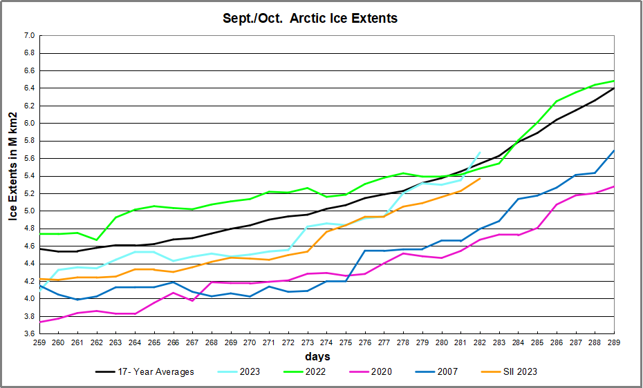
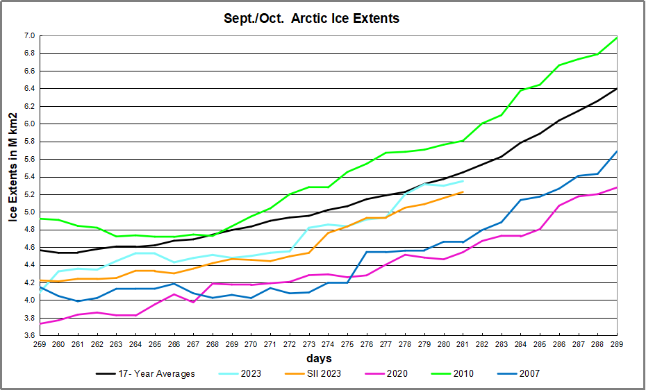
How do you justify making such an assertion when no one has mentioned what is happening in the Arctic, the NASA observation of ‘greening,’ and the utterly unknown situation of submarine volcanic emissions?

How do you propose to identify and dismiss spurious correlations?

Ferdinand Engelbeen | September 29, 2023 at 4:13 pm |

Clyde as said elsewhere, we do not need any natural flow for the carbon balance: that is exactly known from human emissions minus increase in the atmosphere: that is exactly what nature did in the same year: always more sink than source in the past 60 years

Agnostic | October 1, 2023 at 4:23 am |

“In detail: both the oceans and vegetation are proven, increasing (!) sinks for CO2, thus these two can’t be cause of the increase in the atmosphere.
It really is that simple…”

And ironically, this is exactly where you are wrong. Just because they are increasing as sinks does not mean they cannot be increasing as sources. I think you are too stuck on the idea of a “budget”, it’s a linear view. It’s the “net” thing that is where the misunderstanding is.

The biosphere is indifferent to our contribution. If there is more CO2 available it will expand regardless of where it came from. Temperature increase, particularly in winter, means that more CO2 is released in biodegradation than normal. If it releases more than is fixed during the summer growing season, then atmospheric CO2 levels will increase.

During the growing season, if there is more CO2 available, then the biosphere can grow more vigorously and expand. Some of this is semi-permanently fixed, and some will only fix during the growing season to be available to be released as CO2 during the next winter.

If the humans made no contribution, the atmospheric CO2 would still go up, though perhaps not by as much, just as it did in other warm periods during the holocene. This “budget” idea is what is causing the confusion.

Agnostic October 1, 2023 at 4:02 am 

Ferdinand writes: “If humans are not to blame, what is the “other” source (both oceans and vegetation are increasing net sinks) and where resides all that human CO2?”

The same question has to be asked to explain the high variability of CO2 atmospheric concentration prior to industrialisation. The CO2 had to come from somewhere: during the MWP it was as high as 380-390ppm before dropping to 285ppm. During the Bolling-Allerod CO2 increased to as much as 420ppm while temps were actually cooling, a break in the pattern of Temp leading CO2 which holds over all timescales.

The answer is that the biosphere is massively more complex than you are appreciating. You claim that the biosphere is net sink because our emissions are grater than the amount that atmospheric CO2 is rising, but that thinking is too simplistic. It is likely, almost certain given previous periods of warming, that atmospheric CO2 would have risen anyway, but perhaps by not as much, which is our contribution.

The biosphere is expanding because more CO2 is available and is therefore a source as well as a sink. Were we not contributing our share, it would be a net source.

Agnostic | October 1, 2023 at 5:38 am |

“All the variability is in the net sink (not source!) rate of CO2 into nature, while sinks are increasingly negative and temperature is slightly increasing over the same time 60+ years time span…
Thus temperature is NOT the cause of the increase.”

No – this is where you are completely wrong.

The source is ALSO variable. Highly variable. The sinks which you describe as “variable” are ALSO sources, they are interdependent and non-linear in their relationship.

During the growing season, some of the growth fixed via photosynthesis is trapped and some decays during the winter. How much decays is predominantly temperature dependent. The is why you see CO2 follow temperature on ALL timescales that we reliably measure.

Agnostic | October 1, 2023 at 5:33 am | 

Processes that release C into the atmosphere (biodegradation) are far more temperature dependent than processes that fix it (photosynthesis). So there is already a systematic imbalance regardless of anything we do. It is not just a linear “budget”.

During cooler periods, the rate at which CO2 is removed is greater than the rate at which it is released, leading to lowering of CO2 in atmosphere such as LIA. During periods of warmth, especially winter, more CO2 is released than is fixed leading to an increase. But the relationship is not linear.

As more CO2 is available, the transient biosphere expands and grows more vigorously. Some is trapped and some is released at the end of the season. How much is released is dependent on warmth (and to a lesser extent moisture in soils).

We hear the biosphere being described as a “net sink” which is growing because humans emit more C than is remaining in the atmosphere. But it is faulty thinking.

If we did not contribute, then atmosCO2 would still go up, making the biosphere a “net source”. That’s because the biosphere expands and contracts depending on how much CO2 is available and how warm it is. The CO2 comes from trapped sources particularly in the soils, released by increased temperatures which is a much larger overall source than human emissions.

IMO, it is better to think of carbon sources and sinks as dynamic reservoirs that are never perfectly in balance and which have a non-linear relationship with each other. We contribute to the source side, but the biosphere can’t tell the difference between man’s CO2 and naturally emitted, so characterising it as “budget” is where the confusion arises. The “budget” is always changing in non-linear interdependent way. It is not fixed.

Agnostic | October 1, 2023 at 7:59 am |

I have read other similar papers that came to the same conclusion, one in particular by statistician. They were adamant that from a statistical POV you cannot claim causality the way round it is traditionally viewed.

I am NO expert on the carbon cycle, by any means. But it has been bone stuck in my head for a long time because I AM interested in paleoclimatological record. Ice core data is what is generally used to show that CO2 levels are at “unprecedented levels”, yet we know that ice core data is unreliable and too low resolution to speak about short intervals of warming of 300 to 400 years which we appear to be in.

High resolution proxies clearly show similar concentrations of CO2 in the atmosphere
to today, yet that is not put into context. Where did THAT CO2 come from?

The other thing that bothers me is the “budget” approach to CO2 as if there was a fixed amount of C that can be released or absorbed yearly. Yet just the tiniest forays into biodegradation and soil hydrology shows how an incredibly complex and interdependent picture it is, and that’s to say nothing of the oceans.

As usual with climate science, conclusions are made to support a narrative
or a pre-existing conviction and the complexity be damned.

Footnote:  What It Means:  CO2 flows through Dynamic Reservoirs

The other puzzle piece is described by Ed Berry following his peer-reviewed paper Nature Controls the CO2 Increase II.  A summary comment ties his analysis into the above discussion.  Early in the thread the point was made that all CO2 sources are involved in supporting the level of atmospheric concentration at any point in time. Ed Berry made this point  in this way.

He explained that when you look at the flow of carbon dioxide—”flow” meaning the carbon moving from one carbon reservoir to another, i.e., through photosynthesis, the eating of plants, and back out through respiration—a 140 ppm constant level requires a continual inflow of 40 ppm per year of carbon dioxide, because, according to the IPCC, carbon dioxide has a turnover time of 3.5 years (meaning carbon dioxide molecules stay in the atmosphere for about 3 1/2 years).  140 ppm divided by 3.5 is 40 ppm CO2.

“A level of 280 ppm is twice that—80 ppm of inflow. Now, we’re saying that the inflow of human carbon dioxide is one-third of the total. Even IPCC data says, ‘No, human carbon dioxide inflow is about 5 percent to 7 percent of the total carbon dioxide inflow into the atmosphere,’” he said.

[Today’s level of nearly 420 ppm means that 120 ppm of inflow is required annually, or 120 +2 ppm if it is to increase as it has been.  Where does 122 ppm of CO2 come from?  Well, let’s say we can count on 6 ppm of FF CO2 (5%) and  the other 116 being non-human emissions.]

So, to make up for the lack of necessary human-caused carbon dioxide flowing into the atmosphere, the IPCC claims that instead of having a turnover time of 3.5 years, human CO2 stays in the atmosphere for hundreds or even thousands of years.

“The removal of human-emitted CO2 from the atmosphere by natural processes will take a few hundred thousand years (high confidence). Depending on the RCP scenario considered, about 15 to 40% of emitted CO2 will remain in the atmosphere longer than 1,000 years. This very long time required by sinks to remove anthropogenic CO2 makes climate change caused by elevated CO2 irreversible on human time scale.” Source:Chapter 6 Working Group 1 AR5

“[The IPCC is] saying that something is different about human carbon dioxide and that it can’t flow as fast out of the atmosphere as natural carbon dioxide,” Mr. Berry said. “Well, IPCC scientists—when they’ve gone through, what, billions of dollars?—should have asked a simple question:

‘Is a human carbon dioxide molecule exactly identical to a natural
carbon dioxide molecule?’ And the answer is yes. Of course!

“Well, if human and natural CO2 molecules are identical, their outflow times must be identical. So, the whole idea where they say it’s in there for hundreds, or thousands, of years, is wrong.”

Footnote: 

A commenter summed up the discussion this way:

Botanist 

Until a few weeks ago I’d always thought like Ferdinand. This elegant paradigm (below) now seems so simple and obvious, I’m not sure how I did not see it before reading the Hens paper and the article hereabove and contemplating certain helpful comments hereabove. Am I crazy; this strikes me as genius. Can something so simple be.

” My premise is that nature does not make individual balance per source but works holistically. Hence, my version of the carbon balance is roughly this:

Ins: 4% human, 96% natural
Outs: 0% human, 98% natural.
Atmospheric storage difference: +2%
(so that: Ins = Outs + Atmospheric storage difference)

Balance = Atmospheric storage difference: 2%, of which,
Humans: 2% X 4% = 0.08%
Nature: 2% X 96 % = 1.92%
where 1.92% : 0.08% = 24:1 “