Last week Ben Shapiro interviewed Chris Wright concerning the latest moves by realists against the climatists and what’s at stake in this power struggle over humankind’s energy platform, not only for U.S but for the world. For those who prefer reading, I provide a transcript lightly edited from the closed captions, text in italics with my bolds and added images.
Ben: One of the biggest moves that has been made in modern history in the regulatory state has happened this week. The Environmental Protection Agency on Tuesday, according to the Wall Street Journal, declared liberation day from Climate Imperialism by moving to repeal the 2009 so-called endangerment finding for greenhouse gas emissions. So basically, the Clean Air Act, which was put into place in the 1970s, authorized the EPA to regulate pollutants like ozone, particulate matter, sulfur dioxide, and others that might reasonably be anticipated to endanger public health or welfare.
Well, the EPA suggested under Barack Obama that you could use the Clean Air Act in order to regulate carbon emissions, which is insane. That’s totally crazy. The kinds of stuff the Clean Air Act was meant to stop was again particulate matter. It was meant to stop ozone that was breaking down the ozone layer. It was not meant to deal with carbon and particularly carbon dioxide which is a thing that you know is a natural byproduct, for example breathing. Carbon dioxide in the environment is not a danger to human beings.
You may not like what it does in terms of global climate change, but the idea that the EPA has authority under the Clean Air Act is wrong. If Congress wants to give the EPA that authority, then it certainly could, but it never did. The Supreme Court found in 2007 that greenhouse gases could qualify as pollutants under an extraordinarily broad misreading of the law.
But now the EPA is walking that back. And the EPA is suggesting that this is not correct. The Supreme Court and the EPA under their 2009 ruling said, “There is some evidence that elevated carbon dioxide concentrations and climate changes can lead to changes in aeroallergens that could increase the potential for allergenic illnesses.” Well, the Energy Department has now walked that back. They published a comprehensive analysis of climate science and its uncertainties by five outside scientists. One of those is Steven Koonin, who served in the Obama administration.
The crucial point is that CO2 is different from the pollutants Congress expressly authorized the EPA to regulate. Those pollutants are “subject to regulatory control because they cause local problems depending on concentrations including nuisances, damages to plants, and at high enough exposure levels, toxic effects on humans. In contrast, CO2 is odorless, does not affect visibility, and it has no toxicological effects at ambient levels. So, you’re not going to get sick from CO2 in the air.
And so, the EPA administrator Lee Zeldin and Energy Secretary Chris Wright are taking this on. They have said in our interpretation the Clean Air Act no longer applies to greenhouse gases. Well, what does that mean? It means something extraordinary for the American economy, among other things, which is under a massive deregulatory environment.
The alleged cost of regulating greenhouse gas emissions under the Clean Air Act amounts to something like 54 billion per year. So if you multiply that out over the course of the last decade and a half, you’re talking about a cost of in excess of $800 billion based again on a regulatory agency radically exceeding its boundaries.
Well, joining us online to discuss this massive move by the Trump administration is the energy secretary Chris Wright. Secretary, thanks so much for taking the time. Really appreciate it. Thanks for having me, Ben.
Ben: So, first of all, why don’t we discuss what the EPA just did, what that actually means, how’s the energy department involved, and and what does it mean for sort of the future of things like energy developments in the United States?
The Poisonous Tree: Massachusetts v. EPA and the 2009 endangerment finding
Chris: Well, the endangerment finding, 2007 Supreme Court decision, Massachusetts and a bunch of environmental groups sued the EPA and said, “You must regulate greenhouse gas emissions.” Climate activists, basically. Unfortunately the Supreme Court decided five to four in 2007 that greenhouse gases could become endangerments, and if they were the EPA had the option but not the compulsion to regulate greenhouse gases. In 2009, as soon as the Obama administration came in, they did a tortured kind of process to say greenhouse gases endanger the lives of Americans. And that gave the regulatory state, the EPA, the ability to regulate greenhouse gases that the Obama administration and others had failed to pass through Congress. If you pass a law through the House and the Senate and the president signs it, then you can do that. But they just made it up. They just did it through a regulatory backdoor.
And now those those regulations just infuse everything we do, maybe most famously automobiles, the EV mandates, the continual increasing of fuel economy standards that brought us the SUV and everyone buying trucks because they don’t want to buy small cars. But it’s regulating your appliances and power plants and your and home hair dryers and outdoor heaters. So, it’s just been a huge entanglement into American life.
Big brother climate regulations from the government. They don’t do anything meaningful for global greenhouse gas emissions. They don’t change any health outcomes for Americans, but they massively grow the government. They increase costs and they grow the reach of the government. So, Administrator Lee Zeldin is reviewing that and saying, ” We don’t believe that greenhouse gases are a significant endangerment to the American public and they shouldn’t be regulated by the EPA. The EPA does not have authority to regulate them because Congress never passed such a law.
At the Department of Energy, sorry for the long answer, what we did was to reach out to five prestigious climate scientists that are real scientists in my mind; meaning they follow the data wherever it leads, not only if it aligns with their politics or their views otherwise. And we published a long critical overview of climate science and its impact on Americans. And that was released yesterday on the DOE website. I highly recommend everyone to give it a read in synopsis since it’s a big report obviously.
Ben: What are the biggest findings from that report that you commissioned at the Department of Energy with regard to this stuff?
Chris: Maybe the single biggest one that everyone should be aware of is: The ceaseless repeating that climate change is making storms more frequent and more severe and more dangerous is just nonsense. That’s never been in the Intergovernmental Panel on Climate Change (IPCC) reports. It’s just not true.But media and politicians and activists just keep repeating it. And in fact, I saw The Hill had a piece right away when when our press release went out yesterday morning:
Despite decades of data and scientific consensus that climate change is increasing the frequency and intensity of storms, the EPA has reversed the endangerment finding.
Even the headlines are just wrong. One of my goals for 20 years, Ben, is for people to be just a little more knowledgeable of what is actually true with climate change, and what actually are the tradeoffs between trying to reduce greenhouse gas emissions by top- down government actions and what does that mean for the energy system?
We’ve driven up the price of energy, reduced choice to American consumers,
without meaningfully moving global greenhouse gas emissions at all.
And when I talk to activists or politicians about it, they’re not even that concerned about it. They don’t act as if their real goal is to incrementally reduce greenhouse gases in the atmosphere. Their real goal is for the government and them, you know, a small number of people to decide what’s appropriate behavior for all Americans.
Just creepy, top-down control sold in the name of protecting the future of the planet. If it was really about that, they’d know a little bit more about climate change, but they almost never do.
Ben: Well, this is the part that’s always astonishing to me. I get in a room with with climate scientists from places like MIT or Caltech, and we’ll discuss what exactly is going on. These are people who believe that there is anthropogenic climate change, that human activity is causing some sort of market impact on the climate. But when you discuss with them, okay, so what are the solutions? The solutions that that are proposed are never in line with the the kind of risk that they seek to prevent. I mean, the Nobel Prize winning economist William Nordhaus has made the point that there are certain things you could do economically that would totally destroy your economy and might save you an incremental amount of climate change on the other end. And then there are the things that we actually could do that are practical–things like building seawalls, things like hardening an infrastructure, moving toward nuclear energy would be a big one.
And to me, the litmus test of whether somebody is serious or not about climate change is what their feelings are about nuclear energy. If they’re anti-uclear energy, but somehow want to curb climate change, then you know, one of those things is false. It cannot be that you wish to oppose nuclear energy development, also your chief goal is to lower carbon emissions. That’s just a lie.
Chris: Exactly. I mean the biggest driver of reduced greenhouse gas emissions in the US by far has been natural gas displacing coal in the power sector. It’s about 60% of all the US reduction in emissions. But they hate natural gas, you know, because again they’re against hydrocarbons in order to move toward a society that somehow they think is better.
It is helping that more on the left become pro-nuclear. So, I’ll view that as one of the positive side effects of the climate movement and probably is going to help nuclear energy start going again. Of course, there are plenty that are anti-nuclear and climate crazies. So, there’s plenty of them still left. But, as you just mentioned, Nordhaus said in his lecture we should do the things where the benefits are greater than the cost. Sort of common sense. And in his proposed optimal scenario, you know, we reduce the warming through this century by about 20%. Not net zero, because that means you spend hundred trillion dollars and maybe you get $10 trillion of benefits. You know, that’s not good, and then people tell me, well, it’s an admirable goal. It’s aspirational. I’m saying, turning dollars into dimes is not aspirational. It’s human impoverishing.
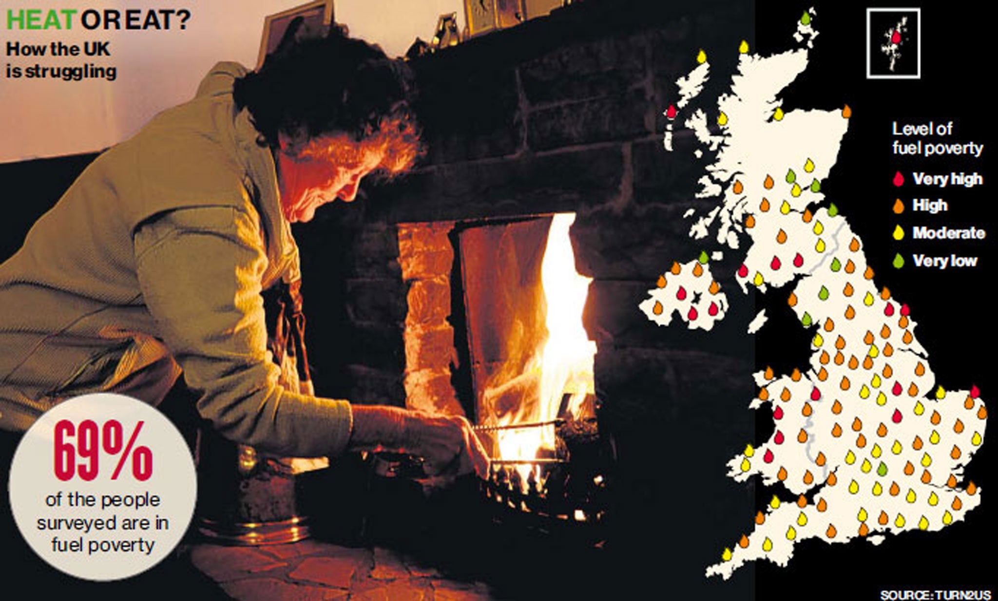
And we can look over to the United Kingdom. They very proudly announced that they have the largest percent reduction in greenhouse gas emissions, 40%. They don’t tell you they’ve had an almost 30% reduction in energy consumption in the United Kingdom. So their dominant mechanism to drive down their greenhouse gas emissions is simply to consume less energy in England. That comes from two factors. The biggest one is their energy intensive industry is shut down in the country and all those jobs have gone overseas.
That stuff is now made in China, loaded on a diesel-powered ship,
shipped back to the United Kingdom, and they call that green.
And the other mechanism is they made energy so expensive that people don’t heat their houses as warm in the winter. They don’t travel as much. They don’t cool their houses as much in the hot summer days. They’ve impoverished their people so they can’t afford needed energy. This isn’t victory and this isn’t changing the global future of the world. We just need back some common sense around energy and climate change.
That’s where the Trump administration is headed across the administration, not just administer Zeldin and myself, but everyone in the administration. We just want Americans to have a government that follows basic common sense.
Ben: Now, Secretary Wright, we were discussing a little bit earlier on in the show this this excellent second quarter GDP number, some of which is being driven certainly by mass investment in technologies like AI. If you talk to folks who are in the capital intensive arenas, pretty much all the money right now is going into AI. That’s a race the United States must win. And one of the huge components there is the energy that is going to be necessary in order to pursue the sorts of processing that AI is going to require. The gigantic data centers that are now being built are going to require inordinate amounts of energy. Everybody knows and acknowledges this. China is producing energy at a rate that far outstrips the United States at this point. So if we wish to actually win the AI race, we have to unleash an all of the above strategy with regard to energy production. That’s obviously something you’re very focused on. And if we don’t win the AI race, in all likelihood China becomes the dominant economic power on planet Earth. So how important is AI to this? And what does it mean for the energy sector?
Chris: It’s massively important. As you just said, it’s what I called it Manhattan Project 2.0. Because in the Manhattan project when we developed an atomic bomb in World War II, we could not have come in second. If Nazi Germany had developed an atomic weapon before us, we would live in a different world now. It’s a similar risk here if China gets a meaningful lead on the US in artificial intelligence.
Because it’s not just economics and science, it’s national defense, it’s the military. Now we are under serious threat from China and we go into a very different world. We must lead in this area. We have the leading scientists. We have businesses. We have the ability to invest these huge amounts of capital again from private markets and private businesses, which a free market capitalist like myself loves.
The biggest limiter as you set up is electricity. The highest form and most expensive type of energy there is turning primary energy into electricity. And as you just said, China’s been growing their electricity production massively. Ours has barely grown in the last 20 years. In fact, it grew like two or 3% in the Obama years, but then during the Biden years, they got prices up over 25%. You could say they helped elect President Trump by just doing everything wrong on energy. And they certainly weren’t into all of the above. They were all about wind, solar, and batteries. And congratulations, they got them to about 3% of total US energy at the end of the Biden years.
The graph shows that global Primary Energy (PE) consumption from all sources has grown continuously over nearly 6 decades. Since 1965 oil, gas and coal (FF, sometimes termed “Thermal”) averaged 88% of PE consumed, ranging from 93% in 1965 to 81% in 2024. Source: Energy Institute
Hydrocarbons went from 82% in 2019, when Biden promised and guaranteed he would end fossil fuels, to 82% his last year in office. Zero change in market share. So they just believe and cling to too many silly things about energy. So today in the United States, the biggest source of electricity by far is natural gas. That will be the dominant growth that will enable us to build all these tens of gigawatts of data centers. It’s abundant, it’s affordable, and it works all the time. I’ve never been an all of the above guy because subsidizing wind and solar is problematic. You know, globally, a few trillions of dollars have gone into it, and if you get high penetration, the main result is expensive electricity and a less stable grid.
That’s not good. The crazy amount of money the United States government spent on wind and solar hasn’t grown our electricity production because they’re not there at peak demand time. Texas has the biggest penetration of wind and second biggest penetration of solar, 35% of the capacity on the Texas grid. But at peak demand with these cold or warm high-pressure systems the wind is gone. Peak demand time is after the sun goes down and you get almost nothing from wind and solar.
Parasites is what they really are. Just in the middle of the day when demand is low, and all the power plants that are needed to supply at peak demand just all have to turn down. And then the sun goes behind a cloud and they got to turn up again. And then when peak demand comes, when it’s very cold at in the evening, all the existing thermal capacity and nuclear capacity has to run and drive the grid.
So if you don’t add to reliable production at peak demand time,
you’re not adding to the capacity of the grid. You’re
just adding to the complexity and cost of the grid.
I mean, if Harris had won the election, we would not only have no chance to win the AI race against China. We would have increasing blackouts and brownouts today, let alone with the the extra demand, some extra demand that would have come from AI, even if they had won the race. But because President Trump won, common sense came back in spades, and we’re allowing American businesses to invest and lead in AI, we’re in a very different trajectory.
Ben: A very different trajectory. Well, that’s US Energy Secretary Chris Wright doing a fantastic job over there. One of the big reasons that the Trump economy continues to churn along. Secretary Wright, really appreciate the time and the insight. Thanks so much for having me, Ben. Appreciate all you do.
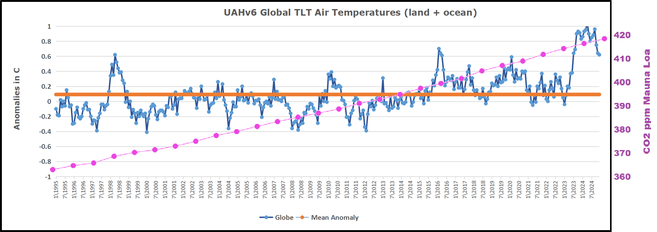
The post below updates the UAH record of air temperatures over land and ocean. Each month and year exposes again the growing disconnect between the real world and the Zero Carbon zealots. It is as though the anti-hydrocarbon band wagon hopes to drown out the data contradicting their justification for the Great Energy Transition. Yes, there was warming from an El Nino buildup coincidental with North Atlantic warming, but no basis to blame it on CO2.
As an overview consider how recent rapid cooling completely overcame the warming from the last 3 El Ninos (1998, 2010 and 2016). The UAH record shows that the effects of the last one were gone as of April 2021, again in November 2021, and in February and June 2022 At year end 2022 and continuing into 2023 global temp anomaly matched or went lower than average since 1995, an ENSO neutral year. (UAH baseline is now 1991-2020). Then there was an usual El Nino warming spike of uncertain cause, unrelated to steadily rising CO2, and now dropping steadily back toward normal values.
For reference I added an overlay of CO2 annual concentrations as measured at Mauna Loa. While temperatures fluctuated up and down ending flat, CO2 went up steadily by ~65 ppm, an 18% increase.
Furthermore, going back to previous warmings prior to the satellite record shows that the entire rise of 0.8C since 1947 is due to oceanic, not human activity.
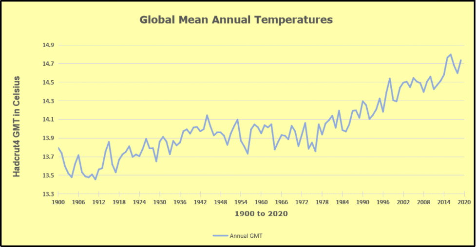
The animation is an update of a previous analysis from Dr. Murry Salby. These graphs use Hadcrut4 and include the 2016 El Nino warming event. The exhibit shows since 1947 GMT warmed by 0.8 C, from 13.9 to 14.7, as estimated by Hadcrut4. This resulted from three natural warming events involving ocean cycles. The most recent rise 2013-16 lifted temperatures by 0.2C. Previously the 1997-98 El Nino produced a plateau increase of 0.4C. Before that, a rise from 1977-81 added 0.2C to start the warming since 1947.
Importantly, the theory of human-caused global warming asserts that increasing CO2 in the atmosphere changes the baseline and causes systemic warming in our climate. On the contrary, all of the warming since 1947 was episodic, coming from three brief events associated with oceanic cycles. And in 2024 we saw an amazing episode with a temperature spike driven by ocean air warming in all regions, along with rising NH land temperatures, now dropping below its peak.
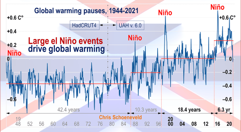
Chris Schoeneveld has produced a similar graph to the animation above, with a temperature series combining HadCRUT4 and UAH6. H/T WUWT
With apologies to Paul Revere, this post is on the lookout for cooler weather with an eye on both the Land and the Sea. While you heard a lot about 2020-21 temperatures matching 2016 as the highest ever, that spin ignores how fast the cooling set in. The UAH data analyzed below shows that warming from the last El Nino had fully dissipated with chilly temperatures in all regions. After a warming blip in 2022, land and ocean temps dropped again with 2023 starting below the mean since 1995. Spring and Summer 2023 saw a series of warmings, continuing into 2024 peaking in April, then cooling off to the present.
UAH has updated their TLT (temperatures in lower troposphere) dataset for July 2025. Due to one satellite drifting more than can be corrected, the dataset has been recalibrated and retitled as version 6.1 Graphs here contain this updated 6.1 data. Posts on their reading of ocean air temps this month are behind the update from HadSST4. I posted recently on SSTs June 2025 Ocean SSTs: NH Warms, SH Cools.These posts have a separate graph of land air temps because the comparisons and contrasts are interesting as we contemplate possible cooling in coming months and years.
Sometimes air temps over land diverge from ocean air changes. In July 2024 all oceans were unchanged except for Tropical warming, while all land regions rose slightly. In August we saw a warming leap in SH land, slight Land cooling elsewhere, a dip in Tropical Ocean temp and slightly elsewhere. September showed a dramatic drop in SH land, overcome by a greater NH land increase. 2025 has shown a sharp contrast between land and sea, first with ocean air temps falling in January recovering in February. Then land air temps, especially NH, dropped in February and recovered in March. Now in July SH ocean dropped markedly, pulling down the Global ocean anomaly despite a rise in the Tropics. SH land also cooled by half, driving Global land temps down despite Tropics land warming.
Note: UAH has shifted their baseline from 1981-2010 to 1991-2020 beginning with January 2021. v6.1 data was recalibrated also starting with 2021. In the charts below, the trends and fluctuations remain the same but the anomaly values changed with the baseline reference shift.
Presently sea surface temperatures (SST) are the best available indicator of heat content gained or lost from earth’s climate system. Enthalpy is the thermodynamic term for total heat content in a system, and humidity differences in air parcels affect enthalpy. Measuring water temperature directly avoids distorted impressions from air measurements. In addition, ocean covers 71% of the planet surface and thus dominates surface temperature estimates. Eventually we will likely have reliable means of recording water temperatures at depth.
Recently, Dr. Ole Humlum reported from his research that air temperatures lag 2-3 months behind changes in SST. Thus cooling oceans portend cooling land air temperatures to follow. He also observed that changes in CO2 atmospheric concentrations lag behind SST by 11-12 months. This latter point is addressed in a previous post Who to Blame for Rising CO2?
After a change in priorities, updates are now exclusive to HadSST4. For comparison we can also look at lower troposphere temperatures (TLT) from UAHv6.1 which are now posted for July 2025. The temperature record is derived from microwave sounding units (MSU) on board satellites like the one pictured above. Recently there was a change in UAH processing of satellite drift corrections, including dropping one platform which can no longer be corrected. The graphs below are taken from the revised and current dataset.
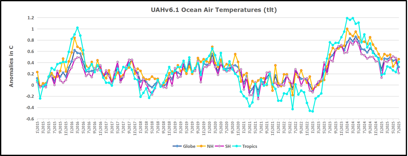
The UAH dataset includes temperature results for air above the oceans, and thus should be most comparable to the SSTs. There is the additional feature that ocean air temps avoid Urban Heat Islands (UHI). The graph below shows monthly anomalies for ocean air temps since January 2015.
In 2021-22, SH and NH showed spikes up and down while the Tropics cooled dramatically, with some ups and downs, but hitting a new low in January 2023. At that point all regions were more or less in negative territory.
After sharp cooling everywhere in January 2023, there was a remarkable spiking of Tropical ocean temps from -0.5C up to + 1.2C in January 2024. The rise was matched by other regions in 2024, such that the Global anomaly peaked at 0.86C in April. Since then all regions have cooled down sharply to a low of 0.27C in January. In February 2025, SH rose from 0.1C to 0.4C pulling the Global ocean air anomaly up to 0.47C, where it stayed in March and April. In May drops in NH and Tropics pulled the air temps over oceans down despite an uptick in SH. At 0.43C, ocean air temps were similar to May 2020, albeit with higher SH anomalies. Now in July Global temps are down to 0.32C due to SH dropping from 0.48C to 0.21C.
Land Air Temperatures Tracking in Seesaw Pattern
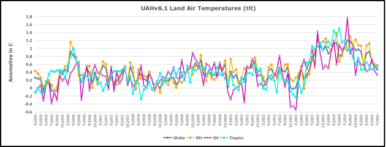
We sometimes overlook that in climate temperature records, while the oceans are measured directly with SSTs, land temps are measured only indirectly. The land temperature records at surface stations sample air temps at 2 meters above ground. UAH gives tlt anomalies for air over land separately from ocean air temps. The graph updated for July is below.
Here we have fresh evidence of the greater volatility of the Land temperatures, along with extraordinary departures by SH land. The seesaw pattern in Land temps is similar to ocean temps 2021-22, except that SH is the outlier, hitting bottom in January 2023. Then exceptionally SH goes from -0.6C up to 1.4C in September 2023 and 1.8C in August 2024, with a large drop in between. In November, SH and the Tropics pulled the Global Land anomaly further down despite a bump in NH land temps. February showed a sharp drop in NH land air temps from 1.07C down to 0.56C, pulling the Global land anomaly downward from 0.9C to 0.6C. In March that drop reversed with both NH and Global land back to January values, holding there in April. In May sharp drops in NH and Tropics land air temps pulled the Global land air temps back down close to February value. In July SH land dropped sharply, down from 0.47C to 0.23C, and NH land also cooled by 0.08C pulling Global land air down as well.
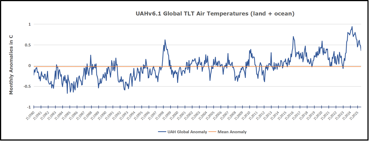
The Bigger Picture UAH Global Since 1980
The chart shows monthly Global Land and Ocean anomalies starting 01/1980 to present. The average monthly anomaly is -0.03, for this period of more than four decades. The graph shows the 1998 El Nino after which the mean resumed, and again after the smaller 2010 event. The 2016 El Nino matched 1998 peak and in addition NH after effects lasted longer, followed by the NH warming 2019-20. An upward bump in 2021 was reversed with temps having returned close to the mean as of 2/2022. March and April brought warmer Global temps, later reversed
With the sharp drops in Nov., Dec. and January 2023 temps, there was no increase over 1980. Then in 2023 the buildup to the October/November peak exceeded the sharp April peak of the El Nino 1998 event. It also surpassed the February peak in 2016. In 2024 March and April took the Global anomaly to a new peak of 0.94C. The cool down started with May dropping to 0.9C, and in June a further decline to 0.8C. October went down to 0.7C, November and December dropped to 0.6C. Now in July Global Land and Ocean is down to 0.36C
The graph reminds of another chart showing the abrupt ejection of humid air from Hunga Tonga eruption.
TLTs include mixing above the oceans and probably some influence from nearby more volatile land temps. Clearly NH and Global land temps have been dropping in a seesaw pattern, nearly 1C lower than the 2016 peak. Since the ocean has 1000 times the heat capacity as the atmosphere, that cooling is a significant driving force. TLT measures started the recent cooling later than SSTs from HadSST4, but are now showing the same pattern. Despite the three El Ninos, their warming had not persisted prior to 2023, and without them it would probably have cooled since 1995. Of course, the future has not yet been written.
Physicist Donald Rapp retired from the Jet Propulsion Laboratory and has authored many books including Ice Ages and Interglacials: Measurements, Interpretation and Models; Assessing Climate Change: Temperatures, Solar Radiation and Heat Balance; and Use of Extraterrestrial Resources for Human Space Missions to Moon or Mars (Astronautical Engineering). Most recently he published Revisiting 2,000 Years of Climate Change (Bad Science and the “Hockey Stick”)
Abstract
The widespread explanations of the greenhouse effect taught to millions of schoolchildren are misleading. The objective of this work is to clarify how increasing CO2 produces warming in current times. It is found that there are two contexts for the greenhouse gas effect. In one context, the fundamental greenhouse gas effect, one imagines a dry Earth starting with no water or CO2 and adding water and CO2 . This leads to the familiar “thermal blanket” that strongly inhibits IR transmission from the Earth to the atmosphere. The Earth is much warmer with H2 O and CO2 . In the other context, the current greenhouse gas effect, CO2 is added to the current atmosphere. The thermal blanket on IR radiation hardly changes. But the surface loses energy primarily by evaporation and thermals. Increased CO2 in the upper atmosphere carries IR radiation to higher altitudes. The Earth radiates to space at higher altitudes where it is cooler, and the Earth is less able to shed energy. The Earth warms to restore the energy balance. The “thermal blanket” is mainly irrelevant to the current greenhouse gas effect. It is concluded that almost all discussions of the greenhouse effect are based on the fundamental greenhouse gas effect, which is a hypothetical construct, while the current greenhouse gas effect is what is happening now in the real world.
Adding CO2 does not add much to a “thermal blanket” but instead,
drives emission from the Earth to higher, cooler altitudes.
Background
Were it not for the Sun, the Earth would be a frozen hulk in space. The Sun sends a spectrum of irradiance to the Earth, the Earth warms, and the Earth radiates energy out to space. This process continues until the Earth warms enough to radiate about as much energy to space as it receives from the Sun, reaching an approximate steady state. If for some reason, the Earth is unable to radiate all the energy received from the Sun, the Earth will warm until it can radiate all the energy received. It is widely accepted that rising CO2 concentration reduces the ability of the Earth to radiate energy to space. In a dynamic situation where the CO2 concentration is continually increasing with time, the Earth will continuously warm as it tries to “catch up” to the effect of increasing CO2 and reestablish a steady state. It is a conundrum that while it is widely accepted that rising CO2 concentration produces global warming, the exact mechanism by which warming is induced in the current atmosphere by rising CO2 is not widely understood. The concept of a “thermal blanket” imposed by greenhouse gases to warm the Earth has merit in some contexts but is mainly irrelevant to the question of how adding CO2 to the current atmosphere produces warming.
Before attempting to deal with the question of how rising CO2 concentration affects the current Earth’s climate, it is appropriate to first discuss the Earth’s energy budget. The exact values for each energy flow are not important, but the relative values are important to show which processes dominate.
Finally, we provide an explanation of how adding CO2 to the current atmosphere produces global warming in the current atmosphere. The mechanism is not widely known and is likely to be surprising to some. Warming does not occur by increasing the thickness of the thermal blanket but instead occurs by raising the altitude at which the Earth radiates to space.
IR radiation
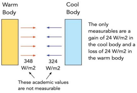
A fundamental law of physics states that all bodies emit a spectrum of radiant power proportional to the fourth power of their absolute temperature. A body at absolute temperature T (K) emits power per unit area: P = σ T 4 = 5.67 x 10 -8 T 4 (W/m 2 ) For example, a body at T = 280 K is said to emit 348 W/m 2 . However, this law of physics is academic and not directly applicable to real-world experience. In the real world, we never have a single isolated body emitting radiation, instead, we deal with pairs of bodies where the warmer one radiates a net flux to the cooler one. (If you stand next to a body at 280 K, you don’t feel an incoming heat flux of 348 W/m 2 ). For example, if there is one body at 280 K and a second body at 275 K, the warmer body will radiate through a vacuum to the cooler body at a net of 24 W/m 2 . That is a real-world parameter that can be measured. But the academic model involves calculating the emission of the warm body as 348 W/m 2 and the emission of the cooler body as 324 W/m 2, and subtracting, the net transfer from the warm body to the cool body is 24 W/m 2 . But the calculated values are academic and cannot be measured in the real world with 348 W/m 2 in one direction and 324 W/m 2 in the opposite direction. Those values are only of academic use to infer the measurable net of about 24 W/m 2 . See the simple model in Figure 1 presented here for illustration.
Figure 1: Radiant heat transfer between warm and cool bodies
The two contexts of the greenhouse effect
We are all aware of the widely discussed greenhouse effectthat warms the Earth as the concentration of greenhouse gases increases. But just how does it work?Here, we define two contexts for greenhouse gas effects:
1) The fundamental greenhouse gas effectcan be described by a “gedanken experiment” in which one imagines a dry Earth starting with no water or CO 2 and begins adding water and CO 2 . The original atmosphere, lacking water and CO 2 , will transmit IR radiation completely. As a result, the Earth will be quite cool. As H 2 O and CO 2 are added to the atmosphere, the transmission of IR radiation from the Earth’s surface is increasingly inhibited, and the Earth warms. As the Earth warms, evaporation and thermals transmit more energy from the Earth to the atmosphere. By the time H 2 O and CO 2levels reach current levels, the atmosphere is almost opaque to IR radiation, and a “thermal blanket” greatly reduces IR transmission from the Earth to the atmosphere. The Earth cools primarily by evaporation and thermals, and it is much warmer than if CO 2 and water were absent. The notion of a “thermal blanket” of IR absorbing gases warming the Earth has validity in this context starting with a transmitting atmosphere and adding greenhouse gases. However, once the thermal blanket is established with ~ 400 ppm CO 2 , adding more CO 2 has only a small effect on reducing IR radiation from the surface.
2) The current greenhouse gas effectdeals with the question: How does the addition of CO 2 to the atmosphere affect the global average temperature in 2024 and beyond, with CO 2 around 400+ ppm? It was shown previously that starting with no water or CO 2 , adding H 2 O and CO 2 to the atmosphere generates a “thermal blanket” for radiation. But once that “thermal blanket” is well established and the lower atmosphere is very opaque to IR radiation, what is the effect of adding even more CO 2 ? Dufresne, et al. provide a detailed technical analysis to show how the current greenhouse effect works [7]. However, this reference is complex and written for expert specialists in IR transmission through the atmosphere. In the sections that follow, a simpler, qualitative interpretation will be presented.
Figure 3: Energy flows in the Earth’s system. (Based on LTWS references).
Energy budget of the earth
Energy transfer in the Earth system can take place by thermal transfers (“thermals”) where winds carry warm air up to colder regions, evaporation from the surface (removes heat), and condensation in the atmosphere (deposits heat) and radiation (further discussion follows).
After analyzing the data in the LTWS references (see Section 1.2), a rough estimate of key energy flows per unit time in the Earth system is given as follows. The exact numbers are not critical; only their relative values are important for this discussion.
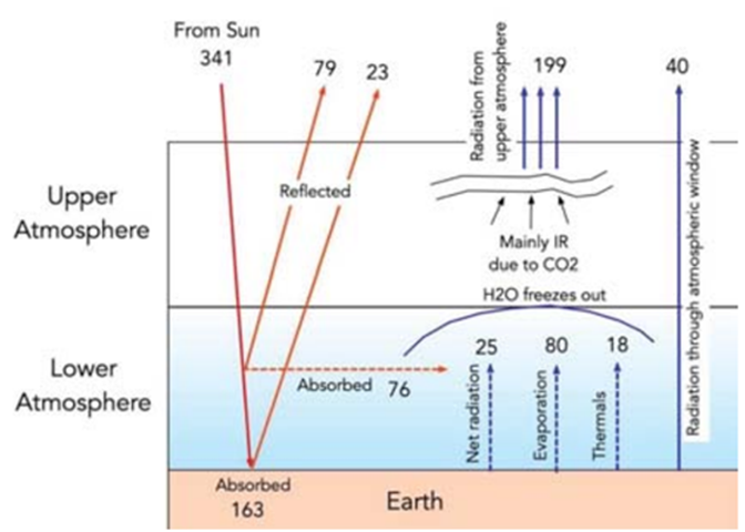
These results can be visualized in Figure 3 which is based on the references LTWS. As shown in Figure 3, incoming solar irradiance (341 W/ m 2 ) is partly reflected by the lower atmosphere back out tospace (79 W/m 2 ), partly reflected by the Earth’s surface back out to space (23 W/m 2 ), partly absorbed by the lower atmosphere (76 W/m 2 ), and finally about 163 W/m 2 is absorbed by the surface.
Radiation from the Earth’s surface to the lower atmosphere requires further discussion. The LTWS references show high up and down radiation flows. For example, Trenberth, et al. did not show radiation transfer between the Earth’s surface as a simple 25 W/m 2 net radiative transfer from the surface to the lower atmosphere. Instead, they showed 356 W/m 2 radiated upward from the surface and 333 W/m 2 of “back radiation” from the atmosphere to the surface [2]. The figure 356 W/m 2 radiated upward from the surface corresponds to the theoretical radiation from a blackbody at 281.5 K. The claimed downward figure is difficult to explain. But both of these figures are academic. What is happening is that the warm Earth is radiating upward through an optically thick gas of H 2 O and CO 2 absorbers, and the radiant transfer through that thick gas is estimated to be only a mere ~25 W/m 2. This is the “thermal blanket” so often referred to in discussions of global warming. The thermal blanket is real. But the problem with so many discussions of the greenhouse effect is that there is a preoccupation with radiant energy transfer between the Earth and the atmosphere (which is “blanketed”) while neglecting the more important transfers of energy to the atmosphere by processes other than radiation.
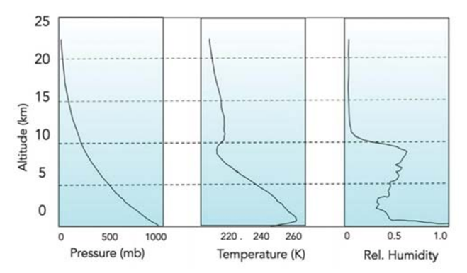
Figure 4: Pressure, temperature, and relative humidity vs. altitude [8].
The terms “lower atmosphere” and “upper atmosphere” are defined next. Following Miscolczi, Figure 4 shows that the demarcation between upper and lower atmospheres occurs at an altitude of roughly 12 km above which H 2 O is frozen out and the temperature roughly stabilizes [8].
Energy transfer in the lower atmosphere takes place by conduction,
convection, and radiation. Energy transfer in the upper atmosphere
takes place primarily by radiation.
The greenhouse effect
The greenhouse effect can only be fully understood by comprehensive modeling of upward energy flows in the Earth system. Excellent studies by Dufresne, et al. and Pierrehumbert provide detailed physics [7,9]. Here, we interpret these results qualitatively.
Within the Earth system of land, ocean, atmosphere, and clouds, energy transfer is taking place continuously. There is a net energy flow upward toward higher altitudes. From the surface of the Earth, much of the upward flow of energy in the lower atmosphere is through evaporation and convection. The lower atmosphere is almost opaque to IR radiation due to water vapor and CO 2.
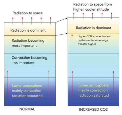
Figure 5: Qualitative sketch to show radiation is dominant at the highest altitude. By adding CO2 to the atmosphere, radiative energy transport is carried to a higher altitude where it is colder, reducing the radiant power emitted by the upper atmosphere.
Radiation energy transfer will persist out toward a high altitude until the CO 2 concentration diminishes. Each CO 2 molecule that absorbs an IR photon can reradiate in all directions, but in a thin atmosphere, some upward IR radiation will be lost, and on a net basis, this allows the Earth to radiate out to space. The presence of an IR transmitting/absorbing gas (CO 2 ) will allow energy transport to higher altitudes. The highest altitude where there is enough thin gas to maintain radiation is the region of the atmosphere that mainly radiates energy outward to space. This is illustrated on the left side of Figure 5. Figure 5 was created here to illustrate how the predominant energy transfer mechanisms gradually change to IR radiation at higher altitudes, and the presence of CO 2 carries the IR radiation to higher altitudes.
Conclusion
There are two different contexts for discussion of the effect of greenhouse gases on the Earth’s climate.
In one context, one can imagine an Earth with no water vapor or CO 2 in the atmosphere. This Earth can radiate effectively to space and is relatively cold. As water vapor and CO 2 are added to the atmosphere, the IR-opacity of the atmosphere increases and the Earth system warms. The greenhouse gases act as a “thermal blanket” to warm the Earth by impeding upward IR radiation. This is labeled the fundamental greenhouse gas effect. However, once the thermal blanket is established, adding more CO 2 has only a minimal effect on the thermal blanket, and reduced upward IR radiation from the surface does not produce significant warming. This is referred to by Dufresne, et al. [7] as the “saturation paradox”.
In the other context, we are concerned with the effect of adding more CO 2 to the current atmosphere where the CO 2 concentration is already 400+ ppm, and the thermal blanket is already in place, restricting upward IR-radiation. This is labeled the current greenhouse gas effect, and it is quite different from the fundamental greenhouse gas effect. In the current atmosphere, energy transfer from the Earth to the atmosphere is primarily by evaporation and thermals, and IR-radiant energy transfer is significantly impeded by an almost opaque lower atmosphere. The “thermal blanket” is in place, but it doesn’t change much as CO 2 is added to the atmosphere. Adding CO 2 to the current atmosphere slightly increases the opacity of the lower atmosphere but this is of little consequence.
In the upper atmosphere, CO 2 is the major means of energy transport by IR radiation. The greatest effect of adding CO 2 to the current atmosphere is to extend the upward range of IR-radiant transmission to higher altitudes. The main region where the Earth radiates to space is thereby extended to higher altitudes where it is colder, and the Earth cannot radiate as effectively as it could with less CO 2in the atmosphere. The Earth warms until the region in the upper atmosphere where the Earth radiates to space is warm enough to balance incoming solar energy.
My Comment:
The explanation above is clear and understandable in qualititative terms. It does not reference empirical evidence regarding a GHG effect from a raised effective radiating level (ERL). Studies investigating this theory find that the effect is too small to appear in the data.
The following diagram by Andy May shows the pattern of emissions by GHGs, mainly H2O and CO2.
Helpfully, it shows the altitudes where the emissions occur. As stated in the text above, the upper and lower tropopsphere shift occurs about 12km high, with variations lower at poles and higher in tropics. Note the large CO2 notch appears at 85km, which puts it into the thermosphere, where temperatures increase with altitude. Raising the ERL there means greater cooling, not less. The Ozone notch at 33km is in the stratosphere, where temperatures also rise with altitude. Otherwise almost all of the IR effect is from H2O.
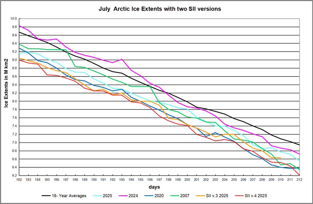
NSDIC acknowledged my query regarding the SII (Sea Ice Index) dataset, which is described below. While awaiting an explanation I have investigated further. My last download of the SII Daily Arctic Ice Extents was on July 30, meaning that the most recent data in that file was day 210, July 29. The header on that file was Sea_Ice_Index_Daily_Extent_G02135_v3. Then on August 1, the downloaded file had the heading Sea_Ice_Index_Daily_Extent_G02135_v4. So it appears that these are now the values from a new version of SII. As I wrote in my query, since March 14 all of the values for Arctic Ice Extents are lower in this new record. The graph below shows the implications for July as an example.
You can see how v.4 in red is lower than v.3 in orange throughout the month. It may be that v.3 values will no longer be reported in the future, though that has not been confirmed to me. It should also be noted that v.3 values for 2024 and prior years have also been altered in v.4 and I intend to look into that impact.
Note: After comparisons of monthly averages, results from the two versions appear comparable for previous years. The change started in January 2025 and will be the basis for future reporting. The logic for this is presented in this document: Sea Ice Index Version 4 Analysis
In June 2025, NSIDC was informed that access to data from the Special Sensor Microwave Imager/Sounder (SSMIS) onboard the Defense Meteorological Satellite Program (DMSP) satellites would end on July 31 (NSIDC, 2025). To prepare for this, we rapidly developed version 4 of the Sea Ice Index. This new version transitions from using sea ice concentration fields derived from SSMIS data as input to using fields derived from the Advanced Microwave Scanning Radiometer 2 (AMSR2) sensor onboard the Global Change Observation Mission – W1 (GCOM-W1) satellite. On 29 July 2025, we learned that the Defense Department decision to terminate access to DMSP data had been reversed and that data will continue to be available until September 2026. We are publishing Version 4, however, for these reasons:
• The SSMIS instruments are well past their designed lifespan and a transition to AMSR2 is inevitable. Unless the sensors fail earlier, the DoD will formally end the program in September 2026. • Although access of SSMIS will continue through September 2026, the Fleet Numerical Meteorology and Oceanography Center (FNMOC), where SSMIS data from the DMSP satellite are downloaded, made an announcement that “Support will be on a best effort basis and should be considered data of opportunity.” This means that SSMIS data will likely contain data gaps. • We have developer time to make this transition now and may not in the future. • We are confident that Version 4 data are commensurate in accuracy to those provided by Version 3.
Overview
Before presenting the MASIE and SII results for July, a note about a strange thing in today’s Sea Ice Index report. I have sent a note to them requesting an explanation for why the values have been altered from those in the dataset just two days ago. When attempting to add into my spreadsheets the final two July days, I noticed that all the previous values were now different. Exploring further, going back to beginning of 2024 all values had changed, some showing larger extents and many showing smaller ice extents than previous recorded.
For 2024 the new values added ice extents with the average day gaining slightly (47k km2). But in 2025 so far, the average day lost (-57k km2) compared to the values two days ago. Curiously, since March 14, 2025 all days had lower values at a daily rate of -75k km2. In sum, the altered values in 2025 removed ~11M km2 of ice extents so far, and 10M km2 of that since March 14. In the report below, I excluded the altered SII values awaiting news from NSIDC.
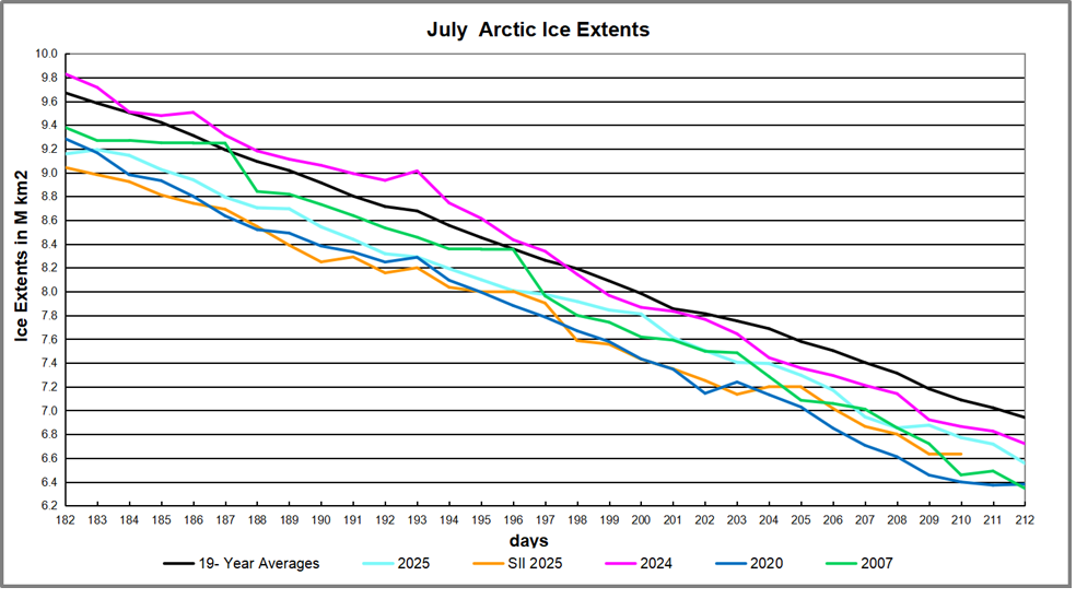
After a sub-par March maximum, by end of May 2025 Arctic ice closed the gap with the 19-year average. Then in June the gap reopened and in July the melting pace matched the average, abeit four days in advance of average. The chart shows the July Arctic ice extents on average decline from 9.7M to 6.9M km2. MASIE started July ~5M km2 in deficit to average and ended the month ~4M km2 down, continuing to melt about four days in advance of the average decline. SII matched MASIE the first half of July, then tracked slightly lower the second half.
The regional distribution of ice extents is shown in the table below. (Bering and Okhotsk seas are excluded since both are now virtually open water.)
Region
2025212
Day 212
2025-Ave.
2020212
2025-2020
(0) Northern_Hemisphere
6555733
6941055
-385322
5880746
674988
(1) Beaufort_Sea
944231
793206
151025
875454
68777
(2) Chukchi_Sea
621236
555019
66217
533748
87488
(3) East_Siberian_Sea
683122
751512
-68390
329453
353669
(4) Laptev_Sea
329581
370847
-41266
61979
267602
(5) Kara_Sea
32436
166826
-134390
95539
-63103
(6) Barents_Sea
1131
29555
-28424
23940
-22808
(7) Greenland_Sea
228078
296681
-68603
282403
-54325
(8) Baffin_Bay_Gulf_of_St._Lawrence
117170
150751
-33581
35368
81801
(9) Canadian_Archipelago
460908
547942
-87034
515499
-54592
(10) Hudson_Bay
73633
139798
-66165
92861
-19228
(11) Central_Arctic
3062678
3137162
-74483
3033706.07
28972
The table shows most regions in deficit with Kara the largest, and Canadian Archipelago and Central Arctic also sizable. Hudson Bay and Greenland Sea will lose the rest of their ice in upcoming weeks. Surpluses in Beaufort and Chukchi offset about 220k km2 of losses elsewhere.
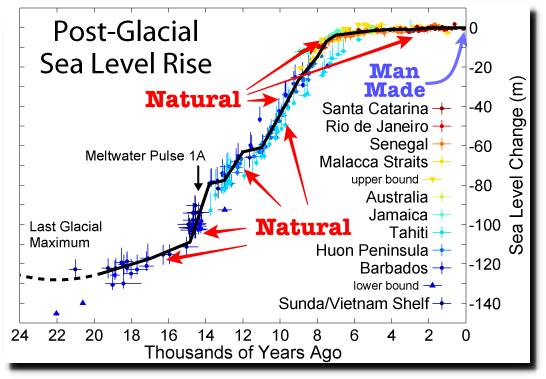
Why is this important? All the claims of global climate emergency depend on dangerously higher temperatures, lower sea ice, and rising sea levels. The lack of additional warming prior to 2023 El Nino is documented in a post NH and Tropics Lead UAH Temps Lower May 2025.
Illustration by Eleanor Lutz shows Earth’s seasonal climate changes. If played in full screen, the four corners present views from top, bottom and sides. It is a visual representation of scientific datasets measuring Arctic ice extents and NH snow cover.
Before presenting the MASIE and SII results for July, a note about a strange thing in today’s Sea Ice Index report. I have sent a note to them requesting an explanation for why the values have been altered from those in the dataset just two days ago. When attempting to add into my spreadsheets the final two July days, I noticed that all the previous values were now different. Exploring further, going back to beginning of 2024 all values had changed, some showing larger extents and many showing smaller ice extents than previous recorded.
For 2024 the new values added ice extents with the average day gaining slightly (47k km2). But in 2025 so far, the average day lost (-57k km2) compared to the values two days ago. Curiously, since March 14, 2025 all days had lower values at a daily rate of -75k km2. In sum, the altered values in 2025 removed ~11M km2 of ice extents so far, and 10M km2 of that since March 14. In the report below, I excluded the altered SII values awaiting news from NSIDC.
After a sub-par March maximum, by end of May 2025 Arctic ice closed the gap with the 19-year average. Then in June the gap reopened and in July the melting pace matched the average, abeit four days in advance of average. The chart shows the July Arctic ice extents on average decline from 9.7M to 6.9M km2. MASIE started July ~5M km2 in deficit to average and ended the month ~4M km2 down, continuing to melt about four days in advance of the average decline. SII matched MASIE the first half of July, then tracked slightly lower the second half.
The regional distribution of ice extents is shown in the table below. (Bering and Okhotsk seas are excluded since both are now virtually open water.)
Region
2025212
Day 212
2025-Ave.
2020212
2025-2020
(0) Northern_Hemisphere
6555733
6941055
-385322
5880746
674988
(1) Beaufort_Sea
944231
793206
151025
875454
68777
(2) Chukchi_Sea
621236
555019
66217
533748
87488
(3) East_Siberian_Sea
683122
751512
-68390
329453
353669
(4) Laptev_Sea
329581
370847
-41266
61979
267602
(5) Kara_Sea
32436
166826
-134390
95539
-63103
(6) Barents_Sea
1131
29555
-28424
23940
-22808
(7) Greenland_Sea
228078
296681
-68603
282403
-54325
(8) Baffin_Bay_Gulf_of_St._Lawrence
117170
150751
-33581
35368
81801
(9) Canadian_Archipelago
460908
547942
-87034
515499
-54592
(10) Hudson_Bay
73633
139798
-66165
92861
-19228
(11) Central_Arctic
3062678
3137162
-74483
3033706.07
28972
The table shows most regions in deficit with Kara the largest, and Canadian Archipelago and Central Arctic also sizable. Hudson Bay and Greenland Sea will lose the rest of their ice in upcoming weeks. Surpluses in Beaufort and Chukchi offset about 220k km2 of losses elsewhere.
Why is this important? All the claims of global climate emergency depend on dangerously higher temperatures, lower sea ice, and rising sea levels. The lack of additional warming prior to 2023 El Nino is documented in a post NH and Tropics Lead UAH Temps Lower May 2025.
Illustration by Eleanor Lutz shows Earth’s seasonal climate changes. If played in full screen, the four corners present views from top, bottom and sides. It is a visual representation of scientific datasets measuring Arctic ice extents and NH snow cover.