How Sun and Cosmic Rays Make Our Climate Change


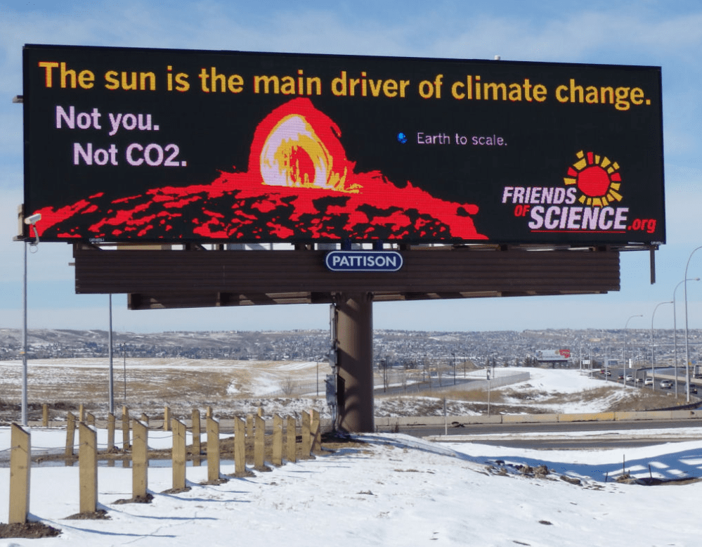
Dr. Henrik Svensmark: Sun and Cosmic Rays Drive Climate, Not CO₂

Danish astrophysicist Henrik Svensmark explains how the changes in solar activity and cosmic rays can influence cloud formation and therefore our climate on Earth. Title above is link to podcast video at Freedom Research.  Below is the transcript lightly edited with my bolds and added images. FR refers to Freedom Research interviewer Hannes Sarv, and HS refers to Henrik Svensmark.

Hello, welcome. This is the Freedom Research Podcast and my name is Hannes Sarv. My guest today is a researcher from Denmark, an astrophysicist, Henrik Svensmark. He’s well known for his research on the relationship between cosmic rays and Earth’s climate. He has proposed that the variations in cosmic radiation influence cloud formation and consequently global temperature and biodiversity. Of course, we’re going to talk about climate change, cosmic rays and supernovas and how they affect Earth’s climate and biodiversity well here on Earth. So first of all, thank you, Henrik, for taking the time for this interview.

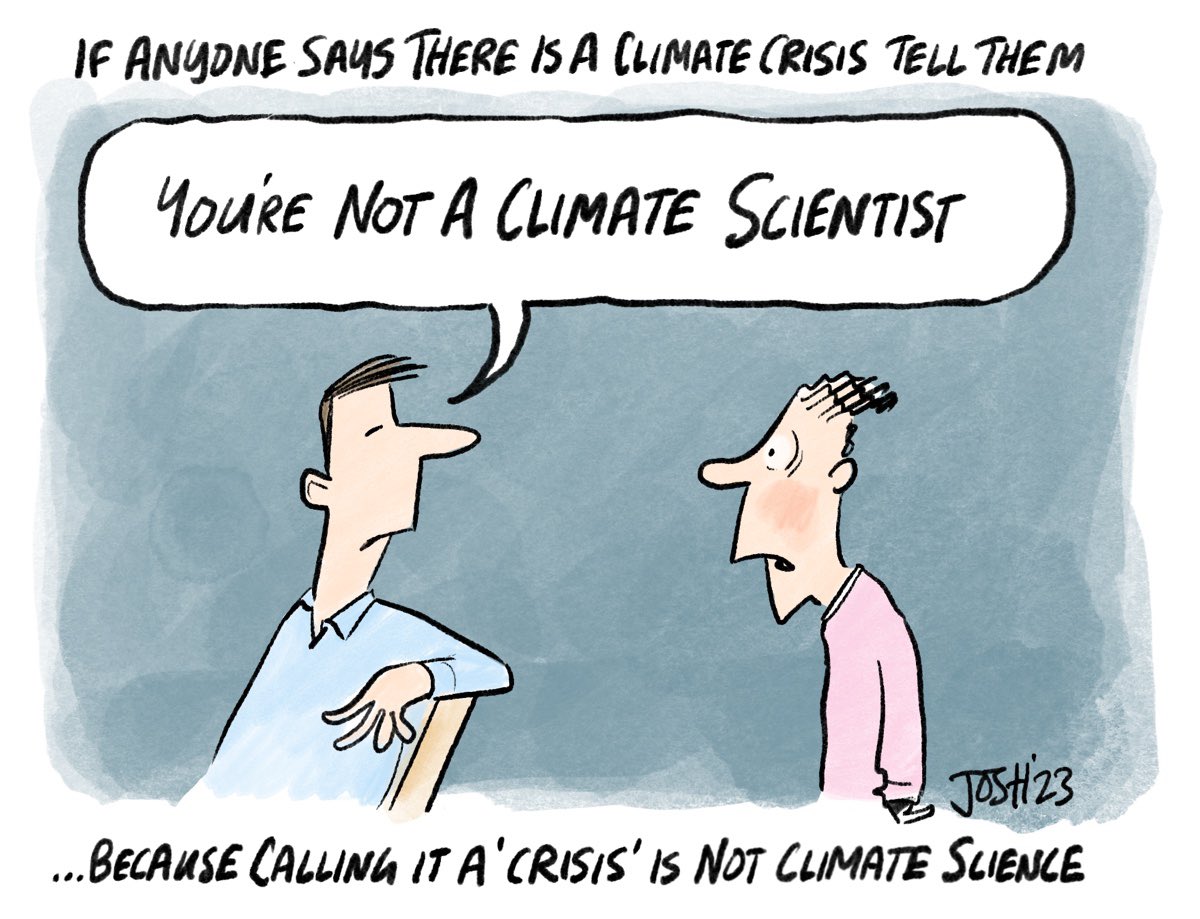
Firstly, I would actually like to ask a question. Simple, simple question, which can be puzzling, at least to a lot of people. I mean, if you’re being told that you’re living in a constant climate crisis, then probably most of the people probably fear it or they might get afraid. So if someone says to you that today there is a climate crisis. What is your answer to that?

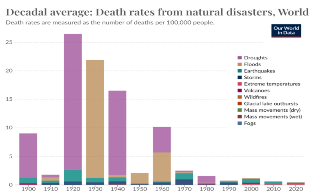
HS: Well, it’s a very political subject and the idea that the climate is in a crisis, I don’t think that that’s actually the case. It’s much less I mean, the climate disasters and so on, I mean, they’re not really increasing at all. And, of course, the temperature has gone up a little bit, but it has not, you know, made a serious crisis that we cannot handle. So, I actually think the idea that we are in a crisis is actually not correct.
FR: So you think, probably It depends on where you live, right? If the temperature goes up, it gets warmer and well, as I have understood most of the places or the larger part of the population actually benefits from higher temperatures.  What is your take?

HS: Certainly, there are places where you actually benefit from it. And in many cases, it’s not because it actually gets warmer. It’s more like it’s climate’s getting milder, meaning that it’s the colder temperatures, you know, at night and in the winter that goes slightly up, which is actually a good thing.  I mean, here in Denmark, we haven’t had very severe winters for a long time. which is also good. It’s good for the economy. It’s good for many things because a cold climate is much, much worse than a warmer climate. I think that, I mean, you also know that You also talk about people, you can have people dying from warm weather, but we know that it’s mainly cold weather that is the real killer of people. I think there’s almost a factor of 10 in difference. So slightly milder weather is not a problem. I mean, it’s certainly not a disaster.
FR:This is kind of puzzling also to many people, if they’re being told that the planet is going to be inhabitable.  Then there’s talk of sea level rise and all those other apocalyptic things that make good movies. But the actual truth there is at least a bit more complex, would you say?

HS: Yes, there’s been so many claims. I think also people should get tired of all the predictions that are wrong. I mean, that there would be no ice in the Arctic and Greenland is melting and so on. And, you know, the islands in the Pacific should be subsiding because of the rising sea levels.  And it’s not really happening, any of these things. And all these predictions, which I mean, it gets everybody’s attention, of course, because we are sort of prone to react when we hear about disasters, or coming disasters. They are not really happening fortunately. I mean, it’s actually a good thing that it’s actually not occurring.

FR: So when we look at a longer time frame, it should be brought out that there have been many such crises that have threatened all life and human life. So can you just maybe make a comparison here to today’s climate?

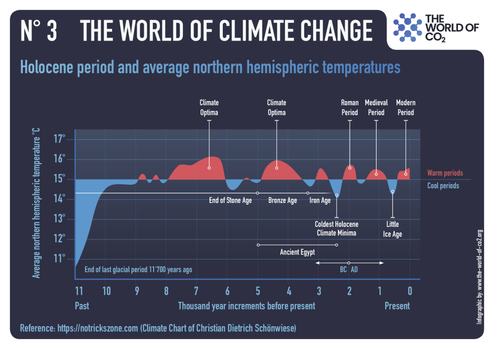
HS: When we talk about global warming, we say that the temperature might have got up by one degree or something like that. But if we look at geological time scales, the climate changes are much, much more severe. I mean, you have periods where you have glaciations, that is, ice almost down to the equator, and perhaps even most of the Earth is covered by ice, and you have periods where there’s no ice caps at all, and the temperature is much, much higher.  I mean, you have had… Beobab trees in Antarctica, and you had alligators at the latitude of Greenland.

So you have had much, much warmer, at least 10 degrees warmer climate back in time. So if we look at geological timescales, we have had enormous changes in climate. And of course, all of this is completely natural. And the question is, why did we have such big climate changes? And this is some of my work trying to understand why we have such large climate changes even back in time.

FR: So let’s talk about that. This is interesting that we’ve been told that the climate change today is anthropogenic. So let’s talk about your perspective on that and what does your research show?

HS: There’s no doubt that CO2 is a greenhouse gas and it has some effect on the temperature.The issue has to do with climate sensitivity. How big is the climate sensitivity? And it turns out that it’s probably around one degree if you double CO2.  So it’s a relatively benign effect of CO2. So, I’ve been working trying to understand why there are climate changes. When you look at climate changes, for instance, over the last 10,000 years, you can actually see that if you compare the climate changes with changes in solar activity, you actually find a very nice correlation.
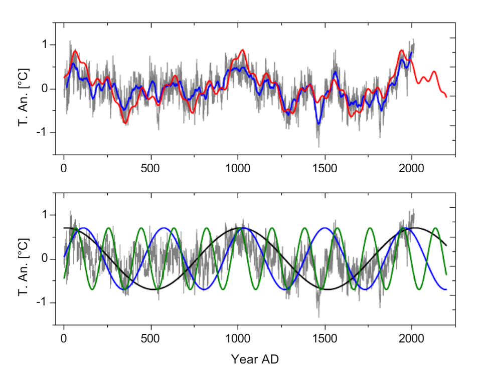
Fig. (3). (Color online) Upper panel: Global record G7 (grey), running 31 year average of G7 (blue), sine representation of G7 with three sine functions of the periods 1003, 463, and 188 years (green), with four sine functions including the period ~60 years (red), continued to AD 2200. The parameters of the sine functions are given in Table 3. The Pearson correlation between the 31 year running average of G7 and the three-sine representation (green) is 0.84, for the four-sine representation (red) 0.85. Lower panel: G7 (grey) together with the sine functions of 1003, 463, and 188 – year periods continued until AD 2200 (equal sine amplitudes for clarity) Source: Ludecke & Weiss 2019

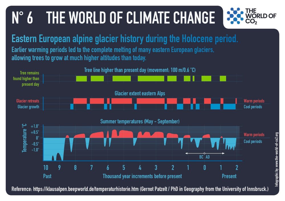
There are so many studies that show that you had, for instance, the Little Ice Age And you have the medieval warm period. And the medieval warm period is when you had a high solar activity. The little ice age is when the solar activity was low. And the question is, why should there be such a correlation?
How can the solar activity actually affect climate? And the simplest idea that has been put forward was that the output from the sun in the form of radiation, I mean the sunlight, that is changing. But it turns out that these changes are probably too small to explain what the climate changes you’re seeing.

So something else is going on, something is amplifying the solar activity and the idea that I came up with this now, actually 30 years ago, was that maybe solar activity is somehow regulating the Earth’s cloud cover. And initially, I took data from satellites that looked at the Earth’s cloud cover and I looked at it over a solar cycle that’s about 11 years and compared the changes in the solar cycle with changes in the Earth’s cloud cover. There seems to be a correlation between the two. So one can say that the idea, I mean, it looked as if it was something worth pursuing. But of course, it was just a correlation at that time.

Cosmic rays interacting with the Earth’s atmosphere producing ions that helps turn small aerosols into cloud condensation nuclei — seeds on which liquid water droplets form to make clouds. A proton with energy of 100 GeV interact at the top of the atmosphere and produces a cascade of secondary particles who ionize molecules when traveling through the air. One 100 GeV proton hits every m2 at the top of the atmosphere every second.

And I couldn’t say why there should be such a connection. So the general idea has to do with the formation of clouds. How are you actually forming clouds? And it turns out it’s the ionization that is happening in the atmosphere.  There’s typically about a thousand ions per cubic centimeter. So if you have a small cubic centimeter, you might have on the order of a thousand ions per cubic centimeter. And these ions are in general mainly produced because of very energetic particles that come from the Milky Way that is outside our solar system.

And they move in through the solar wind and then enter into the top of the atmosphere, where they then ionize the atmosphere. And the story is these small ions help stabilizing small molecular clusters. So you get what we call aerosols. These very small aerosols, which then grow up to a certain size. In order to make a cloud droplet, you have to have some kind of surface on which water vapor can condense. These small aerosols are actually providing these surfaces.

Cosmic Ray, Aerosol, Cloud Link
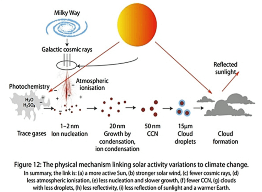
The idea is that if you have more cosmic rays coming into the atmosphere, you’re producing more of the small aerosols. They grow to become what we call cloud condensation nuclei, so they can affect the clouds, so water waves can condense and become cloud droplets. So if you have more cloud droplets, you have a more white cloud. And a more white cloud actually reflects the sunlight out to space again.
That is, of course, extremely important for the Earth’s energy balance. So that is the main idea behind the theory that I have been working on.
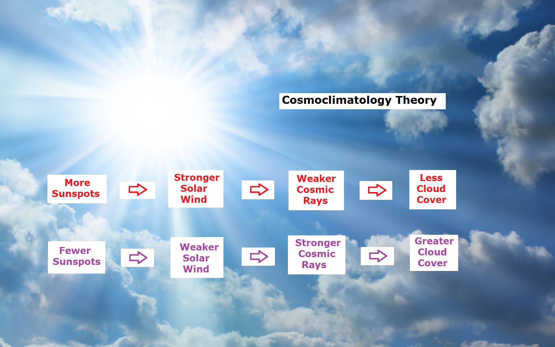
FR: Okay. And so if there is more clouds and reflect the sunlight back to space, I’m just gonna ask, I’m a lay person, not a scientist. Maybe I’m not, you know, a bit stupid question in that sense. But if it reflects more sunlight out, then well, logically, we get the cooler climate, right?

HS: Yes, exactly. Observations are one of the ways we can verify that it works. So on relatively rare occasions, there are some explosions at the sun. They’re called coronal mass ejections. It’s when the magnetic field lines sort of open up and the sun is throwing out a large magnetic plasma. And this magnetic plasma works more or less like an umbrella or a shield against the cosmic rays. So within a week, the cosmic rays are dropping, and they can drop maybe up to 30% or something like that. And that is like a natural experiment with the whole Earth.

And so you can actually then see if anything is happening with the Earth’s cloud cover. And this is something that we have investigated. So, for instance, we can also look at the aerosols that are produced after these events, and we can see that there is a big drop in the aerosols. And then we see a drop in the clouds following these events. And it’s not just the cloud fraction, it’s also the optical properties of clouds. So we can actually see changes in the cloud’s microphysics under these events.

So in some sense, we see the whole chain from the explosive events and the sun to changes in the cosmic rays to changes in the aerosols and then changes in the clouds. And there is a slight delay on a few days in the reaction. That’s simply because it takes about five days for the small aerosols to grow to become cloud condensation nuclei. So everything seems to be fitting very beautifully with respect to this idea.

FR: Okay. But, well, how frequently does it happen, what’s the correlation here? I mean, how frequently it happens to change the climate in that sense?

HS: I talked about this event with the explosions at the sun, which is something that happens during a week. So it’s too much too short to affect climate. But the solar activity modulates the cosmic rays. And that’s simply because the solar activity translates into changes in the solar wind. And the solar wind is covering the whole solar system and all the planets. That works like it’s a magnetic shield that screens against the cosmic rays.
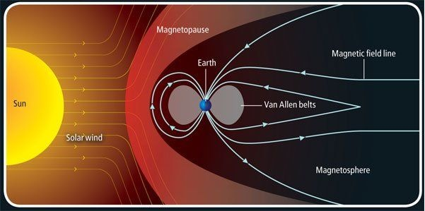
So when the solar activity is high, you can say that it’s screening better against the cosmic rays. That means you get fewer cosmic rays in to the atmosphere. So solar activity can regulate the amount of cosmic rays that comes into the atmosphere. So that regulates in the cloud cover. And we can then estimate, I mean, how much it changes the cloud cover during an 11-year cycle.

And from that, we can calculate what would be the effect on the temperature in the oceans. And there you actually see that we get about on the order of one to one and a half watt per square meter more energy in when you have a solar maximum than when you have a solar minimum.

And you can actually observe that in the ocean’s temperatures. You can see that in the heat content of the ocean. And you can even see it in the volume, because the heat goes in and out of the ocean. So when you get heat into the ocean, it expands a little bit.  So in the sea level, you can actually see an 11-year cycle in the sea level. And all of this, you can quantify how much energy goes in and out of the ocean.

And it fits very beautifully with what you expect from changes in the cloud cover over a solar cycle. And it’s interesting that the solar irradiance is almost a factor of 10 too small to explain it. So there is some kind of amplification mechanism. And the idea is that it’s clouds that are responsible for this. And this is something that you should takeway with respect to the ocean temperatures and the energy that goes in and out of the ocean he has been looking at.

FR: Okay. But how does it fit this idea? How does it fit the historical records?

Figure 4. The millennial solar-climate cycle over the past 2000 years. The anomaly in 14C production levels (black curve), a proxy for solar activity, is compared to iceberg activity in the North Atlantic (dashed blue curve), a climate proxy. The pink sine curve shows the millennial frequency. It defines two warm and two cold periods, supported by a large amount of evidence, some of which are represented by red and blue bars (see main text). Source: Javier Vinos

HS: Well,If you look at solar activity going back in time, we talked about the Little Ice Age, which is from around 1300 to 1850. And then you had the medieval warm period for 900 until maybe 1200. that these changes, they fit very beautifully with changes in cosmic rays. So when it’s cold, you have more cosmic rays coming in. And when it’s warm, you have less cosmic rays entering into the atmosphere. And we know these changes in cosmic rays because when cosmic rays enter the atmosphere, They are actually producing new elements like carbon-14, which is a radioactive form of carbon. It’s slightly heavier than carbon-12.

I guess many people know that you can use carbon-14 for dating things. But this carbon becomes CO2, the heavy form from carbon, and it goes into trees. And then you can look at the annual rings of the tree rings and measure how much carbon-14 you have relative to carbon-12.  And you can then measure that for all the tree rings going back in time and you can actually reproduce solar activity almost 20,000 years back in time. And if you look at these changes and you compare with how climate has been changing over that period, there is beautiful correlations again.

So it is near certain that there is a connection between solar activity and climate. And you can also quantify some of these changes and they are relatively big and it seems as if that, you know, changes in clouds is a very good candidate for explaining this. And when we look about the last 10,000 years, then the modulation of the cosmic rays, it’s caused by solar activity.

FR: Okay. Let me just ask you about those cosmic rays again. You did say, but again, I’m not that bright in your field. You did say it comes from Milky Way. Okay. Why does it come from there? Or what is it? What sends it here?

HS: Cosmic rays are very energetic particles. It’s mainly atomic nuclear, 90% is protons. So that’s the core of the hydrogen atom. So the energetic particles that we are interested in are mainly produced in what we call supernova. And a supernova, the case that we are interested in, is when you have a massive star that is maybe eight times or more massive than the sun. It only lives a relatively short period of time, you know, from maybe three million years to 40 million years.

So it’s a large star and it’s very heavy, and then in the process of burning, it burns so fast and it ends its life in a very, very violent explosion, which is called a supernova. And this supernova, when it explodes, it produces a shock front that is moving out from where the star was located. And this shock front, it works as, you can call it, a cosmic accelerator.

So it accelerates particles that move back and forth over this shock front and move them to extremely high energies. And the energies that you can obtain by this process is much higher than we can produce in any accelerator here on Earth artificially. And these particles, they are then moving in the interstellar space in the Milky Way.

And they are moving in the magnetic fields that are in between stars. So they are sort of moving like what we call diffusion. They are sort of randomly moving around, being bent by the magnetic fields. And then some of them will be outside, you know, arrive outside our solar system.

We have the heliosphere and then they move in and they feel the magnetic field from the sun. And some of them will then enter into the top of the atmosphere. And then you have maybe one proton that comes in with extremely high energy. And then it works a little bit like billiard ball where you have one particle hitting the molecules or the atoms in the atmosphere and it makes a shower, sort of a cascade of particles that goes down through the atmosphere. And these particles are called secondary particles. And so you can have one particle coming in that becomes millions and even billions of particles that move down through the atmosphere.

These particles are completely invisible to our naked eye.  While we are sitting here, we are penetrated by these secondary particles that go through my body and your body all the time. And so every 24 hours, maybe 20 million particles will go through your body and you don’t really experience this.  This is something that has happened since the formation of our galaxy. And of course, here on Earth, we have been showered with these particles for four and a half million years.

FR: Well, since you can explain past events with solar activity and how many cosmic rays are coming towards Earth, probably you can basically model what will happen as well, right? So, I mean, the question is, where are we now in terms of changing climate? Because I’ve also talked, for example, to Professor Zharkova. She said to me that we are entering another ice age soon.

HS: There’s no doubt that we will get an ice age. We have had a number of ice ages back in time. I don’t know if you’re talking about a real ice age or you’re talking about a little ice age, which is just a colder period.

FR: She was talking about the little ice age. I understood.

HS: So a little ice age. I know there are some predictions that the solar activity will go down and we might get a slightly colder period. I’m not sure it will be a little ice age, but it’s not something that I have looked at in any details. At the same time, of course we have had some heating from the CO2 increase in CO2. And then solar activity would then go the opposite way if the solar activity goes down. The problem with these predictions is that it’s extremely difficult to predict solar activity in the future.
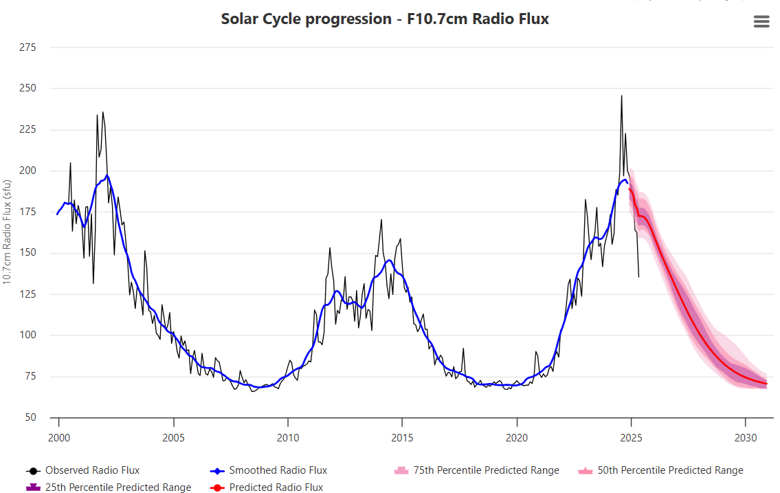
Source: spaceweatherlive

We can’t even predict the next solar cycle, whether it’s going to be high or low. There are some really amazing examples where this last solar cycle was predicted and the predictions were sort of all over the place. So it is really difficult to know because we don’t understand solar activity in a detail where we can predict what the next solar cycle will be. But that might come at some point. So something special has to happen. I think if we’re going to have a real cold period where the temperature drops by one or two degrees, that would be very special. I’m not sure that we’re going to see that, but I know that Zharkova is predicting that.

FR: Okay, yes. Anyhow, the thing is that still almost, well, all of it indicates that climate change is, there are some other factors than humans leading the climate change. But what is your opinion? What is the role of us on climate?

HS:  Oh, the anthropogenic CO2? Yeah. So as I said, it is a greenhouse gas. So you can see if you look at the outgoing long-wave spectrum, you can actually see there is a drop in the outgoing long-wave spectrum, which has to do with CO2, which means that it is a greenhouse gas.  The question is, how important is it? Is it so important that it’s changing temperature, you know, in a dramatic way? And I think there’s so much research now that seems to indicate that the climate sensitivity is on the order of, you know, one, maybe a little more than one degree for a doubling of CO2.

And that is much smaller than what you get from these climate models, which gives you between three and four degrees of that order, but at least a few times larger than what you get just from CO2 alone. Because in the climate models, the reason they get between three and four degrees is because they assume that it would be less cloudy, for instance, in the future climate. So you might have one degree from CO2, but then you get on the order of one or two degrees extra from what we call positive feedbacks. And that is something like more water vapour in the atmosphere or less clouds in a future climate.

And the problem is that water vapour and clouds are really the most uncertain thing about any prediction of climate. Clouds and aerosols are really what makes climate predictions so extremely difficult. And it’s because it’s all happening at length scales that are much, much smaller than what you can resolve in climate models.  You have to remember that you have maybe, you know, 50 to 100 kilometers between two grid points in a global numerical model.

And that means that, you know, if we just take Denmark, you have maybe one or two grid points over Denmark. And in each of these grid points, you have to determine, you know, what are the clouds actually just from temperature, humidity and pressure. So you have to do some kind of a parameterization of all the physics. So you’re not resolving clouds at all, but you are trying to use, you know, temperature and pressure to say what will the cloud look like for these variables. And this is basically impossible. I mean, it’s pure guesswork.

FR: So what do you think about those climate models? I mean, are they useful then at all?

HS: Of course, they’re useful for some things, but they’re not useful to say if the climate is going up by some fractions of degrees. And I don’t think you can use them for predicting future climate.

FR: But this is what they are used for, isn’t it?

HS: Yes, but I think also that there are some kind of a consensus that climate models are not doing well, I mean, that they have real problems in predicting and saying what is going to happen in the future. So they are not a crystal ball that can tell us about the future with very much accuracy.  Well, it depends on how you ask the questions, of course, but I think just recently there were some statements from people who are doing these models saying that they were running too warm.
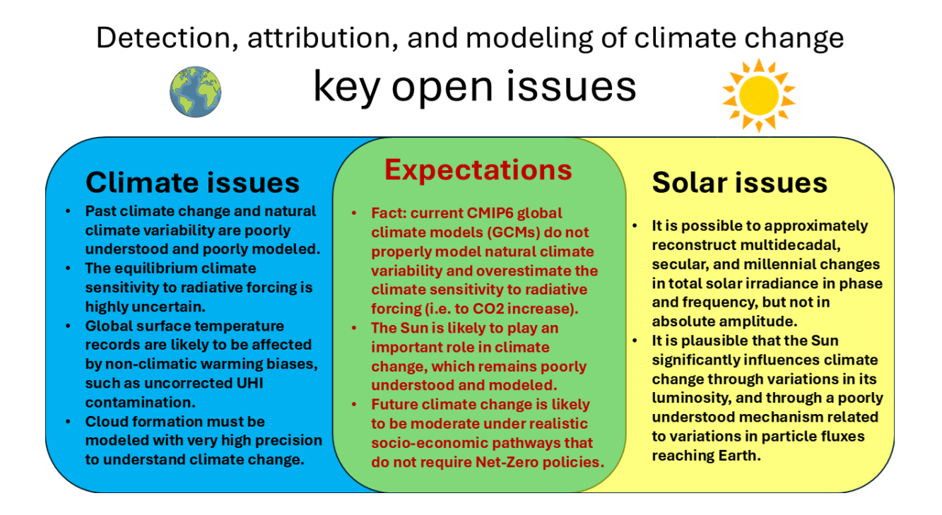
So they are, you know, exaggerating the warmth. And I think in one of them, there was because they updated their cloud scheme. So they changed the perameters of clouds. And all of a sudden, it was running slightly warmer than before. So again, it just points to the severe problem of clouds.  I should also say that if you take out clouds of the models, then the model results start agreeing with each other. Whereas when you have all the clouds in the models, then you get very different results from various models. I mean, it’s not like in particle physics where you have a standard model that you can use.

I mean, here you have a whole ensemble of the different models and they all give slightly different results. And then you make an ensemble average of all these models and try to say that that is the future. It’s, of course, not really satisfying.

FR: Of course. So what do you think about the reports that the UN IPCC puts forward, the scientific reports? Are they something that are, you know, accurate?

HS: I looked at it with respect to the things that I’m doing. One of the things that, you know, struck me was that if you look at the effect of the sun over the last hundred years, there is no effect whatsoever. I mean, it is so small that, I mean, they’re saying essentially that there’s no effect of changes in solar activity. really a shame in the sense that I mean, for instance, we see in the present climate that we’ve had over the last 50 years, you can see solar cycle variations in the ocean heat content and so on, which we talked about just before.

So the solar activity seems to be 10 times larger than what you get from solar irradiance. And in The reason that they get such a small effect of the sun is because they are only considering changes in solar irradiance, which has to do with the solar constant. The solar constant is changing, you know, about one tenth of one percent.  So that is so, so small that it does not have any effect on climate. However, the changes in… In clouds, if we take the ideas that I have been working with Nir Shaviv we will get that over the last century, over 120 years, I think at least one watt per square meter has entered because of solar activity.

Solar activity does not seem to have been completely negative as well. over the last 10 years.
So when we think about how the issue is approached, the issue of climate change in society now, well now there’s the new administration in the United States that actually approaches it somewhat different, but in the EU, for example, Mrs. von der Leyen said that she’s still determined to go to net zero and so on.

So what I mean here is the somewhat hysterical tone that this issue is approached with and also the predictions of doom. So my question is if it’s the same in the academia or not. I mean scientists are in my opinion, at least, they seem very rational and fact-based.  So, is it somewhat different in the inside, I mean, if you talk to your peers?

HS:  I usually say that climate science is not normal science. There’s so much politics involved, even in academia. There is a sort of self-censorship. It’s a bad career move to go against the idea that CO2 is the main driver or to say what i’m saying right now so it’s not good for your career to to do that it has implications, I mean first of all it’s the only research that is being financed that can be done, if you don’t get a grant or anything, you cannot do any research.

And that’s also why I think many people will not rock the boat, because it’s a good way of getting financing for the research that you want to do. However, if you try to do things which I have done, which is perceived as controversial and not according to the general ideas, it becomes very, very difficult to obtain funding and to survive in this system. And people are very emotional about this because some people think that they are trying to save the world from a disaster. And, you know they think everybody else has really bad motives, maybe hidden motives, your multinational oil companies or something like that.
So it’s really difficult to be in opposition to these ideas. So that it’s very, very difficult for me to obtain any funding. Some people are very upset, you know, if you have been invited for giving a talk and some people find out who you are. and so on. So there’s many, many strange things happening.

FR: It’s really happening, right? I mean, it has happened to you that you’re invited to give a talk to talk about your research and there are activists who are coming to cancel you. Did I understand correctly?

Antifa thugs outside Munich Conference Center at 2019 Climate Meeting.

HS: Yes. I’ve also given talks in Germany, where the whole conference had to have police protection because of the demonstrators that tried to storm the place. Another time, on the building, they printed that we were Nazis and they put glue in the locks and so on.  Yes, so one couldn’t get in. I mean, it’s just sometimes it’s very, very, very strange how emotional it is. And there’s nothing rational about it because it’s not something that you can have a discussion about. I mean, you also heard people saying that, you know, the science has been done. Now it’s only action that is needed.

FR: Yes, yes. Well, it’s being parroted all the time. I don’t know, is it 100% already or last time I checked it was 99% of climate scientists agree on something.

HS: But all of these things are simply propaganda of some kind. It has no sort of basis in reality. It’s just some talking points that are being spread out. And some people believe them and other people know that they’re not entirely correct. And that’s how it is.

But the good thing is that I tried to survive in this system. Then I started to look at very, very long timescales. And I think, I mean, maybe we should I should tell you just a few words about that, because I think it’s a completely fascinating result that has come out. Absolutely.

So we talked about these supernovas that goes off, and they are producing the cosmic rays. So you can say supernovas are the source of cosmic rays. And the interesting thing is that our solar system it is actually moving around the Milky Way galaxy. So we are in a spiral galaxy, so it’s like a flat thing.
And we are moving around the center of the galaxy, the whole solar system, within 240 million years or 230 million years it takes. Our Milky Way is a spiral galaxy. And in these spiral arms, that’s actually where you have a lot of star formation. And star formation is where you also produce the large, heavy stars that explode.
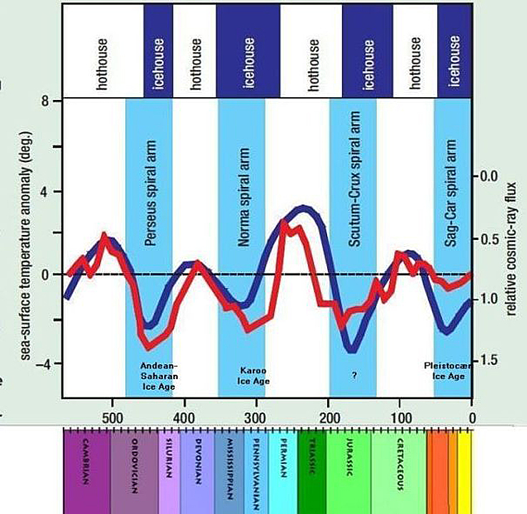
Cosmic radiation and temperature through Phanerozoic according to Nir Shaviv and Jan Veizer. Blue columns refer to Milky Way Spiral arms.

So that means that when the solar system goes through a spiral arm, it actually in an area with much higher cosmic rays, Whereas when you are in between spiral arms, you have much lower. And the changes are not 10, 20% like we have from solar activity.

Now we are talking about several hundred percent of changes in the cosmic rays. So you can say that this is a completely independent way of testing the cosmic ray climate mechanism. Because if these changes in cosmic rays are important for climate, as we see in the present time, maybe they should also be important when we go back in time. It’s something that Nir Shviv actually looked at around 2001.

And what you find is that when you are in a spiral arm, it tends to be extremely cold on Earth. So the glaciations that we have had on Earth on cold periods fit beautifully when we were in spiral arms. And when we were in between the spiral arms, it was extremely warm. The temperature changes and the climate changes we are talking about are now, you know, from what we call an ice house, that is the glaciation, very severe glaciations, that is the large ice sheets on the Earth, to where they are completely melted and, you know, the sea level has gone up maybe by 100 meters or something like that. So it’s enormous changes.

What I looked for was to see if it has implications for life on Earth. And it turns out that you can actually indirectly look at how big the biomass has been at certain times in the ocean. And that is because you can look at organic material. So when you have the ocean and you have organic material, some of the dead material falls down at the bottom. And you can actually say something about the fraction of organic carbon relative to inorganic carbon in sediments.

So when you have sedimented mountains, you can go and measure this ratio of organic carbon to inorganic carbon. And it says something about the fraction of organic material that has been buried in sediments. And it turns out when you look at this fraction as a function of time, It fits beautifully with changes in reconstructed changes in supernovae.
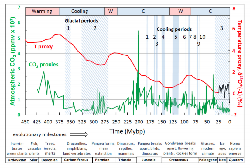
And you can actually see it in fairly high details over the last 500 million years. And it turns out that you can actually extend it. So from geology, you have this fraction of organic material almost four and a half billion years back in time. And even here, it fits beautifully with the changes in the cosmic rays that have happened over the whole history of the Earth. It’s completely astounding that you have this correlation over four and a half billion years. So it says that the biomass seems to have been following things which are thousands of light years away from our solar system.

So this star formation has actually influenced the conditions for life. And it’s even more interesting because when you bury organic material, the organic material is made because of photosynthesis. And photosynthesis, that is, you know, the algaes, the green algaes produce oxygen.  So you have CO2 and water and sunlight that becomes, you know, sugar and oxygen. But in order for the reaction not to go back again, so the oxygen becomes CO2, you actually have to take the organic material and then have the oxygen and you bury the organic material in the sediments.

That’s the way you get the oxygen. So these variations in the organic material, these variations, they are actually also the production of oxygen that we have had over the whole history of the Earth. So supernovas have therefore indirectly produced or been responsible for changing the oxygen at Earth and all complex life.  I mean, in order to get complex life, we need oxygen. So it’s really been a very important part. So it seems to say that the Earth is really a part of an ecosystem, you know, where it really involves most of the galaxy. So here we see that it fits beautifully with the changes in cosmic rays or supernova frequency over most of the history of the Earth.
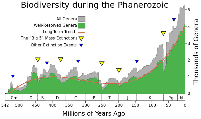
Source: Phanerozoic_Biodiversity.png Author: SVG version by Albert Mestre

I did another thing where I looked at the diversity of life, and just to cut the thing relatively short, it turns out that there’s a beautiful signal of the supernova frequency, even in the frequency, in the diversity of life, where you can see a very, very beautiful correlation over the last 500 million years. So it suggests that somehow the changes in the supernova  change the climate. And by changing the climate, if it’s colder, you have a larger temperature difference between equator and polar regions.

That means you have stronger winds. And if the wind is stronger, then you have more mixing in the oceans. And what it is mixing is the nutrients that life actually needs. I mean, a lot of the nutrients, they run out from rivers because of rain. And you have, you know, phosphorus and iron and oxygen. and other important elements for life. But they are then transported so life can uptake these nutrients. And the idea is that when you have more nutrients, then you can also have a higher diversity and you also get the higher biomass and you get more sediments. So everything seems to be connected in that way. I hope this was not too complicated.

FR: Well, I mean, yes, I think it wasn’t too complicated, but it’s really interesting to actually hear about the research, yes, and to think about the connections that you pointed out there. So, the only thing I would like to ask here is that, so it’s a hypothesis, of course, and again, how… how it is welcomed in your circles? I mean, is there any discussion about it or how it is approached?

HS: I think in geology and geologists, there’s a lot of geologists that really like it because many of them, they have seen how climate is changing over these long timescales and, you know, some of them, they know that CO2 does not appear to be the driver of climate changes on these long timescales. But I should also say that even in geology, there are people who are promoting that everything should be CO2, that CO2 is also driving climate on these very long timescales. But there are many places where it simply does not fit. So I don’t think that… I don’t think it’s a good theory.

I mean, you typically hear about, for instance, having extremely high CO2 levels at the same time that you had an ice age. And there are some problems also within the last 30 million years where CO2 actually dropped a lot. There are periods where temperature actually goes up and so you don’t have this correlation over many million years and some of it is called a climate paradox. There are some problems.

FR: Yes, of course, of course. Yes. So, I mean, it has been really nice talking to you, but I can see that our time for today is almost running out. I mean, thank you really for this interesting conversations and for the insights and for talking about your research in detail.  I hope my audience also listens and can hear some, well, good ideas, but they’re not only ideas because, well, this is what science actually must look like, ask questions and try to find answers, correct?

HS: Yes, I agree, that’s what we try to do.


Arctic Ice Aplenty at Annual Dip September 2025

After a sub-par March maximum, by end of May 2025 Arctic ice closed the gap with the 19-year average.  In mid-August MASIE showed the Arctic ice extent matching the 19-year average.  Mid month Arctic ice went above average and remained in surplus, ranging from a high of +231k km2 to +160k km2 at end of August. Now during the annual minimum month of September 2025 there is  Arctic ice aplenty.

During the annual dip in Arctic ice extent, the average year since 2006 is lowest on day 260 at 4.53M km2.  It then rises to 4.8M km2 ten days later.  The cyan line shows 2025 above average throughout, its lowest extent at 4.85M km2 on day 265, and now up to 5.07M km2.  SII v.4 was lower than MASIE throughout, but has drawn closer in recent days.  So far MASIE September average is 5.0M and SII is 4.7M, with 4 more days remaining in the month. Note 2007 was ~800k km2 in deficit, 2020 ~600k down at day 270, while last year was ~300k below average.

The regional distribution of ice extents is shown in the table below. (Bering and Okhotsk seas are excluded since both are now virtually open water.)

Region 2025270 Day 270 ave. 2025-Ave. 2007270 2025-2007
 (0) Northern_Hemisphere 5074777 4798758 276018 4023569 1051207
 (1) Beaufort_Sea 483527 520730 -37203 482030 1497
 (2) Chukchi_Sea 332213 210352 121861 214 331999
 (3) East_Siberian_Sea 499915 280923 218992 311 499604
 (4) Laptev_Sea 273431 152794 120636 238340 35091
 (5) Kara_Sea 4906 33680 -28774 15113 -10207
 (6) Barents_Sea 0 12945 -12945 4851 -4851
 (7) Greenland_Sea 165160 225916 -60756 339720 -174560
 (8) Baffin_Bay_Gulf_of_St._Lawrence 70284 47480 22804 43624 26660
 (9) Canadian_Archipelago 302771 336303 -33533 280360 22410
 (10) Hudson_Bay 2415 2252 163 1936 479
 (11) Central_Arctic 2938588 2974115 -35527 2615795.38 322792

The table shows large surpluses in Eurasian basins  Laptev, Chukchi and E. Siberian, more than offsetting smaller deficits in Central Arctic, CAA and Greenland seas. Hudson Bay is mostly open water at this time of year. 2025 exceeds the average ice extents by 276k km2, or 6%, and is over 1 wadham greater than 2007 or a surplus of 1.05M km2 of ice extent.

September monthly average ice extent is considered the annual minimum for climate purposes.  Note also that typically the lowest daily value occurs mid September, with a small positive gain between the end of August and end of September.

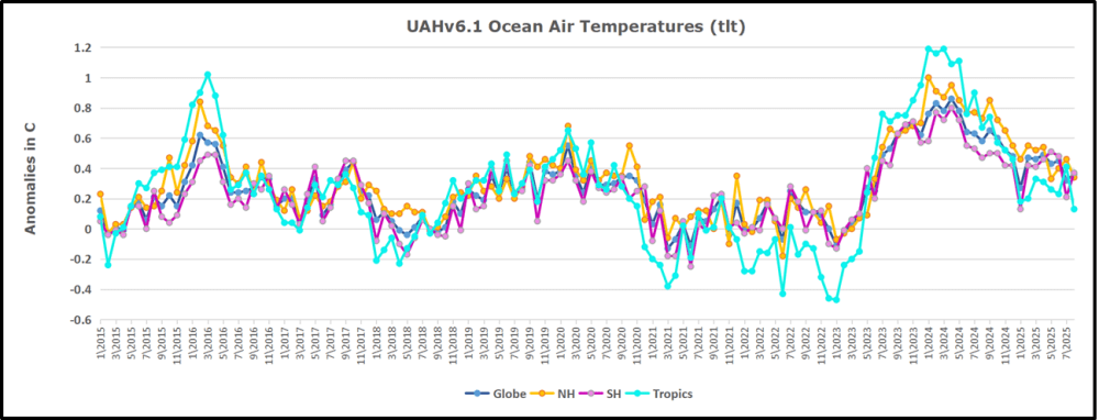
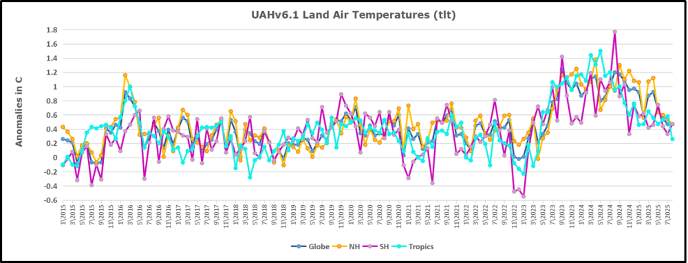
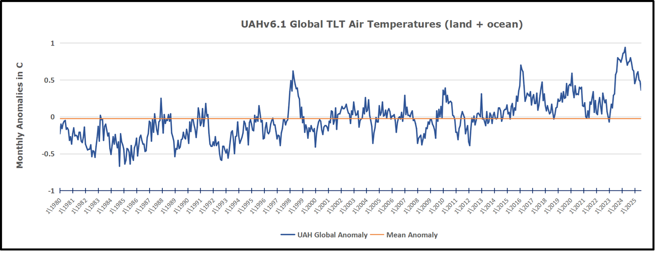
Why is this important?  All the claims of global climate emergency depend on dangerously higher  temperatures, lower sea ice, and rising sea levels.  The lack of additional warming prior to 2023 El Nino is documented in a post SH Drives UAH Temps Cooler July 2025.

The lack of acceleration in sea levels along coastlines has been discussed also.  See Observed vs. Imagined Sea Levels 2023 Update

Also, a longer term perspective is informative:

post-glacial_sea_level

Footnote Regarding  SII v.4

NSDIC acknowledged my query regarding the SII (Sea Ice Index) dataset. While awaiting an explanation I investigated further. My last download of the SII Daily Arctic Ice Extents was on July 30, meaning that the most recent data in that file was day 210, July 29. The header on that file was Sea_Ice_Index_Daily_Extent_G02135_v3.

Then on August 1, the downloaded file had the heading Sea_Ice_Index_Daily_Extent_G02135_v4. So it appears that these are now the values from a new version of SII. As I wrote in my query, since March 14 all of the values for Arctic Ice Extents are lower in this new record. The graph above shows the implications for August as an example of estimates from SIIv.4.

In the past, SIIv.3 tracked MASIE with slightly lower values.  But with v.4, larger monthly average deficits to MASIE were reported in July 2025 ( -282k km2) and in August (-440k km2).

The change started in January 2025 and will be the basis for future reporting.  The logic for this is presented in this document: Sea Ice Index Version 4 Analysis

In June 2025, NSIDC was informed that access to data from the Special Sensor Microwave
Imager/Sounder (SSMIS) onboard the Defense Meteorological Satellite Program (DMSP)
satellites would end on July 31 (NSIDC, 2025). To prepare for this, we rapidly developed version
4 of the Sea Ice Index. This new version transitions from using sea ice concentration fields
derived from SSMIS data as input to using fields derived from the Advanced Microwave
Scanning Radiometer 2 (AMSR2) sensor onboard the Global Change Observation Mission – W1
(GCOM-W1) satellite.  On 29 July 2025, we learned that the Defense Department decision to terminate access to DMSP data had been reversed and that data will continue to be available until September 2026.

We are publishing Version 4, however, for these reasons:

• The SSMIS instruments are well past their designed lifespan and a transition to
AMSR2 is inevitable. Unless the sensors fail earlier, the DoD will formally end the
program in September 2026.
• Although access of SSMIS will continue through September 2026, the Fleet
Numerical Meteorology and Oceanography Center (FNMOC), where SSMIS data
from the DMSP satellite are downloaded, made an announcement that “Support
will be on a best effort basis and should be considered data of opportunity.” This
means that SSMIS data will likely contain data gaps.
• We have developer time to make this transition now and may not in the future.
• We are confident that Version 4 data are commensurate in accuracy to those
provided by Version 3.

Advance Briefing for COP30 Belém 2025


Overview from E Co. A summit at the crossroads

When the world gathers in Belém, Brazil, in November 2025 for COP30, it won’t be just another climate conference. It will be the first major summit after the Paris Agreement’s initial Global Stocktake at COP28, and the moment where climate ambition must decisively shift from words to delivery.

As many observers have begun to remark in the run-up to COP30, “Belém is where the climate community will be asked to prove that promises can become practice.”

What’s at stake at COP30

The Brazilian presidency has laid out a clear mandate: COP30 must focus on implementation, inclusion, and innovation. In practical terms, that means:

♦  A ‘Belém Package’ of outcomes across forests, finance, adaptation, just transition, and gender.
♦  The formal launch of the Tropical Forest Forever Facility (TFFF), a proposed $125 billion results-based finance mechanism to incentivise forest conservation.
♦  Progress on a roadmap to mobilize $1.3 trillion annually in climate finance by 2035, building on the ‘Baku to Belém’ finance commitments made at COP29.
♦  New modalities for inclusive governance, such as Brazil’s proposed ‘Global Mutirão’, bringing Indigenous peoples, local governments, and civil society closer to the heart of climate decision-making .

COP30 will not be judged by the number of new pledges it produces. As several analysts have argued, it will be remembered “for whether the world found the tools to finally deliver on them.”

The main challenges Brazil faces

While Brazil has bold ambitions for COP30, turning them into concrete outcomes will not be easy. The presidency faces several challenges:

  1. Domestic contradictions: Despite progress under President Lula, agribusiness and mining interests remain powerful drivers of deforestation. Balancing economic pressures with climate leadership will test political resolve.
  2. Financing the transition: Brazil is pushing for massive climate finance scaling, but securing commitments for the $1.3 trillion annual target will be politically contentious, especially given donor fatigue and fiscal constraints in developed economies.
  3. Geopolitical polarisation: COP30 is the first climate summit taking place without strong U.S. engagement, given Washington’s announced withdrawal from the Paris Agreement in 2026 . This leaves Brazil trying to mediate between the EU, China, BRICS, and vulnerable countries, all with diverging agendas.
  4. Institutional fragility: While Brazil champions new governance ideas like a UN Climate Change Council, consensus on reforming multilateral processes is difficult. Many countries remain wary of ceding more authority to new structures.
  5. Logistics and credibility: Hosting COP30 in Belém is symbolically powerful but practically challenging. The Amazonian city faces infrastructure constraints, raising concerns about logistics, inclusivity, and whether Brazil can deliver an event of this scale smoothly.

“Brazil has set the bar high. But if expectations outpace deliverables, COP30 risks being remembered as another missed opportunity.”

My Comments

Since there is a big push on climate funding, maybe they could get to the bottom of this.

Maybe donors are put off by no one knowing who gets the money and for what it is spent.  And while they are investigating, how about understanding Energy Return on Investment (EROI): you know, the notion that an energy project is worth doing if the energy produced is greater than energy spent.  The poster at the top reminds of people dreaming of a world free of fossil fuels.

Why a COP Briefing?

Actually, climate hysteria is like a seasonal sickness.  Each year a contagion of anxiety and fear is created by disinformation going viral in both legacy and social media in the run up to the annual autumnal COP.  Since the climatists are especially desperate with the US outspokenly against the climate movement, we can expect the public will be hugely hosed with alarms over the next few weeks.  Before the distress signals go full tilt, individuals need to inoculate themselves against the false claims, in order to build some herd immunity against the nonsense the media will promulgate. This post is offered as a means to that end.

Media Climate Hype is a Cover Up

Back in 2015 in the run up to Paris COP, French mathematicians published a thorough critique of the raison d’etre of the whole crusade. They said:

Fighting Global Warming is Absurd, Costly and Pointless.

  • Absurd because of no reliable evidence that anything unusual is happening in our climate.
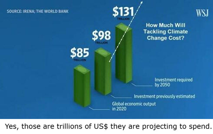
  • Costly because trillions of dollars are wasted on immature, inefficient technologies that serve only to make cheap, reliable energy expensive and intermittent.
  • Pointless because we do not control the weather anyway.

The prestigious Société de Calcul Mathématique (Society for Mathematical Calculation) issued a detailed 195-page White Paper presenting a blistering point-by-point critique of the key dogmas of global warming. The synopsis with links to the entire document is at COP Briefing for Realists

Even without attending to their documentation, you can tell they are right because all the media climate hype is concentrated against those three points.

Finding: Nothing unusual is happening with our weather and climate.
Hype: Every metric or weather event is “unprecedented,” or “worse than we thought.”

Finding: Proposed solutions will cost many trillions of dollars for little effect or benefit.
Hype: Zero carbon will lead the world to do the right thing.  Anyway, the planet must be saved at any cost.

Finding: Nature operates without caring what humans do or think.
Hype: Any destructive natural event is blamed on humans burning fossil fuels.

How the Media Throws Up Flak to Defend False Suppositions

The Absurd Media:  Climate is Dangerous Today, Yesterday It was Ideal.

Billions of dollars have been spent researching any and all negative effects from a warming world: Everything from Acne to Zika virus.  A recent Climate Report repeats the usual litany of calamities to be feared and avoided by submitting to IPCC demands. The evidence does not support these claims. An example:

 It is scientifically established that human activities produce GHG emissions, which accumulate in the atmosphere and the oceans, resulting in warming of Earth’s surface and the oceans, acidification of the oceans, increased variability of climate, with a higher incidence of extreme weather events, and other changes in the climate.

Moreover, leading experts believe that there is already more than enough excess heat in the climate system to do severe damage and that 2C of warming would have very significant adverse effects, including resulting in multi-meter sea level rise.

Experts have observed an increased incidence of climate-related extreme weather events, including increased frequency and intensity of extreme heat and heavy precipitation events and more severe droughts and associated heatwaves. Experts have also observed an increased incidence of large forest fires; and reduced snowpack affecting water resources in the western U.S. The most recent National Climate Assessment projects these climate impacts will continue to worsen in the future as global temperatures increase.

Alarming Weather and Wildfires

But: Weather is not more extreme.


And Wildfires were worse in the past.
But: Sea Level Rise is not accelerating.

post-glacial_sea_level

Litany of Changes

Seven of the ten hottest years on record have occurred within the last decade; wildfires are at an all-time high, while Arctic Sea ice is rapidly diminishing.

We are seeing one-in-a-thousand-year floods with astonishing frequency.

When it rains really hard, it’s harder than ever.

We’re seeing glaciers melting, sea level rising.

The length and the intensity of heatwaves has gone up dramatically.

Plants and trees are flowering earlier in the year. Birds are moving polewards.

We’re seeing more intense storms.

But: Arctic Ice has not declined since 2007.

But: All of these are within the range of past variability.In fact our climate is remarkably stable, compared to the range of daily temperatures during a year where I live.

And many aspects follow quasi-60 year cycles.

The Impractical Media:  Money is No Object in Saving the Planet.

Here it is blithely assumed that the UN can rule the seas to stop rising, heat waves to cease, and Arctic ice to grow (though why we would want that is debatable).  All this will be achieved by leaving fossil fuels in the ground and powering civilization with windmills and solar panels.  While admitting that our way of life depends on fossil fuels, they ignore the inadequacy of renewable energy sources at their present immaturity.

An Example:
The choice between incurring manageable costs now and the incalculable, perhaps even irreparable, burden Youth Plaintiffs and Affected Children will face if Defendants fail to rapidly transition to a non-fossil fuel economy is clear. While the full costs of the climate damages that would result from maintaining a fossil fuel-based economy may be incalculable, there is already ample evidence concerning the lower bound of such costs, and with these minimum estimates, it is already clear that the cost of transitioning to a low/no carbon economy are far less than the benefits of such a transition. No rational calculus could come to an alternative conclusion. Defendants must act with all deliberate speed and immediately cease the subsidization of fossil fuels and any new fossil fuel projects, and implement policies to rapidly transition the U.S. economy away from fossil fuels.

But CO2 relation to Temperature is Inconsistent.

But: The planet is greener because of rising CO2.

But: Modern nations (G20) depend on fossil fuels for nearly 90% of their energy.

But: Renewables are not ready for prime time.

People need to know that adding renewables to an electrical grid presents both technical and economic challenges.  Experience shows that adding intermittent power more than 10% of the baseload makes precarious the reliability of the supply.  South Australia is demonstrating this with a series of blackouts when the grid cannot be balanced.  Germany got to a higher % by dumping its excess renewable generation onto neighboring countries until the EU finally woke up and stopped them. Texas got up to 29% by dumping onto neighboring states, and some like Georgia are having problems.

But more dangerous is the way renewables destroy the economics of electrical power.  Seasoned energy analyst Gail Tverberg writes:

In fact, I have come to the rather astounding conclusion that even if wind turbines and solar PV could be built at zero cost, it would not make sense to continue to add them to the electric grid in the absence of very much better and cheaper electricity storage than we have today. There are too many costs outside building the devices themselves. It is these secondary costs that are problematic. Also, the presence of intermittent electricity disrupts competitive prices, leading to electricity prices that are far too low for other electricity providers, including those providing electricity using nuclear or natural gas. The tiny contribution of wind and solar to grid electricity cannot make up for the loss of more traditional electricity sources due to low prices.

These issues are discussed in more detail in the post Climateers Tilting at Windmills

The Irrational Media:  Whatever Happens in Nature is Our Fault.

An Example:

Other potential examples include agricultural losses. Whether or not insurance
reimburses farmers for their crops, there can be food shortages that lead to higher food
prices (that will be borne by consumers, that is, Youth Plaintiffs and Affected Children).
There is a further risk that as our climate and land use pattern changes, disease vectors
may also move (e.g., diseases formerly only in tropical climates move northward).36 This
could lead to material increases in public health costs

But: Actual climate zones are local and regional in scope, and they show little boundary change.

But: Ice cores show that it was warmer in the past, not due to humans.

The hype is produced by computer programs designed to frighten and distract children and the uninformed.  For example, there was mention above of “multi-meter” sea level rise.  It is all done with computer models.  For example, below is San Francisco.  More at USCS Warnings of Coastal Floodings

In addition, there is no mention that GCMs projections are running about twice as hot as observations.

Omitted is the fact GCMs correctly replicate tropospheric temperature observations only when CO2 warming is turned off.

Figure 5. Simplification of IPCC AR5 shown above in Fig. 4. The colored lines represent the range of results for the models and observations. The trends here represent trends at different levels of the tropical atmosphere from the surface up to 50,000 ft. The gray lines are the bounds for the range of observations, the blue for the range of IPCC model results without extra GHGs and the red for IPCC model results with extra GHGs.The key point displayed is the lack of overlap between the GHG model results (red) and the observations (gray). The nonGHG model runs (blue) overlap the observations almost completely.

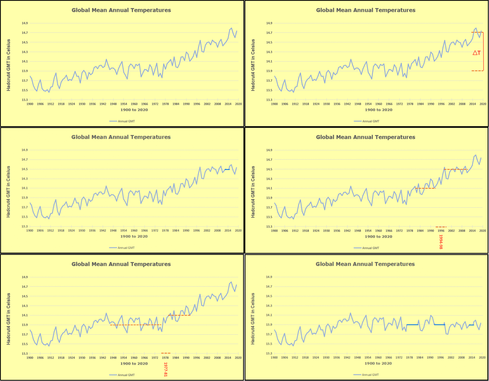
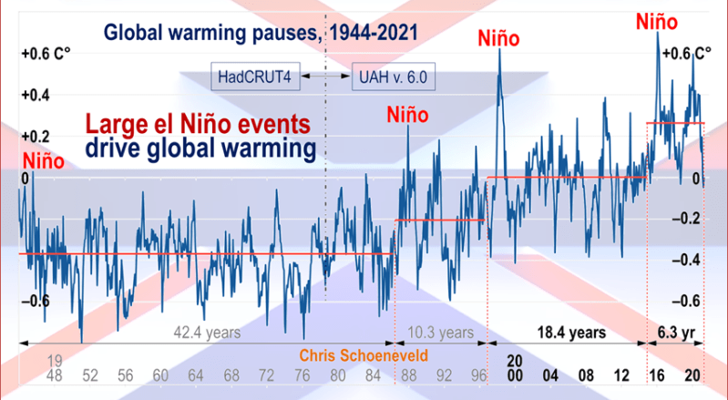
In the effort to proclaim scientific certainty, neither the media nor IPCC discuss the lack of warming since the 1998 El Nino, despite two additional El Ninos in 2010 and 2016, plus an unexplained spike in 2023-24, now cooling off.

Further they exclude comparisons between fossil fuel consumption and temperature changes. The legal methodology for discerning causation regarding work environments or medicine side effects insists that the correlation be strong and consistent over time, and there be no confounding additional factors. As long as there is another equally or more likely explanation for a set of facts, the claimed causation is unproven. Such is the null hypothesis in legal terms: Things happen for many reasons unless you can prove one reason is dominant.

Finally, advocates and IPCC are picking on the wrong molecule. The climate is controlled not by CO2 but by H20. Oceans make climate through the massive movement of energy involved in water’s phase changes from solid to liquid to gas and back again. From those heat transfers come all that we call weather and climate: Clouds, Snow, Rain, Winds, and Storms.

Esteemed climate scientist Richard Lindzen ended a very fine recent presentation with this description of the climate system:

I haven’t spent much time on the details of the science, but there is one thing that should spark skepticism in any intelligent reader. The system we are looking at consists in two turbulent fluids interacting with each other. They are on a rotating planet that is differentially heated by the sun. A vital constituent of the atmospheric component is water in the liquid, solid and vapor phases, and the changes in phase have vast energetic ramifications. The energy budget of this system involves the absorption and reemission of about 200 watts per square meterDoubling CO2 involves a 2% perturbation to this budget. So do minor changes in clouds and other features, and such changes are common. In this complex multifactor system, what is the likelihood of the climate (which, itself, consists in many variables and not just globally averaged temperature anomaly) is controlled by this 2% perturbation in a single variable? Believing this is pretty close to believing in magic. Instead, you are told that it is believing in ‘science.’ Such a claim should be a tip-off that something is amiss. After all, science is a mode of inquiry rather than a belief structure.

Summary:  From this we learn three things:

Climate warms and cools without any help from humans.
Warming is good and cooling is bad.
The hypothetical warming from CO2 would be a good thing.


Climate Medical Quackery Exposed

The following 65 page report was Submitted September 19, 2025 by physicians Dr. D. Weston Allen, Dr. Jan Breslow, and Dr. Daniel Nebert CO2 Coalition Comment on Reconsideration of 2009 Endangerment Finding and Greenhouse Gas Vehicle Standards  Excerpts in italics with my bolds and added images.

Table of Contents
Climate Change and Health …………………………………………………………………………………… 3
Introduction……………………………………………………………………………………………………. 3
Warmth, Wealth and Health……………………………………………………………………………….. 3
Temperature, Morbidity and Mortality ………………………………………………………………….. 6
Future Warming ……………………………………………………………………………………………. 10
Temperature Extremes…………………………………………………………………………………….. 12
Temperature and Disease Vectors………………………………………………………………………. 15
Extreme Weather Events………………………………………………………………………………….. 24
Food, Famine, Climate and CO2 ………………………………………………………………………….. 33
Mental Health……………………………………………………………………………………………….. 37
Energy Sources and Health……………………………………………………………………………….. 39
Conclusion……………………………………………………………………………………………………. 44
References……………………………………………………………………………………………………. 45

Some examples of Climate Medical Mischief

Introduction

Human health, morbidity, mortality and longevity are significantly impacted by climate. This review examines the evidence for past, present and possible future human health impacts of climate change and its ramifications. It will also examine the health impacts of different energy sources and climate actions. It will not examine every link in the literature to a range of conditions where attribution is implausible or tenuous, or where association assumes causation.

Warmth, Wealth and Health

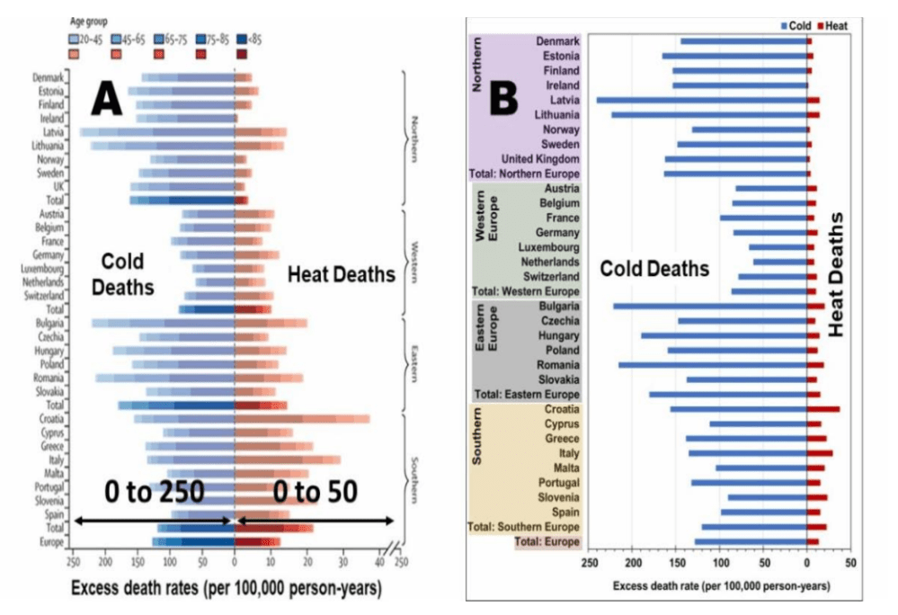
Davis et al (2003)23 found a 74.4% decline in heat-related mortality in 28 of the largest U.S. cities from 1964 to 1998 and estimated that another 1⁰C increase would further reduce the net mortality rate.24 Analyzing over 74 million deaths in 384 locations across 13 countries, Gasparrini et al (2015)25 found that cold weather was over 17 times more lethal than hot weather: 7.3% of all deaths due to cold and 0.42% from heat. Masselot et al (2023) found cold weather to be ten times more lethal than hot weather across Europe and forty times more so in northern Europe.26 Their visual display of this difference (Fig. 1) was camouflaged by making the X-axis for heat-related deaths 5.6 times greater than the X-axis for cold-related deaths!

Figure 1: Temperature-related mortality in European cities from Masselot et al. 2023 (A) As depicted in the Lancet (B) Identical X-axis for heat and cold, corrected by the CO2 Coalition

Temperature and Diseases

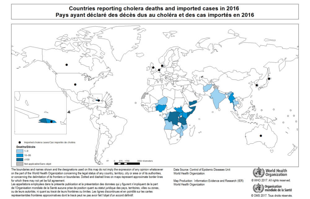
Cholera, which afflicts 3-5 million people and kills about 100,000 annually,76 is now confined to developing countries in the tropics and subtropics (Fig. 5). When an epidemic broke out in London in 1848, Dr. John Snow performed the world’s first epidemiological studies in linking itto contaminated water. Nearly a century and a half later, a paper in the prestigious journal Science77 linked a 1991 outbreak in South America to climate change. The real cause, however, was a failure of the Peruvian authorities to properly chlorinate water supplies.78 Climate change can be a convenient scapegoat for government failure!

Temperature Extremes

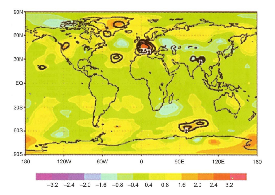
Deadly heatwaves such as the European one in 2003 are often attributed to climate change.93
Temperatures elsewhere across the globe at the time, however, were normal or below normal (Fig.
7).94

Figure 7: Global tropospheric temperature anomalies, June-August 2003. Source: Chase et al. (2006)

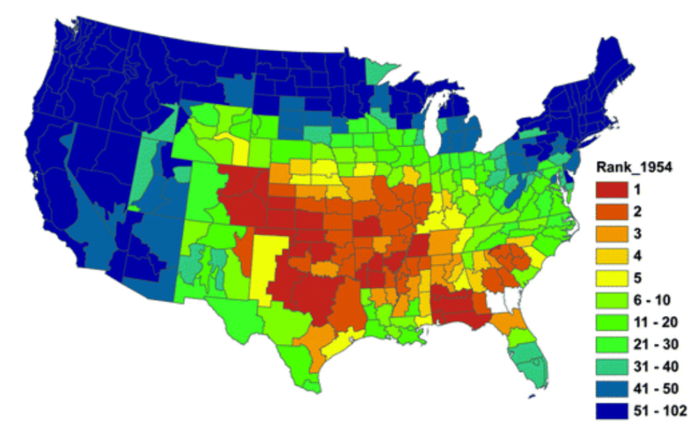
The 1936 North American heatwave during the Dust Bowl decade set record temperatures across 14 states, reaching 49⁰C in Steele, North Dakota, and killed at least 5,000 people.99 The 1954 summer-long heatwave across the Midwest, reaching 117⁰F (47.2⁰C) in East St Louis, ranks as the hottest in 11 states (Fig. 8) based on an analysis of Midwest temperature records from 1845 to 2009.100 Nancy Westcott (2011) also found a reducing trend of heatwaves over the 20th century.

Figure 8: Rank of the June–September 1954 heat wave based on National Climatic Data Center (NCDC) climate division temperature data for the years 1895–2009. Source: Westcott (2011)

Temperature and Disease Vectors

West Nile Virus (WNV) was first identified in a West Nile district of Uganda in 1937. It is asymptomatic in 80% of infected people but can cause severe encephalitis or meningitis in about 1 in 150 infected persons, especially the elderly or immunocompromised. It is transmitted by a Culex species of mosquito that has bitten an infected bird (not human). Appearing in New York in 1999 and spreading across the states taking hundreds of lives, it was soon linked to climate change. 173 174 But its rapid spread from northeast to the south and west (Fig. 12) and its decline despite warming (Figs. 13 and 14) indicates that the vector was already there and climate change had nothing to do with that.

Figure 12: Progress of WNV in the U.S. 1999-2003. White 0, Blue <1%, Green1-5%, Yellow 5-10%, Red >10%

Food, Famine, Climate and CO2

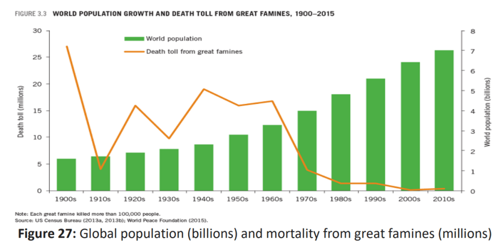
In his 1968 book The Population Bomb, Paul Ehrlich predicted widespread famine with hundreds of millions starving to death in the 1970s, but the death toll declined as the population grew
(Fig. 27).

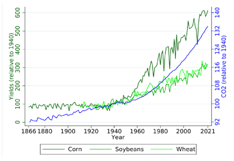
The U.S. National Bureau of Economic Research matched satellite-based observations of outdoor CO2 levels across the U.S. with county-level agricultural output data and other economic variables and concluded that CO2 emissions had boosted U.S. crop production since 1940 by 50 to 80%, much larger than previous estimations using FACE experiments, and found that every ppm of increase in CO2 boosts corn yields by 0.5%, soybeans by 0.6%, and wheat by 0.8 % (Fig. 29).305

Figure 29: U.S. average CO2 levels and yields of corn, soy and wheat all normalized so 1940=100. Source: Taylor and Schlenker (2023)

Mental Health

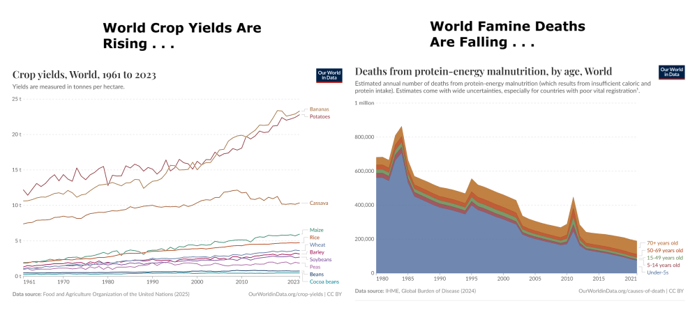
Dire predictions are often based on flawed models, exaggerations, wild imaginations and a failure to factor in human ingenuity.335 Predictions made in the 1970s of an impending ice age, falling crop yields, increasing global famine, advancing deserts, a pesticide-induced cancer epidemic, of oil, gas and other resources rapidly running out, were not only wrong but the very opposite has happened.

More recent predictions of malaria spreading across the globe, Arctic ice disappearing by 2013, increasing droughts and tropical cyclones have all failed to materialize. Indeed, the world has never been safer than now (Fig. 30).

The academic left first quarreled with science339 before capturing, corrupting and politicizing it. They then ignored quantitative uncertainties343 to contrive a catastrophic climate change consensus, calling sceptics deniers and inventing a climate crisis and global boiling to foster fear, funding and a rush to renewables. Anthropocentric purists prohibit alternative diagnoses, prognoses, priorities or remedies and suspect fossil fuel funding behind anyone challenging “The Science”. Climate change does impact the poorest the most but, as we shall see in the next section, a lucrative climate industry makes them even poorer and more vulnerable.

Conclusion

Warmth is good for human health and prosperity. Fossil fuels have played a vital role in providing the wealth essential for health and environmental protection. They have also boosted atmospheric CO2 and added a little warmth, both being hitherto beneficial overall for plants and people. The ingenuity of Homo sapiens at adapting to climate has permitted people to populate almost the entire globe from the freezing Arctic to the steamy tropics. If we stick to doing what we do best – adaptation – we will continue to thrive.

We must be prepared not only for global warming, but also for global cooling,
which will surely occur as our present warm Holocene draws to its inevitable end.

Human health and that of the planet depends on balancing productivity and development with conservation and environmental protection. Only developed countries with people lifted out of poverty can afford to produce clean energy, protect the environment, put power lines underground, construct buildings with 5-star energy ratings and use efficient lighting/appliances to minimize energy and water use, provide adequate safe water supplies and effective public health measures to control communicable diseases. It is vital that governments focus on real pollutants, not imagined ones, and that they avoid using climate change as a scapegoat for failure to implement sound public health policies and proven preventive measures. Misguided climate action can be worse than unmitigated climate change.

The 2014 IPCC Summary for Policymakers nicely summed it up:

“The most effective vulnerability reduction measures for health in the near term are programs that implement and improve basic public health measures such as provision of clean water and sanitation, secure essential health care including vaccination and child health services, increase capacity for disaster preparedness and response, and alleviate poverty (very high confidence).”


No Right to Stable Climate in Our Holocene Epoch

Leszek Marks explains how warming and cooling alternated throughout the last 12,000 years and how our modern period is no different in his paper Contemporary global warming versus climate change in the Holocene.  Excerpts in italics with my bolds and added images.  H/T No Tricks Zone

Leszek Eugeniusz Marks is a Polish geologist, professor ordinarius, currently at the Warsaw University, Department of Climate Geology; and the Polish Geological Institute-National Research Institute, president of Committee for Quaternary Research of the Polish Academy of Sciences. At present, member of editorial boards of scientific journals Boreas, “Litosfera”, “Geography and Geology”, and Studia Quaternaria.

Abstract

Cyclical climate change is characteristic of the Holocene, with successive warmings and coolings. A solar forcing mechanism has steered Holocene climate change, expressed by 9 cooling phases known as Bond events. There is reliable geological evidence that the temperatures of most warming phases in the Holocene were globally higher or similar to that of the current warming period, Arctic sea ice was less extensive and most mountain glaciers in the northern hemisphere either disappeared or were smaller.
During the African Humid Period in the Early and Middle Holocene, much stronger summer monsoons made the Sahara green with growth of savanna vegetation, huge lakes and extensive peat bogs. The modern warming is part of a climatic cycle with a progressive warming after the Little Ice Age, the last cold episode of which occurred at the beginning of the 19th century. Successive climate projections of the Intergovernmental Panel on Climate Change are based on the assumption that the modern temperature rise is steered exclusively by the increasing content of human-induced CO2 in the atmosphere. If compared with the observational data, these projected temperatures have been highly overestimated.

Overview

This paper presents the current state of knowledge of the climate change in the Holocene. The geological record of the climate change in this epoch has been verified by the results of archaeological, historical and meteorological investigations (Marks, 2016). Determination of the steering forces of modern warming is among the current scientific priorities in the world and, therefore, geological input is an important contribution to the discussion about human impact on the climate.

The current interglacial of the Holocene started 11.7 ka cal BP (Walker et al., 2018), with progressively increasing human impact on the Earth’s environment, especially strong during the past decades (Gibbard et al., 2021). Geological examination of past climate changes is crucial to distinguish the natural and the human-induced factors of the current climate change. The most important climate-steering factor is solar radiation, subjected to cyclical changes caused by the Sun’s activity that supplies with over 99% of the energy that is responsible for the climate of the Earth. Geological reconstructions show that rises and falls in the temperature on the Earth are dependent on the sunspot cycles (Table 1; Easterbrook, 2011; Usoskin et al., 2016; Usoskin,2023), and these in turn respond to the varying magnetic activity of the Sun.

The natural input of solar energy is transformed by different external and internal factors to modulate climate on the Earth. Latitudinal insolation in the Holocene depended on the Earth’s orbital parameters (Milankovič cycles). In comparison with the present values, summer temperatures in the northern hemisphere were higher in the Early and Middle Holocene (Beer, Van Geel, 2008; Beer, Wanner, 2012). Winter temperatures in the southern hemisphere were higher in the Middle Holocene, followed by higher temperatures in the northern hemisphere in the Late Holocene. In the coming 3 ka, lower temperatures are expected everywhere, except for the intertropical zone where higher winter temperatures are expected (Marks, 2016).

The natural rhythm of climate change during the Holocene was disturbed by large volcanic eruptions. Emission of dust into the atmosphere was responsible for a couple of cold events during the Holocene (Shindell et al., 2003). Such eruptions can be detected by concentrations of SO2 in polar ice core records (Zielinski et al., 1994; Castellano et al., 2004). The extent of the vegetation cover had an important, but very complex, effect on the climate (Foley et al., 2003), because the evaporative cooling by a forest mitigated warmings and limited dust mobilisation (Bonan, 2008). The atmospheric CO2 concentration decreased in the Early Holocene and started to increase since 7 ka, being independent of temperature variations (Palacios et al., 2024a). Ocean-atmosphere interchange was the main source of CO2 until the recent decades when the anthropogenic emission of CO2 became significant (Brovkin et al., 2019).

Fig. 1. Climate change in the Holocene, adapted from Palacios et al. (2024a) and modified: warm periods are in yellow and less warm in pale yellow, and cold in blue; Bond Events are after Bond et al. (1997, 2001) and geochronology after Walker et al. (2019).

Climate change after the Holocene Thermal Maximum

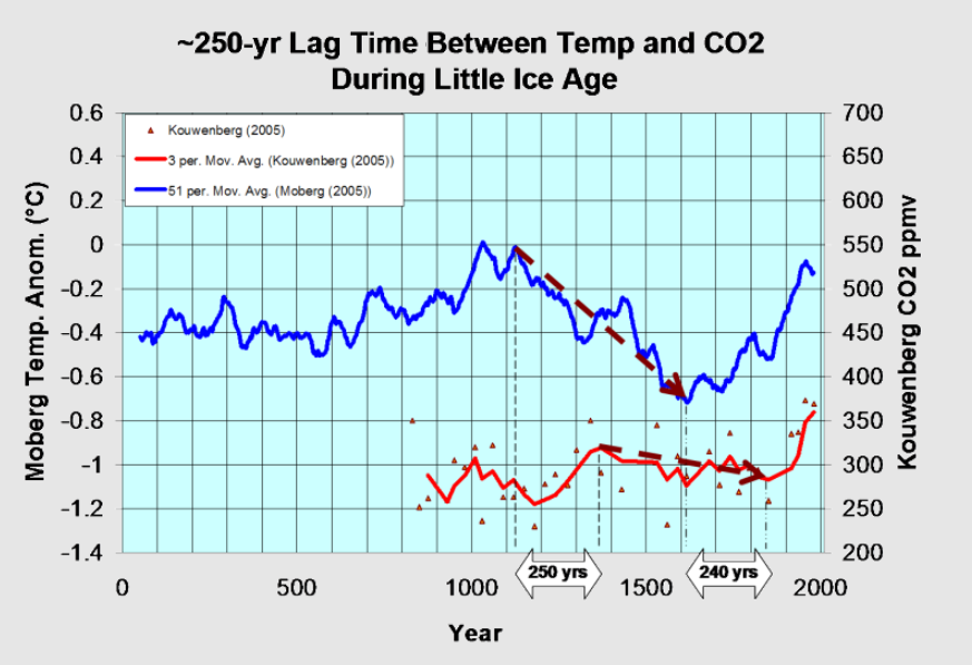
The temperature deduced from the oxygen isotope curve in the Greenland ice core GISP2 shows that several warmings occurred after the Holocene Thermal Maximum (Fig. 1; Drake, 2012). These were periods during which great progress in the development of human societies occurred: Late Bronze Age, Roman Warm Period and the MWP.  The separating cold Bond Events, named the Iron Age and Dark Ages Cold Periods respectively, were expressed by economic, intellectual and cultural decline. The temperature history since 900 CE was based firstly on the estimated climate history of central England (Lamb, 1977; IPCC, 1990). This showed a distinct warming of ~1.3°C when compared with the LIA (Moberg et al., 2005; D’Arrigo et al., 2006; Mann et al., 2009). This warming was a result of natural processes, because human activity could not have had any significant effect on temperature changes before 1900 CE. The Roman Warm Period (250 BC–450 CE), the MWP (950–1250 CE) and the Modern Warming Period reflect 1000-cycles with high solar radiation (Table 1; Vahrenholt, Lüning, 2014).

Discussion

The claim of the IPCC (2021) that ‘…the latest decade was warmer than any multi-century period after the Last Interglacial, around 125,000 years ago’ ignores all the knowledge about reconstructed temperatures in the Holocene, based on multi-proxy palaeoclimatic data.

Despite the extensive northern ice sheets, the increased summer insolation in the northern hemisphere caused a warming trend from the beginning of the Holocene and lasting until the Middle Holocene (Palacios et al., 2024a).  This warming trend was reversed from 6–5 ka onwards, due to decreased summer insolation in the northern hemisphere. Such general warming or cooling trends in the Holocene were interrupted by short periods with opposite and abrupt temperature changes (Fig. 1).

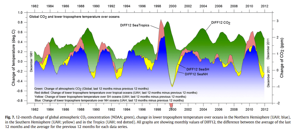
The modern warming represents a part of the cyclical climate change after the LIA, the last cold episode of which occurred at the beginning of the 19th century. The LIA with low temperatures is named the pre industrial period by the advocates of global anthropogenic warming and such an approach helps them to promote the idea that an increased human emission of CO2 (especially in the 20th century) is the only reason for rising temperatures on Earth. They do not bother with the evidence that the mutual time relations of global temperature and contents of CO2 in the atmosphere in 1980–2019 indicate a leading role of temperature, a rise of which was followed in that time by a 6-month delay in the rise of CO2 (Humlum et al., 2012; Koutsoyiannis, Kundzewicz, 2020).

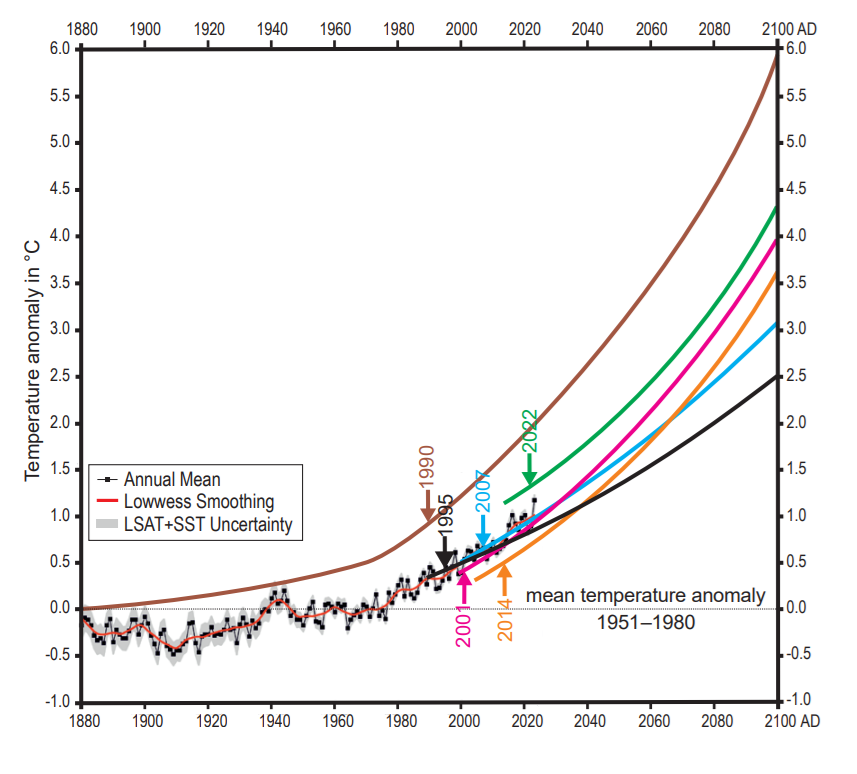
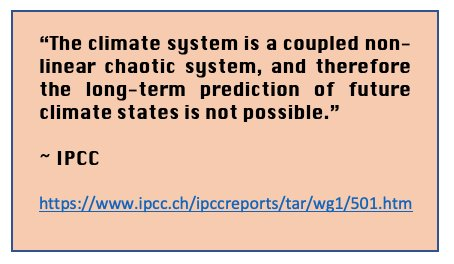
The official curve of the global mean annual temperature anomalies based on regular measurements (https://data.giss.nasa.gov/gistemp/graphs_v4/) overlaps slightly with the temperature projections in reports of the IPCC (1990, 1995, 2001, 2007, 2014, 2021). These IPCC projections were created by climate models, based on the assumption that the modern temperature rise is steered exclusively by the increasing content of human-induced CO2 in the atmosphere while the role of water vapour as the main greenhouse gas is neglected (cf. Hołyst, 2020). Such an approach makes the IPCC-projected temperature highly overestimated if compared with the observational data (Fig. 3). Despite the lockdowns during the Covid-19 pandemic in 2020–2021, connected with large cutbacks in transport, travel, industrial production and energy generation, no reduction in atmospheric CO2 was noted. This fact suggests that the proposed reductions in global energy use would be most probably highly ineffective in limiting the level of atmospheric CO2.

Fig. 3. Global estimates of mean annual temperature anomalies (1880–2023), based on land and ocean data (https://data.giss.nasa.gov/gistemp/graphs_v4/) and temperature projections to AD 2100 in the successive IPCC reports (1990, 1995, 2001, 2007, 2014, 2021)

Conclusions

The Holocene climate change was characterized by cyclical warmings (such as: Holocene Thermal Maximum, Late Bronze Age, Roman Warm Period, MWP) and coolings (Bond Events: including Iron Age Cold Period, Dark Ages Cold Period and LIA). The IPCC claims that current warming is unprecedented in the last 2000 or even the last 125,000 years; this statement is very unconvincing and it is not supported by the geological data. There is good evidence that both in the last 2000 years as well during the Holocene Thermal Maximum, temperatures were higher or broadly similar to the ones in the current warming period, the Arctic sea ice was less extensive and most mountain glaciers (especially in the northern hemisphere) either disappeared or were smaller. Much stronger summer monsoons in the Early and Middle Holocene made the Sahara green with savanna vegetation, huge lakes and extensive peat bogs. The terms ‘the Holocene Thermal Maximum’ and ‘the Holocene Climatic Optimum’ are avoided by the IPCC (2021), and its popularized statements making the current warming look ‘unprecedented’ and therefore ‘unique’ are false and flatten the climate history (cf. Marcott et al., 2013).

The climate is a product of complicated interdependence of many factors that have not been yet sufficiently recognized qualitatively and quantitatively. It is a great scientific challenge that requires an extensive interdisciplinary research. There is a crucial need to make climate science less political and climate policy more scientific.


The Fracking Truth

Linnea Lueken sers the record straight on fracking in the above video from Prager U.  Transcript in italics below with my added images.

It is one of the greatest innovations of the last fifty years.

It has saved consumers billions of dollars…

Prevented untold tons of carbon emissions from entering the atmosphere…

And almost single-handedly rescued an economy that was in the middle of a severe downturn.

You’ve probably heard of this innovation — not as a source of pride, but as an object of scorn.

I’m talking about fracking: the process of extracting oil and natural gas from fine cracks in shale rock.

So, what gives?

Originated from treehugger.com

Why has something that has done so much good been so unappreciated — even vilified?

The answer, of course, is that the opponents of fracking — environmentalists and their political and media allies — say that the negatives of fracking outweigh its positives.

What are those negatives?

Detractors have a long list: contributing to global warming, putting local drinking water at risk, and even causing earthquakes are high among their complaints.

Those are pretty serious charges. But are they valid?

Before I answer that question, let’s cover a little history.

Fracking — whatever your current impression of it — is a great American success story.

Before the twenty-first century, fracking as we know it now barely existed. The concept — reaching pockets of oil and gas trapped in shale — had been around for decades, but wasn’t practically or financially feasible.

Technological breakthroughs and a few eureka moments — like horizontal drilling and using improved ground-penetrating radar — in the early 2000s changed everything.

In traditional oil production, a company drills a well with the goal of finding a reservoir of oil. In fracking, the goal is to liberate a vast number of small pockets of oil and gas that have been trapped in the shale rock.

A narrow shaft is drilled — first vertically, and then horizontally. Water, mixed with sand and other additives, is pumped down the shaft at extremely high pressure to create tiny fissures in the surrounding rock. The sand holds the tiny cracks open, allowing the oil and gas to escape and flow back up the well to the surface.

What makes the innovation of fracking even more remarkable is that it emerged at a time when the theory of “Peak Oil” was widely accepted. Advocates of this theory—including many prominent scientists—warned that humans would soon run out of fossil fuels.

Fracking turned the theory upside down. In a matter of a few years, the world had more oil and gas than it knew what to do with — most of it coming from the United States.

The benefits from the fracking revolution were almost immediate.

The price of natural gas fell from $9 per cubic foot to $3. Consumers saved big on their gas and electric bills.

As gas replaced coal as a cheap, reliable energy source, greenhouse gas emissions fell more than 20%.

The US economy, reeling from the 2008 financial crisis, reversed course. The fracking boom was the number one reason.

Ironically, the politician who benefited the most from this boom was a fierce foe of fossil fuels, President Barack Obama. And, while he continued to push his green agenda, he did almost nothing to stop the fracking phenomenon.

Perhaps he read the science. It emphatically endorses natural gas as a clean energy source. Even Carl Pope, then the executive director of the Sierra Club, one of the world’s largest environmental groups, came out for fracking. As Pope saw it, natural gas was the perfect transition between fossil fuels and alternative energy.

With that history in mind, let’s return to the charges made by opponents of fracking.

The EPA — hardly a friend of the oil and gas industry — has looked closely into the question of whether fracking puts aquifers, the source of much of our drinking water, at risk. One EPA study examined 110,000 fracking sites. It concluded that fracking does not pose a threat. One obvious reason is that fracking is done at depths of six to ten thousand feet. Water tables tend to be at 500 feet or higher.

What about the concern that fracking causes earthquakes? Numerous studies have concluded that related tremors are so minor they’re barely detectable and cause no damage. At its worst, it produces vibrations comparable to a passing truck.

VibratAir pollution?

According to the EPA emissions of sulfur, nitrogen, mercury, particulates, and carbon dioxide have all declined since large-scale fracking began and natural gas replaced coal for much of the nation’s electricity production.

Something else that natural gas has going for it which isn’t talked about much is land use. Per megawatt, natural gas uses about 12.4 total acres – including mining and transmission lines. By comparison, solar uses about 43.5 acres per megawatt, and wind uses more than 70.

More energy, less pollution, lower prices for consumers, small footprint.

Instead of vilifying fracking, maybe we should throw it a parade.

I’m Linnea Lueken, research fellow at the Heartland Institute, for Prager University.

New England Facing Energy Crisis, Worries About Bugs

Linnea Lueken explains the false alarm in her Climate Realism article Climate Change Is Not Causing New England’s ‘Creepy’ Bacteria and Bugs, Boston Globe.  Excerpts in italics with my bolds and added images.

The Boston Globe posted an article titled “Climate change is bringing creepy — and dangerous — bacteria, bugs, and viruses to New England,” claiming that global warming is “fueling an increase in bacteria and disease” in New England. The headline and the attached story are highly misleading. For things like mosquito-borne illness, mosquitos carrying diseases previously thrived even in New England in previous centuries, with 20th century human intervention wiping them out, not temperature changes. Also, bacteria in waterways are a seasonal phenomenon which has always existed.

The Real New England Crisis is Green Agenda Attack on Electricity Supply

Source: granitegeek, Concord Monitor

Daniel Turner explains in his Real Clear Energy article The Green Agenda Turned New England Into an Energy Price Punchline.  Excerpts in italics with my bolds and added images.

Fall is here, the leaves are changing, the temperature is dropping and sadly New England families know the routine.

Every month, the electric bill arrives, and it’s larger than the month before. The region pays more for electricity than almost anyone else in America—higher than the national average and, outside of Alaska and Hawaii, higher than anywhere else in the country. This is not a coincidence. It is the inevitable result of politicians who pushed the risky and unreliable green agenda while forcing reliable power plants off the grid.

Here’s an inconvenient history lesson. When Joe Biden took office, electricity in New England cost 20.7 cents per kilowatt-hour. By the time he left, it was more than 28.2 cents. That’s a staggering spike of more than 36% in just four years. Hundreds of dollars gone from family budgets and small businesses every single year. For working households already feeling the squeeze of Biden’s inflation, it can mean the difference between savings and debt, between heating a home and keeping it uncomfortably cold.

October 2022 generation in New England, by fuel source

And the blame is clear. The forced closure of coal, oil, and natural gas plants in the name of “climate progress” is why rates are climbing. In 2022, Massachusetts Senators Elizabeth Warren and Ed Markey traveled to Somerset to celebrate the shutdown of traditional energy plants. They smiled for the cameras, congratulated themselves on a “victory,” and then went back to Washington while families were left to pay the tab.

First came the celebration, but now we see the deflection. Four Democratic senators, including Warren and Markey, recently wrote a letter to the Trump administration suddenly pretending to care about rising electricity bills. It is political theater and nothing more. They didn’t care when they cheered the closures in 2022, and they don’t care now. New England’s families are stuck with the consequences of the green agenda they applauded; they just want to escape the blame.

Project abandoned in 2017 after New York blocked planning and permit processes.

Let’s be clear: This cascade of closures started when Joe Biden was vice president and accelerated under his presidency. Nearly 400 fossil fuel plants have been shuttered across the country since 2010, including almost 300 coal plants. In the Northeast alone, names like Indian Point in New York, Eagle Point in New Jersey, Schiller Station in New Hampshire, and Canal Station in Massachusetts have been crossed off the map. Each closure meant fewer megawatts of reliable power and higher bills for families.

 Project abandoned in April 2016

The problem is not complicated. Shutting down affordable, always-on power and replacing it with expensive, intermittent sources like wind and solar leads to higher prices. Add the surge in demand from artificial intelligence data centers, which analysts say could double electricity consumption by 2030, and the consequences are obvious: higher costs, weaker reliability, and a grid at the breaking point.

There is a way out of this crisis, but it requires real action, not pointless blaming. My organization, Power The Future, lays out the steps in our recent report.

♦  First, use the Defense Production Act to treat grid reliability as the national security issue it is, and direct resources to keep critical plants online.
♦  Second, build new fossil fuel plants—modern natural gas and coal facilities that can deliver decades of dependable, affordable power.
♦  Third, halt premature closures until replacement capacity is running, not just promised on paper. And fourth, expand the capacity of existing coal plants, many of which are running below potential thanks to political limits, to quickly add thousands of megawatts back to the grid.

These are not radical ideas. They are common sense. They put working families, not political slogans, at the center of energy policy. They recognize that you cannot run a 21st-century economy on wishful thinking, photo-ops, and subsidies for technology that fails when the wind doesn’t blow, or the sun doesn’t shine.

Too many of New England’s “leaders” in Washington have turned their states into punchlines of America’s power prices. Working families deserve leaders who care more about their constituents’ bills than their standing with environmental activists. They deserve an energy policy grounded in reality, not ideology.

If you want to know who killed affordable power in New England, it wasn’t President Trump and it wasn’t the utility companies. All you need to do is just look at who popped the champagne when the plants closed.


Climate Lawsuits in Montana

Ed Berry provides an update and background on climate lawfare in his home state.

There have been three climate lawsuits in Montana from Our children’s Trust:

  1.  Barhaugh v Montana in 2011.
  2.  Held v Montana in 2022-2023.
  3.  Lighthiser v Trump in 2025.

There has been little change in the wording of these climate lawsuits. HvM still has AG Bullock’s name in it even though Montana elected him Governor as of 2012. The science argument in these three climate lawsuits has not changed.

They all claim the government is damaging the physical and mental health of children by allowing human CO2 emissions to continue.

But the schools and parents are damaging their children’s mental and health brainwashing them to believe human carbon emissions are destroying the planet.

The fundamental science issue in all climate lawsuits is whether these unstated hypotheses are true or false:

(1)   Human CO2 causes all the CO2 increase above 280 ppm.

(2)   This CO2 increase causes global warming.

(3)   This global warming causes the plaintiffs claimed damages.

The plaintiffs assume these three hypotheses are true, and they will admit it in court. Otherwise, they would have no basis for their claims.

To prevail, the defense needs to prove only one of these hypotheses is false. In fact, it is easy to prove all three hypotheses are false in a court of law.

Here’s a critical point that few people understand:

The scientific method says it is impossible to prove a hypothesis is true so the alarmists cannot prove these hypotheses are true. The plaintiffs have the burden of proof.

However, we can prove these hypotheses are false by showing they make one false prediction or contradiction with data. This is the key to science.

This is what parents and teachers and media should be teaching the kids.

1.      Barhaugh v. Montana

Barhaugh v. Montana: Petition for Original Jurisdiction, Montana Supreme Court, 2011, was the first climate lawsuit in Montana.

To justify its petition to the Montana Supreme Court, BvM says on page 5:

  • Through the normal litigation and appeals process, this issue would likely take a minimum of two to three years just to reach this Court, in contrast to the average 60 days needed to resolve original proceedings.
  • “Considering the scientific evidence cited by the Respondent, there is not enough time to effectively arrest the effect of human-caused climate change unless immediate action is taken.”
  • “Climatological “tipping points” lie directly ahead and drive the urgency of taking action:
  • The further we look into the future, the worse the costs of inaction will become. The longer we do nothing, the greater the risks of an irreversible climate catastrophe, such as a massive rise in sea levels, which could make the world unable to support anything like the current levels of population and economic activity. The costs and risks of inaction are overwhelmingly worse than the moderate and manageable costs of an immediate effort to reduce carbon emissions.”

Barhaugh v. Montana justified its petition to the Montana Supreme Court by predicting an irreversible climatological “tipping point” would occur in the next three years.

The Petition is based upon its assumption that the three unstated climate hypotheses are true. Assuming these hypotheses are true, the plaintiffs claimed certain damages. But all their claims are based on their assumption that their three hypotheses above are true.

The Intervention led by Dr. Edwin X Berry of Bigfork, Montana, prevented the Montana Supreme Court from ruling in favor of the Petition.

Berry’s Intervenors presented evidence that contradicted the Petition’s assumptions.

Their evidence constrained Montana Attorney General Bullock’s reply to the Court because he could not go on record disputing the Intervenors’ evidence that the Petitioners’ claims about climate science may not be true.

Montana AG Bullock wrote:

  • This disputed record is just one example of the factual determinations this Court would need to make to rule for Petitioners.
  • In addition, it would need to address, among other issues, the current state of climate change science; the role of Montana in the global problem of climate change; how emissions created in Montana ultimately affect Montana’s climate; whether the benefits of energy production must be balanced against the potential harm of climate change; and the concrete limits, if any, of the alleged “affirmative duty.”

The Montana Supreme Court ruled:

  • As the State points out, the petition incorporates factual claims such as that the State “has been prevented by the Legislature from taking any action to regulate [greenhouse gas] emissions.”
  • The State posits that the relief requested by Petitioners would require numerous other factual determinations, such as the role of Montana in the global problem of climate change and how emissions created in Montana ultimately affect Montana’s climate.
  • This Court is ill-equipped to resolve the factual assertions presented by Petitioners. We further conclude that Petitioners have not established urgency or emergency factors that would preclude litigation in a trial court followed by the normal appeal process.

The court could not determine whether the Petitioners or the Intervenors were correct about climate because, in the court’s view, there is no scientific consensus that is sufficiently well-settled to decide the case as a matter of law.

The Court rejected the Barhaugh v. Montana Petition.

Quentin Rhoades, Attorney for the Intervenors, wrote that the Montana Supreme Court ruled against the Petitioners because,

  • “There is no scientific consensus that is sufficiently well-settled to allow a court to decide the case purely as a matter of law.

Rhoades concluded,

  • This establishes once and for all, at least as far as Montana law is concerned, climate science is decidedly not settled.
  • “And not only is it the highest court of a sovereign state, but it ruled that there is no scientific consensus that is sufficiently well-settled to allow for them to decide the case purely as a matter of law.” 

2.      Held v Montana

Montana AG Knudsen should have dismissed Held v Montana based on the now-proven-false climate prediction of Barhaugh v. Montana and the Montana Supreme Court ruling.

The Montana Supreme Court ruled in 2011,

  • “There is no scientific consensus that is sufficiently well-settled to allow a court to decide the case purely as a matter of law.”

Consensus has no bearing on scientific truth. Montana’s AG Knudsen should have known this because all trial lawyers learn it.

Republican AG Knudson should have argued that consensus proves nothing in science. The only relevant proof in science is proof that a hypothesis is false.

Yet AG Knudsen stipulated “consensus” was valid at the beginning of the HvM trial:

  • for the purposes of trial, there is a scientific consensus that earth is warming as a direct result of human GHG emissions, primarily from the burning of fossil fuels.”

AG Knudsen’s “consensus” stipulation contradicted the Montana Supreme Court.

AG Knudsen’s climate stipulation put him to the left of former Democrat AG Bullock.

On 9/16/2025, Matthew Brown, of the lying Associated Press, wrote about HvM:

  • Young climate activists and their attorneys who won a landmark global warming trial against the state of Montana are trying to convince a federal judge to block President Donald Trump’s executive orders promoting fossil fuels.

No, they did not “win.” Montana AG Knudsen purposely LOST Held v Montana as Montana WEF man ordered him to do.

Knudsen produced NO defense, NO relevant expert witness, and NO challenge to the plaintiffs’ expert witness claims. He laid on the grass and let the opposition trample on Montana.

Knudsen’s purposeful loss of HvM is the worst betrayal by an elected official of the people who voted for him that I have ever witnessed.

3.    Lighthiser v Trump

Lighthiser v. Trump uses the same bad science as Barhaugh v. Montana and Held v Montana.

On September 17, 2025, I traveled to Missoula and sat in on part of the Lighthiser v Trump trial. In my view, Trump’s attorney made good arguments to dismiss LvT. Now, we wait for the judge to decide whether to dismiss LvT.

If LvT continues, I encourage Trump’s attorney to use the arguments that I describe in my other articles to prove hypotheses (1), (2), and (3) are false. They are easy proofs to make in court.

If the LvT trial continues, Trump’s attorney should plan to prove hypotheses (1) and (2) are false and as a bonus prove that (3) is also false. This defeat would remove the influence of the climate fraud on politics.

Comment:

September 17 and 18, 2025, was a two-day injunction hearing in the case of Lighthiser v. Trump, in the Federal District of Montana Butte Division.  While federal Judge Dana Christensen listened to a few more of the plaintiffs’ witnesses and closing arguments, he was mulling over a few difficult legal questions regarding the plaintiffs’ injunction request. [Source: Missoula Current]

“In your motion, it says you want a preliminary injunction from me prohibiting the defendants from implementing these three orders. What exactly does that look like? I enjoin them, and what else do I do?” Christensen asked plaintiffs’ attorney Julia Olson during her closing statement. “Let’s assume these defendants elect to continue to implement policy favoring fossil fuels regardless of what I say. What will I do then?”

Olson said the defense attorneys hadn’t contested the statement that the central purpose of the executive orders is unleashing fossil fuels. But in his closing statement for the defense, DOJ attorney Michael Sawyer said that wasn’t the only thing the plaintiffs had to show. They have to prove they have standing by showing how they’re harmed by the executive orders and how that harm might be relieved by an injunction and eventually a ruling. That last part, known as redressability, was perplexing Christensen, and Sawyer weighed in, saying such an “unprecedented” injunction would be too difficult to police.

“If there were to be a preliminary injunction, there would be numerous requests back here. Every time an agency action is issued that plaintiffs didn’t like, that they thought was too friendly to fossil fuels, they’d be back here again,” Sawyer said. “What we have here is hundreds of lawsuits packed into one.”

The Defendants Brief in Opposition to Plantiffs’ Motion for Preliminary Injunction is here.

In addition to the AG Montana and US DOJ, the submission was joined by AGs from:

Alaska, Arkansas, Florida, Georgia, Idaho, Indiana, Iowa, Kansas, Louisiana, Missouri, Nebraska, North Dakota, Oklahoma, South Dakota, Texas, Utah, West Virginia, Wyoming, and Guam


August 2025 Ocean SSTs: NH Warms Slightly

The best context for understanding decadal temperature changes comes from the world’s sea surface temperatures (SST), for several reasons:

  • The ocean covers 71% of the globe and drives average temperatures;
  • SSTs have a constant water content, (unlike air temperatures), so give a better reading of heat content variations;
  • A major El Nino was the dominant climate feature in recent years.

Previously I used HadSST3 for these reports, but Hadley Centre has made HadSST4 the priority, and v.3 will no longer be updated. I’ve grown weary of waiting each month for HadSST4 updates, so this report is based on data from OISST2.1.  This dataset uses the same in situ sources as HadSST along with satellite indicators.  Importantly, it produces daily anomalies from baseline period 1991-2020.  The data is available at Climate Reanalyzer (here).  Product guide is (here).  The charts and analysis below is produced from the current data.

The Current Context

The chart below shows SST monthly anomalies as reported in OISST2.1 starting in 2015 through August 2025. A global cooling pattern is seen clearly in the Tropics since its peak in 2016, joined by NH and SH cycling downward since 2016, followed by rising temperatures in 2023 and 2024 and cooling in 2025.

Note that in 2015-2016 the Tropics and SH peaked in between two summer NH spikes.  That pattern repeated in 2019-2020 with a lesser Tropics peak and SH bump, but with higher NH spikes. By end of 2020, cooler SSTs in all regions took the Global anomaly well below the mean for this period.  A small warming was driven by NH summer peaks in 2021-22, but offset by cooling in SH and the tropics, By January 2023 the global anomaly was again below the mean.

Then in 2023-24 came an event resembling 2015-16 with a Tropical spike and two NH spikes alongside, all higher than 2015-16. There was also a coinciding rise in SH, and the Global anomaly was pulled up to 0.6°C in 2023, ~0.2° higher than the 2015 peak.  Then NH started down autumn 2023, followed by Tropics and SH descending 2024 to the present. During 2 years of cooling in SH and the Tropics, the Global anomaly came back down, led by Tropics cooling the last 12 months from its 0.9°C peak last August, down to 0.3C in August this year. Small changes in NH and SH offset each other, leaving the global anomaly the same.

Comment:

The climatists have seized on this unusual warming as proof their Zero Carbon agenda is needed, without addressing how impossible it would be for CO2 warming the air to raise ocean temperatures.  It is the ocean that warms the air, not the other way around.  Recently Steven Koonin had this to say about the phonomenon confirmed in the graph above:

El Nino is a phenomenon in the climate system that happens once every four or five years.  Heat builds up in the equatorial Pacific to the west of Indonesia and so on.  Then when enough of it builds up it surges across the Pacific and changes the currents and the winds.  As it surges toward South America it was discovered and named in the 19th century  It iswell understood at this point that the phenomenon has nothing to do with CO2.

Now people talk about changes in that phenomena as a result of CO2 but it’s there in the climate system already and when it happens it influences weather all over the world.   We feel it when it gets rainier in Southern California for example.  So for the last 3 years we have been in the opposite of an El Nino, a La Nina, part of the reason people think the West Coast has been in drought.

It has now shifted in the last months to an El Nino condition that warms the globe and is thought to contribute to this Spike we have seen. But there are other contributions as well.  One of the most surprising ones is that back in January of 2022 an enormous underwater volcano went off in Tonga and it put up a lot of water vapor into the upper atmosphere. It increased the upper atmosphere of water vapor by about 10 percent, and that’s a warming effect, and it may be that is contributing to why the spike is so high.

A longer view of SSTs

To enlarge, open image in new tab.

The graph above is noisy, but the density is needed to see the seasonal patterns in the oceanic fluctuations.  Previous posts focused on the rise and fall of the last El Nino starting in 2015.  This post adds a longer view, encompassing the significant 1998 El Nino and since.  The color schemes are retained for Global, Tropics, NH and SH anomalies.  Despite the longer time frame, I have kept the monthly data (rather than yearly averages) because of interesting shifts between January and July. 1995 is a reasonable (ENSO neutral) starting point prior to the first El Nino.

The sharp Tropical rise peaking in 1998 is dominant in the record, starting Jan. ’97 to pull up SSTs uniformly before returning to the same level Jan. ’99. There were strong cool periods before and after the 1998 El Nino event. Then SSTs in all regions returned to the mean in 2001-2.

SSTS fluctuate around the mean until 2007, when another, smaller ENSO event occurs. There is cooling 2007-8,  a lower peak warming in 2009-10, following by cooling in 2011-12.  Again SSTs are average 2013-14.

Now a different pattern appears.  The Tropics cooled sharply to Jan 11, then rise steadily for 4 years to Jan 15, at which point the most recent major El Nino takes off.  But this time in contrast to ’97-’99, the Northern Hemisphere produces peaks every summer pulling up the Global average.  In fact, these NH peaks appear every July starting in 2003, growing stronger to produce 3 massive highs in 2014, 15 and 16.  NH July 2017 was only slightly lower, and a fifth NH peak still lower in Sept. 2018.

The highest summer NH peaks came in 2019 and 2020, only this time the Tropics and SH were offsetting rather adding to the warming. (Note: these are high anomalies on top of the highest absolute temps in the NH.)  Since 2014 SH has played a moderating role, offsetting the NH warming pulses. After September 2020 temps dropped off down until February 2021.  In 2021-22 there were again summer NH spikes, but in 2022 moderated first by cooling Tropics and SH SSTs, then in October to January 2023 by deeper cooling in NH and Tropics.

Then in 2023 the Tropics flipped from below to well above average, while NH produced a summer peak extending into September higher than any previous year.  Despite El Nino driving the Tropics January 2024 anomaly higher than 1998 and 2016 peaks, following months cooled in all regions, and the Tropics continued cooling in April, May and June along with SH dropping.  After July and August NH warming again pulled the global anomaly higher, September through January 2025 resumed cooling in all regions, continuing February through April 2025, with little change in May,June and July despite upward bumps in NH.

What to make of all this? The patterns suggest that in addition to El Ninos in the Pacific driving the Tropic SSTs, something else is going on in the NH.  The obvious culprit is the North Atlantic, since I have seen this sort of pulsing before.  After reading some papers by David Dilley, I confirmed his observation of Atlantic pulses into the Arctic every 8 to 10 years.

Contemporary AMO Observations

Through January 2023 I depended on the Kaplan AMO Index (not smoothed, not detrended) for N. Atlantic observations. But it is no longer being updated, and NOAA says they don’t know its future.  So I find that ERSSTv5 AMO dataset has current data.  It differs from Kaplan, which reported average absolute temps measured in N. Atlantic.  “ERSST5 AMO  follows Trenberth and Shea (2006) proposal to use the NA region EQ-60°N, 0°-80°W and subtract the global rise of SST 60°S-60°N to obtain a measure of the internal variability, arguing that the effect of external forcing on the North Atlantic should be similar to the effect on the other oceans.”  So the values represent SST anomaly differences between the N. Atlantic and the Global ocean.

The chart above confirms what Kaplan also showed.  As August is the hottest month for the N. Atlantic, its variability, high and low, drives the annual results for this basin.  Note also the peaks in 2010, lows after 2014, and a rise in 2021. Then in 2023 the peak reached 1.4C before declining to 0.9 last month.  An annual chart below is informative:

Note the difference between blue/green years, beige/brown, and purple/red years.  2010, 2021, 2022 all peaked strongly in August or September.  1998 and 2007 were mildly warm.  2016 and 2018 were matching or cooler than the global average.  2023 started out slightly warm, then rose steadily to an  extraordinary peak in July.  August to October were only slightly lower, but by December cooled by ~0.4C.

Then in 2024 the AMO anomaly started higher than any previous year, then leveled off for two months declining slightly into April.  Remarkably, May showed an upward leap putting this on a higher track than 2023, and rising slightly higher in June.  In July, August and September 2024 the anomaly declined, and despite a small rise in October, ended close to where it began.  Note 2025 started much lower than the previous year and headed sharply downward, well below the previous two years, then since April through August aligning with 2010.

The pattern suggests the ocean may be demonstrating a stairstep pattern like that we have also seen in HadCRUT4.

The rose line is the average anomaly 1982-1996 inclusive, value -0.25.  The orange line the average 1982-2025, value -0.014 also for the period 1997-2012. The red line is 2015-2025, value 0.32. As noted above, these rising stages are driven by the combined warming in the Tropics and NH, including both Pacific and Atlantic basins.

Curiosity:  Solar Coincidence?

The news about our current solar cycle 25 is that the solar activity is hitting peak numbers now and higher  than expected 1-2 years in the future.  As livescience put it:  Solar maximum could hit us harder and sooner than we thought. How dangerous will the sun’s chaotic peak be?  Some charts from spaceweatherlive look familar to these sea surface temperature charts.

Summary

The oceans are driving the warming this century.  SSTs took a step up with the 1998 El Nino and have stayed there with help from the North Atlantic, and more recently the Pacific northern “Blob.”  The ocean surfaces are releasing a lot of energy, warming the air, but eventually will have a cooling effect.  The decline after 1937 was rapid by comparison, so one wonders: How long can the oceans keep this up? And is the sun adding forcing to this process?

uss-pearl-harbor-deploys-global-drifter-buoys-in-pacific-ocean

USS Pearl Harbor deploys Global Drifter Buoys in Pacific Ocean

Tropics UAH Temps Cooler August 2025

The post below updates the UAH record of air temperatures over land and ocean. Each month and year exposes again the growing disconnect between the real world and the Zero Carbon zealots.  It is as though the anti-hydrocarbon band wagon hopes to drown out the data contradicting their justification for the Great Energy Transition.  Yes, there was warming from an El Nino buildup coincidental with North Atlantic warming, but no basis to blame it on CO2.

As an overview consider how recent rapid cooling  completely overcame the warming from the last 3 El Ninos (1998, 2010 and 2016).  The UAH record shows that the effects of the last one were gone as of April 2021, again in November 2021, and in February and June 2022  At year end 2022 and continuing into 2023 global temp anomaly matched or went lower than average since 1995, an ENSO neutral year. (UAH baseline is now 1991-2020). Then there was an usual El Nino warming spike of uncertain cause, unrelated to steadily rising CO2, and now dropping steadily back toward normal values.

For reference I added an overlay of CO2 annual concentrations as measured at Mauna Loa.  While temperatures fluctuated up and down ending flat, CO2 went up steadily by ~65 ppm, an 18% increase.

Furthermore, going back to previous warmings prior to the satellite record shows that the entire rise of 0.8C since 1947 is due to oceanic, not human activity.

gmt-warming-events

The animation is an update of a previous analysis from Dr. Murry Salby.  These graphs use Hadcrut4 and include the 2016 El Nino warming event.  The exhibit shows since 1947 GMT warmed by 0.8 C, from 13.9 to 14.7, as estimated by Hadcrut4.  This resulted from three natural warming events involving ocean cycles. The most recent rise 2013-16 lifted temperatures by 0.2C.  Previously the 1997-98 El Nino produced a plateau increase of 0.4C.  Before that, a rise from 1977-81 added 0.2C to start the warming since 1947.

Importantly, the theory of human-caused global warming asserts that increasing CO2 in the atmosphere changes the baseline and causes systemic warming in our climate.  On the contrary, all of the warming since 1947 was episodic, coming from three brief events associated with oceanic cycles. And in 2024 we saw an amazing episode with a temperature spike driven by ocean air warming in all regions, along with rising NH land temperatures, now dropping below its peak.

Chris Schoeneveld has produced a similar graph to the animation above, with a temperature series combining HadCRUT4 and UAH6. H/T WUWT

image-8

See Also Worst Threat: Greenhouse Gas or Quiet Sun?

August 2025 Lower Tropics UAH Temps  banner-blog

With apologies to Paul Revere, this post is on the lookout for cooler weather with an eye on both the Land and the Sea.  While you heard a lot about 2020-21 temperatures matching 2016 as the highest ever, that spin ignores how fast the cooling set in.  The UAH data analyzed below shows that warming from the last El Nino had fully dissipated with chilly temperatures in all regions. After a warming blip in 2022, land and ocean temps dropped again with 2023 starting below the mean since 1995.  Spring and Summer 2023 saw a series of warmings, continuing into 2024 peaking in April, then cooling off to the present.

UAH has updated their TLT (temperatures in lower troposphere) dataset for August 2025. Due to one satellite drifting more than can be corrected, the dataset has been recalibrated and retitled as version 6.1 Graphs here contain this updated 6.1 data.  Posts on their reading of ocean air temps this month are ahead the update from HadSST4 or OISST2.1.  I posted recently on SSTs July 2025 Ocean SSTs: NH Warms Slightly.  These posts have a separate graph of land air temps because the comparisons and contrasts are interesting as we contemplate possible cooling in coming months and years.

Sometimes air temps over land diverge from ocean air changes. In July 2024 all oceans were unchanged except for Tropical warming, while all land regions rose slightly. In August we saw a warming leap in SH land, slight Land cooling elsewhere, a dip in Tropical Ocean temp and slightly elsewhere.  September showed a dramatic drop in SH land, overcome by a greater NH land increase. 2025 has shown a sharp contrast between land and sea, first with ocean air temps falling in January recovering in February.  Then land air temps, especially NH, dropped in February and recovered in March. Now in July SH ocean dropped markedly, pulling down the Global ocean anomaly despite a rise in the Tropics.  SH land also cooled by half, driving Global land temps down despite Tropics land warming.

Note:  UAH has shifted their baseline from 1981-2010 to 1991-2020 beginning with January 2021.   v6.1 data was recalibrated also starting with 2021. In the charts below, the trends and fluctuations remain the same but the anomaly values changed with the baseline reference shift.

Presently sea surface temperatures (SST) are the best available indicator of heat content gained or lost from earth’s climate system.  Enthalpy is the thermodynamic term for total heat content in a system, and humidity differences in air parcels affect enthalpy.  Measuring water temperature directly avoids distorted impressions from air measurements.  In addition, ocean covers 71% of the planet surface and thus dominates surface temperature estimates.  Eventually we will likely have reliable means of recording water temperatures at depth.

Recently, Dr. Ole Humlum reported from his research that air temperatures lag 2-3 months behind changes in SST.  Thus cooling oceans portend cooling land air temperatures to follow.  He also observed that changes in CO2 atmospheric concentrations lag behind SST by 11-12 months.  This latter point is addressed in a previous post Who to Blame for Rising CO2?

After a change in priorities, updates are now exclusive to HadSST4.  For comparison we can also look at lower troposphere temperatures (TLT) from UAHv6.1 which are now posted for August 2025.  The temperature record is derived from microwave sounding units (MSU) on board satellites like the one pictured above. Recently there was a change in UAH processing of satellite drift corrections, including dropping one platform which can no longer be corrected. The graphs below are taken from the revised and current dataset.
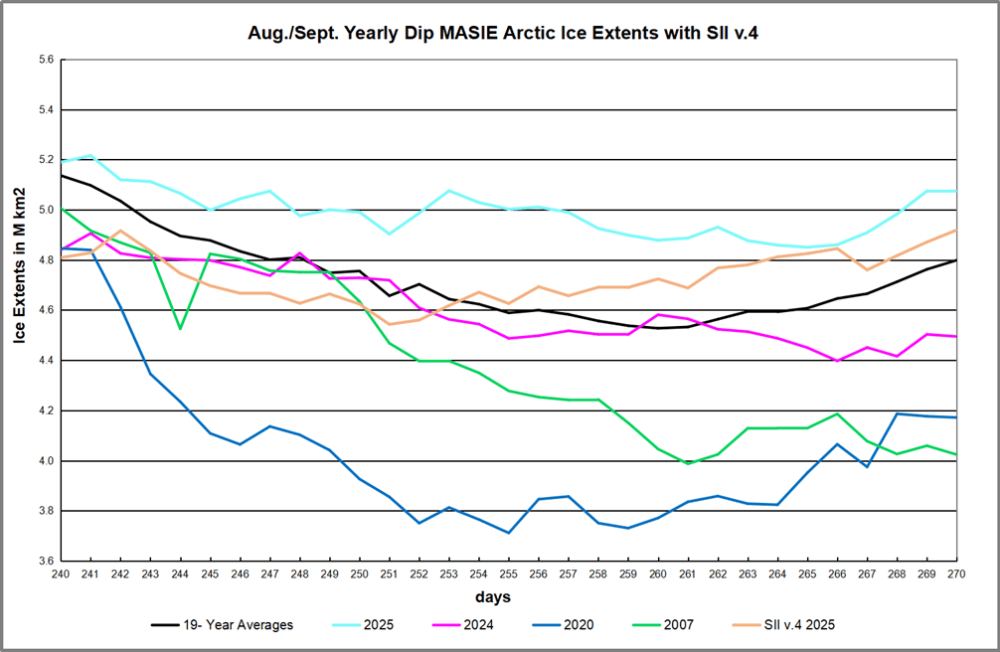
The UAH dataset includes temperature results for air above the oceans, and thus should be most comparable to the SSTs. There is the additional feature that ocean air temps avoid Urban Heat Islands (UHI).  The graph below shows monthly anomalies for ocean air temps since January 2015.

In 2021-22, SH and NH showed spikes up and down while the Tropics cooled dramatically, with some ups and downs, but hitting a new low in January 2023. At that point all regions were more or less in negative territory.

After sharp cooling everywhere in January 2023, there was a remarkable spiking of Tropical ocean temps from -0.5C up to + 1.2C in January 2024.  The rise was matched by other regions in 2024, such that the Global anomaly peaked at 0.86C in April. Since then all regions have cooled down sharply to a low of 0.27C in January.  In February 2025, SH rose from 0.1C to 0.4C pulling the Global ocean air anomaly up to 0.47C, where it stayed in March and April. In May drops in NH and Tropics pulled the air temps over oceans down despite an uptick in SH. At 0.43C, ocean air temps were similar to May 2020, albeit with higher SH anomalies. Now in August Global ocean temps are little changed since SH rose, offsetting NH cooling and Tropics plummenting down to 0.16C from its peak of 1.24C March 2024.

Land Air Temperatures Tracking in Seesaw Pattern

We sometimes overlook that in climate temperature records, while the oceans are measured directly with SSTs, land temps are measured only indirectly.  The land temperature records at surface stations sample air temps at 2 meters above ground.  UAH gives tlt anomalies for air over land separately from ocean air temps.  The graph updated for August is below.

Here we have fresh evidence of the greater volatility of the Land temperatures, along with extraordinary departures by SH land.  The seesaw pattern in Land temps is similar to ocean temps 2021-22, except that SH is the outlier, hitting bottom in January 2023. Then exceptionally SH goes from -0.6C up to 1.4C in September 2023 and 1.8C in  August 2024, with a large drop in between.  In November, SH and the Tropics pulled the Global Land anomaly further down despite a bump in NH land temps. February showed a sharp drop in NH land air temps from 1.07C down to 0.56C, pulling the Global land anomaly downward from 0.9C to 0.6C. In March that drop reversed with both NH and Global land back to January values, holding there in April.  In May sharp drops in NH and Tropics land air temps pulled the Global land air temps back down close to February value. In August Tropics land air dropped sharply, down from 0.58C to 0.26C, and NH land also cooled by 0.1C, offset by SH rising, resulting in no change of Global land air temps.
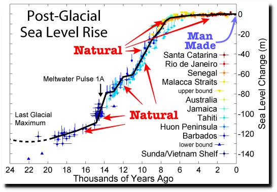
The Bigger Picture UAH Global Since 1980

The chart shows monthly Global Land and Ocean anomalies starting 01/1980 to present.  The average monthly anomaly is -0.0, 2for this period of more than four decades.  The graph shows the 1998 El Nino after which the mean resumed, and again after the smaller 2010 event. The 2016 El Nino matched 1998 peak and in addition NH after effects lasted longer, followed by the NH warming 2019-20.   An upward bump in 2021 was reversed with temps having returned close to the mean as of 2/2022.  March and April brought warmer Global temps, later reversed

With the sharp drops in Nov., Dec. and January 2023 temps, there was no increase over 1980. Then in 2023 the buildup to the October/November peak exceeded the sharp April peak of the El Nino 1998 event. It also surpassed the February peak in 2016. In 2024 March and April took the Global anomaly to a new peak of 0.94C.  The cool down started with May dropping to 0.9C, and in June a further decline to 0.8C.  October went down to 0.7C,  November and December dropped to 0.6C. Now in August Global Land and Ocean is down to 0.39C

The graph reminds of another chart showing the abrupt ejection of humid air from Hunga Tonga eruption.

TLTs include mixing above the oceans and probably some influence from nearby more volatile land temps.  Clearly NH and Global land temps have been dropping in a seesaw pattern, nearly 1C lower than the 2016 peak.  Since the ocean has 1000 times the heat capacity as the atmosphere, that cooling is a significant driving force.  TLT measures started the recent cooling later than SSTs from HadSST4, but are now showing the same pattern. Despite the three El Ninos, their warming had not persisted prior to 2023, and without them it would probably have cooled since 1995.  Of course, the future has not yet been written.