Precipitation Misunderstandings


A previous post on Temperature Misunderstandings addressed mistaken notions about the meaning of temperature measurements and records. This post looks at rainfall, the other primary determinant of climates. For this topic California provides the means for everyone to see how misconceptions arise, and how to see precipitation statistics in context.

Lessons learned from the end of California’s “permanent drought”

A report by Larry Kummer documents how extensively California’s recent shortage of water was proclaimed as a “permanent drought”. And it goes on to document how El Nino conditions have ended the water shortage.

Status of the California drought

“During the past week, a series of storms bringing widespread rain and snow showers impacted the states along the Pacific Coast and northern Rockies. In California, the cumulative effect of several months of abundant precipitation has significantly improved drought conditions across the state.”
— US Drought monitor – California, February 9.

Precipitation over California in the water year so far (October 1 to January 31) is 178% of average for this date. The snowpack is 179% of average, as of Feb 8. Our reservoirs are at 125% of average capacity. See the bottom line summary as of February 7, from the US Drought monitor for California.

The improvement has been tremendous. The area with exceptional drought conditions have gone year over year from 38% of California to 0%, extreme drought from 23% to 1%, severe drought from 20% to 10% — while dry and moderate drought went from 18% to 48%, and no drought from <1% to 41%. See the map below. And the rain continues to fall.

In addition there is the saga of Oroville dam threatened by its reservoir overfilling.

Confusing Weather and Climate

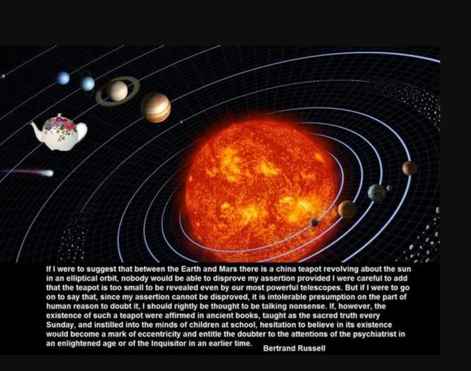
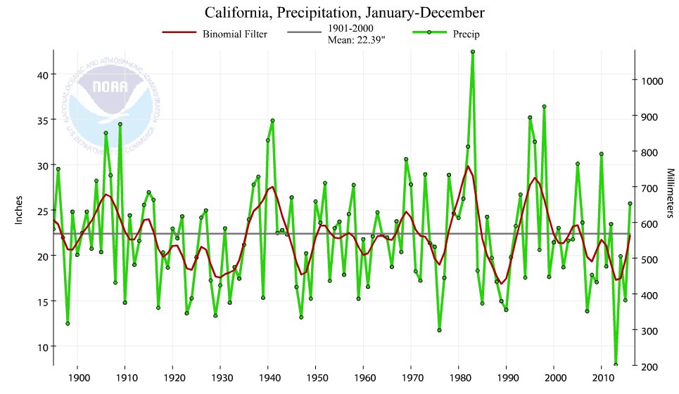
As with temperature, rainy weather is not climate. Neither is fair, sunny weather permanent. Precipitation is variable in any particular climate, with the seasons and on decadal and mult-decadal bases. For a context on precipitation patterns around the world see Here Comes the Rain Again.

It is a mistake to call a temporary lack of rain a drought, or worse a permanent drought, and equally a mistake to call a return of rainfall the end of a drought. California’s history as a desert environment does not change just because politicians and the public have short memories.

H/T to Eric Simpson for reminding us of that history:

There is also this perceptive comment by tomholsinger

I wouldn’t be so quick about the drought ending. Droughts are ALWAYS multi-season events. I was very impressed by the references below, which made the point that the 20th Century average of ~200 million acre feet of precipitation in California (rain and snow combined) is way more than the average of ~140 million acre feet over the last 2000 years.

Drying of the West, National Geographic

The West without Water: What Past Floods, Droughts, and Other Climatic Clues Tell Us about Tomorrow, Ingram, B. Lynn, and Malamud-Roam, Frances, 2013, University of California Press

Tom goes on to quote himself from a Modesto Bee op-ed almost two years ago.

Global warming has nothing to do with this – history is bad enough. A long-standing pre-industrial regional climate fluctuation seems underway, returning us from the wettest century in the past 1000 years to at least the historic average of much less (~70%) rain and snow. Many paleoclimatologists believe we are entering a still worse mega-drought .

An extreme drought by historic standards means a drop to 35-40% of the 20th Century average for 10-20 years. California has experienced two centuries-long such extreme mega-droughts in the past 2000 years.

Our average 20th Century precipitation (rain and snow combined) produced about 200 million acre feet of water annually over the whole state. 118 million acre feet went to nature in 2000, and 82 million was allocated by humans – the first 39 million for federal mandates, 9 million was used by people and industry, and the last 34 million for irrigation. A drop to the historic average of ~140 million acre feet over the past 2000 years means extinction for California agriculture – it would bear almost all the burden of the decrease even if the federal water is released. An extreme drought means a drop to about 75 million acre feet, and we might be starting 1-2 centuries of that.

This is happening to the entire Southwest . ~20 million acre feet of the Southwest’s precipitation annually entered the Colorado River in the 20th Century, of which ~12 million is currently withdrawn by Americans. Colorado River flow too has averaged much less over the past 2000 years (12-14 million acre fee annually), and it drops to 7-8 million in droughts which sometimes last centuries.

A drop to only the historic average precipitation over the past 2000 years means catastrophe for the Southwest. 2/3 of the very wet 20th Century average is normal for the entire area. We can expect ALL of California’s allotment of Colorado River to be diverted to urban areas in Arizona and Nevada in the decades of drought the region seems to be entering.

Summary

As with temperatures, changes in precipitation are misinterpreted when taken out of historical context. This is usually done to hype a sociopolitical agenda by distracting people from the baseline realities to which we can only adapt, not prevent.

The rainfall measures above show that California enjoyed an unusually wet century and it would have been prudent to take advantage of it by storing water resources. As the fable tells us, grasshoppers live for today, ants prepare for tomorrow.

AMO: Atlantic Climate Pulse

I was inspired by David Dilley’s weather forecasting based upon Atlantic water pulsing into the Arctic Ocean (see post: Global Weather Oscillations). So I went looking for that signal in the AMO dataset, our best long-term measure of sea surface temperature variations in the North Atlantic.

ATLANTIC MULTI-DECADAL OSCILLATION (AMO)

For this purpose, I downloaded the AMO Index from Kaplan SST v.2, the unaltered and untrended dataset. By definition, the data are monthly average SSTs interpolated to a 5×5 grid over the North Atlantic basically 0 to 70N.

For an overview the graph below presents a comparison between Annual, March and September averages from 1856 to 2016 inclusive.

amo-march-sept

We see about 4°C difference between the cold month of March, and warm September. The overall trend is slightly positive at 0.27°C per century, about 10% higher in September and 10% lower in March. It is also clear that monthly patterns resemble closely the annual pattern, so it is reasonable to look more closely into Annual variability.

The details of the Annual fluctuations in AMO reveal the pulse pattern suggested by Dilley.

amo-pulses-2

We note firstly the classic pattern of temperature cycles seen in all datasets featuring quality-controlled unadjusted data. The low in 1913, high in 1944, low in 1975, and high in 1998. Also evident are the matching El Nino years 1998, 2009 and 2016, indicating that what happens in the Pacific does not stay in the Pacific.

Most interesting are the periodic peaking of AMO in the 8 to 10 year time frame. The arrows indicate the peaks, which as Dilley describes produce a greater influx of warm Atlantic water under the Arctic ice. And as we know from historical records and naval ice charts, Arctic ice extents were indeed low in the 1930s, high in the 1970s, low in the 1990s and on a plateau presently.

Conclusion

I am intrigued but do not yet subscribe to the Lunarsolar explanation for these pulses, but the AMO index does provide impressive indication of the North Atlantic role as a climate pacemaker. Oceans make up 71% of the planet surface, so SSTs directly drive global mean temperatures (GMT). But beyond the math, Atlantic pulses set up oscillations in the Arctic that impact the world.

In the background is a large scale actor, the Atlantic Meridional Overturning Circulation (AMOC) which is the Atlantic part of the global “conveyor belt” moving warm water from the equatorial oceans to the poles and back again.  For more on this deep circulation pattern see Climate Pacemaker: The AMOC

Fact: Future Will be Flatter Not Hotter

Another powerful post by Clive Best on how earth’s surface temperatures change by means of changing meridional heat transfers. Meridional Warming.

The key point for me was seeing how the best geological knowledge proves beyond the shadow of a doubt how the earth’s climate profile shifts over time, as presented in the diagram above.  It comes from esteemed paleoclimatologist Christopher Scotese.  His compete evidence and analysis can be reviewed in his article Some thoughts on Global Climate Change: The Transition from Icehouse to Hothouse (here).

In that essay Scotese shows where we are presently in this cycle between icehouse and hothouse.

As of 2015 earth is showing a GMT of 14.4C, compared to pre-industrial GMT of 13.8C.  According to the best geological evidence from millions of years of earth’s history, that puts us in the category “Severe Icehouse.”  So, thankfully we are warming up, albeit very slowly.

Moreover, and this is Clive Best’s point, progress toward a warming world means flattening the profile at the higher latitudes, especially the Arctic.  Equatorial locations remain at 23C throughout the millennia, while the gradient decreases in a warmer world.

The previous post explained what is wrong with averaging temperature anomalies.  See Temperature Misunderstandings

Conclusion:

We have many, many centuries to go before the earth can warm up to the “Greenhouse” profile, let alone get to “Hothouse.”  Regional and local climates at higher latitudes will see slightly warming temperatures and smaller differences from equatorial climates.  These are facts based on solid geological evidence, not opinions or estimates from computer models.

It is still a very cold world, but we are moving in the right direction.  Stay the course.

Meanwhile, keep firing away Clive.

damaged-ship3


Temperature Misunderstandings

Clive Best provides this animation of recent monthly temperature anomalies which demonstrates how most variability in anomalies occur over northern continents.

Beyond the issues with the measurements and the questionable adjustments, there is a more fundamental misconception about air temperatures in relation to “climate change.” Clive Best does a fine job explaining why Global Mean Temperature anomalies do not mean what people think. Below is my synopsis of his recent essay entitled Do Global Temperatures make sense? (link)

Background: Earth’s Heat Imbalance

ERBE measurements of radiative imbalance.

The earth’s temperature at any location is never in equilibrium. It changes daily, seasonally and annually. Incoming solar radiation varies enormously especially near the poles which receive more energy per day in summer than the equator.

The earth cools primarily by moving heat from hot tropical regions towards high latitudes where net IR radiation loss cools the planet, thus maintaining a certain temperature profile.

Key Point: Heat Distribution Changes, not Global Temperatures

Rising CO2 levels modify that radiation imbalance profile slightly. Surface temperatures in the tropics are not really warming at all. Any excess heat induces more clouds and more convection while surface temperatures remain constant. What really happens is that the meridional radiation profile changes. Slightly more heat is transported polewards so that hot places are shifting more heat to cold places which are doing the warming. If CO2 levels stop rising then a new temperature and radiation profile would rather quickly be reached. This is then called ‘climate change’ but any such changes are concentrated in colder regions of the world. The global ‘temperature’ itself is not changing, but instead the global distribution of temperature is changing.

Key Point: More Atmospheric Heat means Warming in the Coldest Places

Temperatures at the poles during 6 months of darkness would fall well below -150C if there was no atmosphere, similar to the moon. Instead heat is constantly being transported from lower latitudes by the atmosphere and ocean and so that temperatures never fall much below -43C. If more heat is transported northwards than previously, then minimum temperatures must rise, and this is what we observe in individual measurements.

Key Point: GMT Anomalies Are Dominated by the Highest Latitudes

The main problem with all the existing observational datasets is that they don’t actually measure the global temperature at all. Instead they measure the global average temperature ‘anomaly’. . .The use of anomalies introduces a new bias because they are now dominated by the larger ‘anomalies’ occurring at cold places in high latitudes. The reason for this is obvious, because all extreme seasonal variations in temperature occur in northern continents, with the exception of Antarctica. Increases in anomalies are mainly due to an increase in the minimum winter temperatures, especially near the arctic circle. 

To take an extreme example here is the monthly temperature data and calculated anomalies for Verkoyhansk in Siberia. Annual temperatures vary from -50C in winter to +20C in summer. That is a seasonal range of 70C each year, and a year to year anomaly variation of ~8C is normal. The only global warming effect evident is a slight increase in the minimum winter temperatures since 1900. That is not due to any localised enhanced greenhouse effect but rather to an enhanced meridional heat transport. Temperatures in equatorial regions meanwhile have only ~4C seasonal variations, and show essentially no warming trend.

Long term changes in temperature anomalies occur mainly in northern continents in winter months. This is not because the earth as a whole is warming up but rather that meridional heat transport from the equator to the poles has increased and the largest effect on ‘anomalies occurs in winter. The average absolute temperature of the earth’s surface is unknown. Basing the evidence for climate change on the 150 year trend in global averaged temperature anomalies still biases the result towards higher latitudes where most of the stations are located.

Summary

When heat is released into the atmosphere from the oceans, it is transported toward the poles to dissipate into space. Places in higher latitudes are warmed, not by radiative effects of greenhouse gases in those locales, but by the incursion of warmer air from the equator.

What happens if more CO2 is added into the atmosphere? No one knows, but there are many opinions, a popular one being that more heat is retained in the atmosphere. But in that case, that additional heat will be shed by the planet in exactly the same manner: transport to the poles with slightly less extremely cold air at the higher latitudes.

Why in the world would we pay anything to prevent a little bit of warming in the world’s coldest places?

Clive Best takes the analysis further and relates to work by Christopher Scotese in a later post Fact: Future Climate Will Be Flatter, not Hotter

Footnote: Scott Pruitt provides a concise synopsis of the issues in measuring global surface temperatures.  From his responses to Senators’ questions during confirmation hearings:

Senator Merkley:

Are you aware that each of the past three decades has been warmer than the one before, and warmer than all the previous decades since record keeping began in the 1880s? This trend is based on actual temperature measurements. Do you believe that there is uncertainty in this warming trend that has been directly measured? If so, please explain.

Nominee Pruitt:

I am aware of a diverse range of conclusions regarding global temperatures, including that over the past two decades satellite data indicates there has been a leveling off of warming, which some scientists refer to as the “hiatus.”
I am also aware that the discrepancy between land-based temperature stations and satellite temperature stations can be attributed to expansive urbanization within in our country where artificial substances such as asphalt can interfere with the accuracy of land-based temperature stations and that the agencies charged with keeping the data do not accurately account for this type of interference.
I am also aware that ‘warmest year ever’ claims from NASA and NOAA are based on minimal temperature differences that fall within the margin of error.
Finally, I am aware that temperatures have been changing for millions of years that predate the relatively short modern record keeping efforts that began in 1880.

More Q&A is at Running the Climate Gauntlet

More explanation at The Climate Water Wheel

The Climate Change Teapot

The confirmation hearings with questions from global warming zealots reminded me of Bertrand Russell’s teapot analogy.

The notion of global warming/climate change resembles closely that mythical teapot.  People like Lewandowsky and Oreskes psychoanalyze unbelievers.  And public hearings are conducted to uncover unseemly heresy inside political appointees.  At least when religion is recognized as such, and not confused with science, modern societies understand it is a matter of opinion and freedom of thought and expression is accepted.


Clamatology

clamSome reporters are showing an interest in a lesser known proxy for climate change: giant clams. Of course, some scientists claim clams prove unprecedented global warming this century. Unsurprising since their funding (clams) depends on sounding the alarms.

For some insight into the connection between clams and climate, here is a paper Giant clam recorders of ENSO variability (here).

Giant clam stable isotope profiles from Papua New Guinea faithfully record all the major El Niño events between 1986 and 2003, thus illustrating the usefulness of this archive to reconstruct past ENSO variability. Elliott et al.

In northern Papua New Guinea precipitation and temperatures are coupled on seasonal and interannual timescales. El Niño periods are associated with lower than average SST and drier conditions, whereas La Niña periods are associated with higher than average SST and wetter conditions. The associated changes in sea water δ18O and SST will thus have cumulative effects on shell δ18O, which will become more positive during El Niño and more negative during La Niña phases.

clam-fig2

Figure 2: Comparison of T. gigas δ18O profile with ENSO index, local temperature and rainfall data. A) NINO3.4 index, (B) 3pt smoothed monthly rainfall anomaly (mm day-1, NASA/GPCPV2) for 146.25°E, 6.25°S, (C) T. gigas δ18O record, (D) Porites δ18O profiles and (E) 3pt smoothed monthly SST anomaly (from IGOSS) for the same grid box as the rainfall data. Y-axes of the δ18O are inverted. The shaded bands indicate El Niño events.

The comparison of the ENSO index with the T. gigas and Porites δ18O records shows that each El Niño event is recorded in the shell and coral profile by isotopic shifts of around 1.0 to 1.2‰ toward more positive values (Fig. 2) reflecting the combined influence of lower temperatures and decreased rainfall. During the El Niño phase of the Southern Oscillation, the region experiences relative drought and slightly reduced SSTs (~-0.2 to -0.5°C anomaly, see Fig. 2). These factors combine to drive skeletal δ18O to heavy values, with SST explaining about 30-50% of the skeletal δ18O range.

Take away message

We show that shells of T. gigas can be used to produce multi-decadal climatic records, hence providing a valuable resource for investigating changes to the frequency and strength of ENSO events in the past. The excellent reproducibility of clam and coral δ18O profiles illustrates the strength of using these archives to reconstruct large-scale hydrographic changes.

Some points worth noting: Clamshell variability is influenced by precipitation as well as water temperature. And water temperatures do not simply correlate to air temperatures. Finally, it is the water heating the air, not the other way around.

The data is good, but the interpretation can be biased by warmist beliefs.

Three Wise Men Talking Climate

Everyone is entitled to their opinion on climate change, although renowned theoretical physicists may be especially persuasive. This post compares quotes from 3 of the most distinguished: Stephen Hawking (much in the news lately since Trump’s election), Freeman Dyson and Richard Feynman. Hawking is an alarmist, Dyson a skeptic and Feynman concerned about scientific integrity.

Stephen Hawking is a phenomenal human being, original thinker on grand design and genuinely concerned about humanity and our planetary home. His own battle with frailty gives weight to his opinions and observations. Thus when he meets with the Pope or Al Gore and warns about future global warming, many people will take his words seriously.

Comments on Climate Change by Stephen Hawking

On May 31, 2016 he said: “A more immediate danger is runaway climate change,” Hawking said. “A rise in ocean temperature would melt the ice-caps, and cause a release of large amounts of carbon dioxide from the ocean floor. Both effects could make our climate like that of Venus, with a temperature of 250 degrees.”

“Six years ago I was warning about pollution and overcrowding, they have gotten worse since then,” Hawking said. “The population has grown by half a billion since our last meeting with no end in sight. At this rate, it will be 11 billion by 2100. Air pollution has increased by 8 percent over the past five years.”

Elsewhere he has said, “I don’t think we will survive another 1,000 years without escaping beyond our fragile planet,” going on express concerns about consuming earth’s natural resources, nuclear war, climate change, genetically-engineered viruses and the rise of artificial intelligence spelling planetary doom.

Those are his opinions, not shared by other equally distinguished theoretical physicists, two examples being Freeman Dyson and Richard Feynman.

Freeman Dyson is best known for his contribution to Quantum Electrodynamics. Quantum Electrodynamics is the field where scientists study the interaction of electromagnetic radiation with electrically charged matter within the framework of relativity and quantum mechanics. Dyson wrote two books on the subject of Quantum Electrodynamics. His books influence many branches of modern day theoretical physics.

In his quest to expand our world of knowledge, properly control nuclear power, and discover more information on quantum electrodynamics, Freeman Dyson has written a large collection of books that explains how he believes that the world should grow more efficiently.

Comments on Climate Change by Freeman Dyson

I was in the business of studying climate change at least 30 years ago before it became fashionable. The idea that global warming is the most important problem facing the world is total nonsense and is doing a lot of harm. It distracts people’s attention from much more serious problems.

When I listen to the public debates about climate change, I am impressed by the enormous gaps in our knowledge, the sparseness of our observations and the superficiality of our theories.

We simply don’t know yet what’s going to happen to the carbon in the atmosphere.

We do not know how much of the environmental change is due to human activities and how much [is due] to long-term natural processes over which we have no control.

Computer models of the climate….[are] a very dubious business if you don’t have good inputs.

To any unprejudiced person reading this account, the facts should be obvious: that the non-climatic effects of carbon dioxide as a sustainer of wildlife and crop plants are enormously beneficial, that the possibly harmful climatic effects of carbon dioxide have been greatly exaggerated, and that the benefits clearly outweigh the possible damage.

The people who are supposed to be experts and who claim to understand the science are precisely the people who are blind to the evidence. Those of my scientific colleagues who believe the prevailing dogma about carbon dioxide will not find Goklany’s evidence convincing. . .That is to me the central mystery of climate science. It is not a scientific mystery but a human mystery. How does it happen that a whole generation of scientific experts is blind to obvious facts?

Richard Feynman revolutionized the field of quantum mechanics through conceiving the Feynman path integral, and by inventing Feynman diagrams for doing relativistic quantum mechanical calculations. Further he won the Nobel prize for his theory of quantum electrodynamics, and finally in particle physics he proposed the parton model to analyze high-energy hadron collisions.  He died in 1988 before global warming obsession was popularized, and so his comments apply mainly to how scientific theories should be treated with integrity.

Comments on Scientific Integrity by Richard Feynman

How Science Works: “In general, we look for a new law by the following process. First, we guess it (audience laughter), no, don’t laugh, that’s really true. Then we compute the consequences of the guess, to see what, if this is right, if this law we guess is right, to see what it would imply and then we compare the computation results to nature, or we say compare to experiment or experience, compare it directly with observations to see if it works.  If it disagrees with experiment, it’s wrong. In that simple statement is the key to science. It doesn’t make any difference how beautiful your guess is, it doesn’t matter how smart you are, who made the guess, or what his name is… If it disagrees with experiment, it’s wrong. That’s all there is to it.”

It’s a kind of scientific integrity, a principle of scientific thought that corresponds to a kind of utter honesty–a kind of leaning over backwards. For example, if you’re doing an experiment, you should report everything that you think might make it invalid–not only what you think is right about it: other causes that could possibly explain your results; and things you thought of that you’ve eliminated by some other experiment, and how they worked–to make sure the other fellow can tell they have been eliminated.

Details that could throw doubt on your interpretation must be given, if you know them. You must do the best you can–if you know anything at all wrong, or possibly wrong–to explain it. If you make a theory, for example, and advertise it, or put it out, then you must also put down all the facts that disagree with it, as well as those that agree with it. There is also a more subtle problem. When you have put a lot of ideas together to make an elaborate theory, you want to make sure, when explaining what it fits, that those things it fits are not just the things that gave you the idea for the theory; but that the finished theory makes something else come out right, in addition.

Summary

Hawking has gone to the dark side, foreseeing disaster from numerous modern developments, and includes climate change without challenging the precepts with his considerable critical intelligence. Dyson has analyzed radiative activity in quantum electrodynamics and sees clearly that effects from humanity’s minuscule addition to the trace gas CO2 does far more good for the biosphere than it does harm. Feynman encourages us not to accept answers claimed to be unquestionable.

This post was inspired by Lubos Motl, who blogged similarly on another issue (here), and Ivar Giaever who has long spoken out against alarmist claims. Two more outstanding physicists who have actually examined global warming claims and found them wanting.

On Warming Holes (Global Warming Gaps)


Animation showing the 25-year and 40-year trends in surface air temperature in the Cowtan and Way v2.0 dataset, with plots to the right showing the fraction of the earth surface in a cooling trend (the blue areas in maps).

Ed Hawkins at his blog provides above the display of variability of warming and cooling across the globe. The post is entitled Regional Temperatures This Century (here).

We found that some regions experience periods of cooling at this timeframe even when global temperature is increasing rapidly. Cooling periods of 25 years duration occurred in 13 to 74 % of the earth surface through the observed record, and cooling periods of 40 years occurred in 6 to 71% of the earth surface, including in the most recent decades. Cooling periods are more prevalent where the long-term trend is low such as in the Southern Ocean, and/or where decadal variability is high such as Pacific Ocean regions influenced by the Inter-Decadal Pacific Oscillation (IPO). However, there are cases where low trend or high variability due to the IPO (or Atlantic Multi-decadal Oscillation) are not the only factors, and there may be a role for forcings and other regional effects. These cases include the well-known ‘warming hole’ in the south east US through the last half of the 20th Century (noting this ‘hole’ has an important seasonal aspect to it) and the recent cooling in northern Australia linked to increasing cloud and rainfall.

He refers to the cooling regions as “warming holes”. Since there are periods where cooling dominates globally, we could also refer to exceptional regions as “warm spots.” This shows dynamically how regional climate trends differ over time. For example, over the last century in the continental US, about a third of land stations showed cooling trends contrary to the slightly warming average overall.

Cautionary note regarding the Cowtan and Way 2.0 Dataset

This dataset is controversial in its use of “krieging” to spread temperature readings from a handful of land stations across the full extent of the Arctic (and Antarctic) including surfaces of ocean, ice and mixtures of the two. As the charts show, this results in extra warming in the Arctic, double the trend shown by UAH (satellite) dataset.

Another example of the inconsistency of “global warming” is provided by NOAA’s presentation of continental temperatures. (here) The table below is for October 2016, and shows not only variability, but also how land temperatures are falling following El Nino’s disappearance.

CONTINENT ANOMALY (1910-2000) TREND (1910-2016) RANK
(OUT OF 107 YEARS)
RECORDS
°C °F °C °F YEAR(S) °C °F
North America +1.33 +2.39 +0.05 +0.09 Warmest 7ᵗʰ 1963 +2.16 +3.89
Coolest 101ˢᵗ 1919 -1.94 -3.49
South America +0.85 +1.53 +0.17 +0.30 Warmest 15ᵗʰ 2014 +1.60 +2.88
Coolest 92ⁿᵈ 1922 -1.04 -1.87
Ties: 1994
Europe +0.40 +0.72 +0.11 +0.20 Warmest 41ˢᵗ 2006, 2001 +1.96 +3.53
Coolest 67ᵗʰ 1912 -1.99 -3.58
Africa +1.35 +2.43 +0.09 +0.16 Warmest 2ⁿᵈ 2015 +1.59 +2.86
Coolest 106ᵗʰ 1910 -0.65 -1.17
Asia -0.15 -0.27 +0.10 +0.18 Warmest 69ᵗʰ 2011 +1.76 +3.17
Coolest 39ᵗʰ 1912 -2.22 -4.00
Oceania +0.21 +0.38 +0.13 +0.23 Warmest 44ᵗʰ 2015 +2.71 +4.88
Coolest 64ᵗʰ 1910 -1.15 -2.07


Putting Climate Models in Their Place

A previous post Chameleon Climate Models described the general issue of whether a model belongs on the bookshelf (theoretically useful) or whether it passes real world filters of relevance, thus qualifying as useful for policy considerations.

Following an interesting discussion on her blog, Dr. Judith Curry has written an important essay on the usefulness and limitations of climate models.

The paper was developed to respond to a request from a group of lawyers wondering how to regard claims based upon climate model outputs. The document is entitled Climate Models (here) and is a great informative read for anyone. Some excerpts that struck me:

Climate model development has followed a pathway mostly driven by scientific curiosity and computational limitations. GCMs were originally designed as a tool to help understand how the climate system works. GCMs are used by researchers to represent aspects of climate that are extremely difficult to observe, experiment with theories in a new way by enabling hitherto infeasible calculations, understand a complex system of equations that would otherwise be impenetrable, and explore the climate system to identify unexpected outcomes. As such, GCMs are an important element of climate research.

Climate models are useful tools for conducting scientific research to understand the climate system. However, the above points support the conclusion that current GCM climate models are not fit for the purpose of attributing the causes of 20th century warming or for predicting global or regional climate change on timescales of decades to centuries, with any high level of confidence. By extension, GCMs are not fit for the purpose of justifying political policies to fundamentally alter world social, economic and energy systems. It is this application of climate model results that fuels the vociferousness of the debate surrounding climate models.

Evolution of state-of-the-art Climate Models from the mid 70s to the mid 00s. From IPCC (2007)

Evolution of state-of-the-art Climate Models from the mid 70s to the mid 00s. From IPCC (2007)

The actual equations used in the GCM computer codes are only approximations of the physical processes that occur in the climate system. While some of these approximations are highly accurate, others are unavoidably crude. This is because the real processes they represent are either poorly understood or too complex to include in the model given the constraints of the computer system. Of the processes that are most important for climate change, parameterizations related to clouds and precipitation remain the most challenging, and are the greatest source of disagreement among different GCMs.

There are literally thousands of different choices made in the construction of a climate model (e.g. resolution, complexity of the submodels, parameterizations). Each different set of choices produces a different model having different sensitivities. Further, different modeling groups have different focal interests, e.g. long paleoclimate simulations, details of ocean circulations, nuances of the interactions between aerosol particles and clouds, the carbon cycle. These different interests focus their limited computational resources on a particular aspect of simulating the climate system, at the expense of others.


Overview of the structure of a state-of-the-art climate model. See Climate Models Explained by R.G. Brown

Human-caused warming depends not only on how much CO2 is added to the atmosphere, but also on how ‘sensitive’ the climate is to the increased CO2. Climate sensitivity is defined as the global surface warming that occurs when the concentration of carbon dioxide in the atmosphere doubles. If climate sensitivity is high, then we can expect substantial warming in the coming century as emissions continue to increase. If climate sensitivity is low, then future warming will be substantially lower.

In GCMs, the equilibrium climate sensitivity is an ‘emergent property’ that is not directly calibrated or tuned. While there has been some narrowing of the range of modeled climate sensitivities over time, models still can be made to yield a wide range of sensitivities by altering model parameterizations. Model versions can be rejected or not, subject to the modelers’ own preconceptions, expectations and biases of the outcome of equilibrium climate sensitivity calculation.

Further, the discrepancy between observational and climate model-based estimates of climate sensitivity is substantial and of significant importance to policymakers. Equilibrium climate sensitivity, and the level of uncertainty in its value, is a key input into the economic models that drive cost-benefit analyses and estimates of the social cost of carbon.

Variations in climate can be caused by external forcing, such as solar variations, volcanic eruptions or changes in atmospheric composition such as an increase in CO2. Climate can also change owing to internal processes within the climate system (internal variability). The bestknown example of internal climate variability is El Nino/La Nina. Modes of decadal to centennial to millennial internal variability arise from the slow circulations in the oceans. As such, the ocean serves as a ‘fly wheel’ on the climate system, storing and releasing heat on long timescales and acting to stabilize the climate. As a result of the time lags and storage of heat in the ocean, the climate system is never in equilibrium.

The combination of uncertainty in the transient climate response (sensitivity) and the uncertainties in the magnitude and phasing of the major modes in natural internal variability preclude an unambiguous separation of externally forced climate variations from natural internal climate variability. If the climate sensitivity is on the low end of the range of estimates, and natural internal variability is on the strong side of the distribution of climate models, different conclusions are drawn about the relative importance of human causes to the 20th century warming.

Figure 5.1. Comparative dynamics of the World Fuel Consumption (WFC) and Global Surface Air Temperature Anomaly (ΔT), 1861-2000. The thin dashed line represents annual ΔT, the bold line—its 13-year smoothing, and the line constructed from rectangles—WFC (in millions of tons of nominal fuel) (Klyashtorin and Lyubushin, 2003). Source: Frolov et al. 2009

Anthropogenic (human-caused) climate change is a theory in which the basic mechanism is well understood, but whose potential magnitude is highly uncertain. What does the preceding analysis imply for IPCC’s ‘extremely likely’ attribution of anthropogenically caused warming since 1950? Climate models infer that all of the warming since 1950 can be attributed to humans. However, there have been large magnitude variations in global/hemispheric climate on timescales of 30 years, which are the same duration as the late 20th century warming. The IPCC does not have convincing explanations for previous 30 year periods in the 20th century, notably the warming 1910-1945 and the grand hiatus 1945-1975. Further, there is a secular warming trend at least since 1800 (and possibly as long as 400 years) that cannot be explained by CO2, and is only partly explained by volcanic eruptions.

Summary

There is growing evidence that climate models are running too hot and that climate sensitivity to CO2 is on the lower end of the range provided by the IPCC. Nevertheless, these lower values of climate sensitivity are not accounted for in IPCC climate model projections of temperature at the end of the 21st century or in estimates of the impact on temperatures of reducing CO2 emissions.

The climate modeling community has been focused on the response of the climate to increased human caused emissions, and the policy community accepts (either explicitly or implicitly) the results of the 21st century GCM simulations as actual predictions. Hence we don’t have a good understanding of the relative climate impacts of the above (natural factors) or their potential impacts on the evolution of the 21st century climate.

Footnote:

There are a series of posts here which apply reality filters to attest climate models.  The first was Temperatures According to Climate Models where both hindcasting and forecasting were seen to be flawed.

Others in the Series are:

Sea Level Rise: Just the Facts

Data vs. Models #1: Arctic Warming

Data vs. Models #2: Droughts and Floods

Data vs. Models #3: Disasters

Data vs. Models #4: Climates Changing

Climate Medicine

Climates Don’t Start Wars, People Do

virtual-reality-1920x1200

Beware getting sucked into any model, climate or otherwise.