Scafetta: Climate Models Have Issues

On June 18, 2025 Nicola Scafetta published Detection, attribution, and modeling of climate change:  key open issues.  Excerpts in italics with my bolds and added images.

Abstract

The Coupled Model Intercomparison Project (CMIP) global climate models (GCMs) assess that nearly 100% of global surface warming observed between 1850–1900 and 2011–2020 is attributable to anthropogenic drivers like greenhouse gas emissions. These models also generate future climate projections based on shared socioeconomic pathways (SSPs), aiding in risk assessment and the development of costly “Net-Zero” climate mitigation strategies.

Figure 1. Anthropgenic and natural contributions. (a) Locked scaling factors, weak Pre Industrial Climate Anomalies (PCA). (b) Free scaling, strong PCA Source: Larminat, P. de (2023)

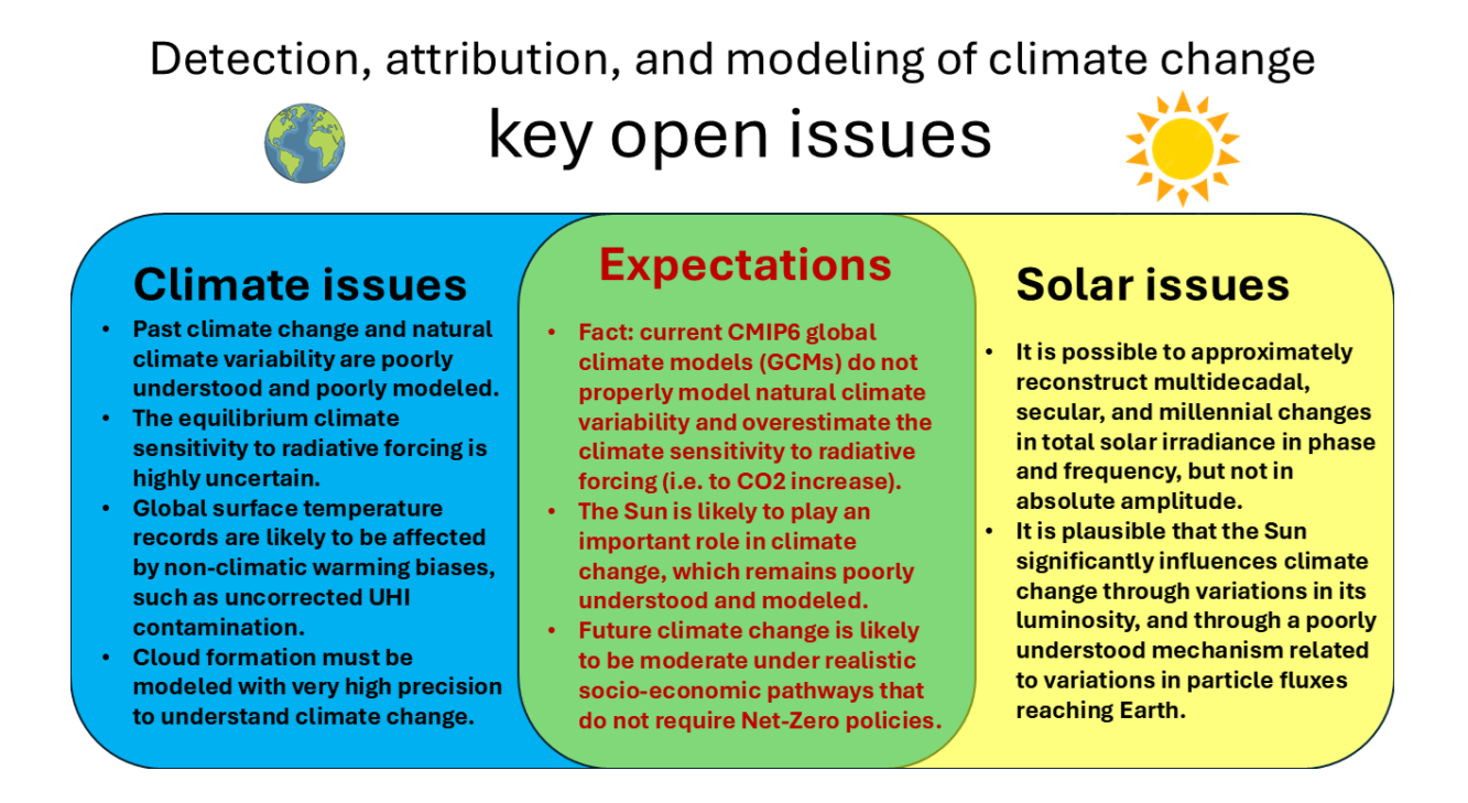
Yet, as this study discusses, the CMIP GCMs face significant scientific challenges in attributing and modeling climate change, particularly in capturing natural climate variability over multiple timescales throughout the Holocene. Other key concerns include the reliability of global surface temperature records, the accuracy of solar irradiance models, and the robustness of climate sensitivity estimates. Global warming estimates may be overstated due to uncorrected non-climatic biases, and the GCMs may significantly underestimate solar and astronomical influences on climate variations.

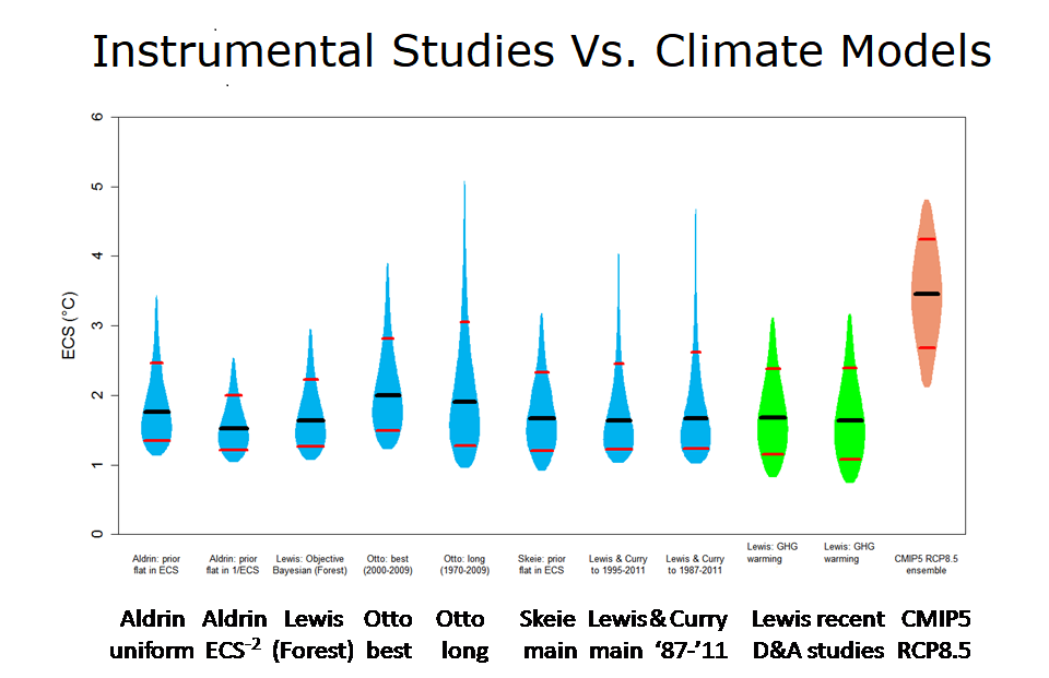
The equilibrium climate sensitivity (ECS) to radiative forcing could be lower than commonly assumed; empirical findings suggest ECS values lower than 3°C and possibly even closer to 1.1 ± 0.4 °C. Empirical models incorporating natural variability suggest that the 21st-century global warming may remain moderate, even under SSP scenarios that do not necessitate Net-Zero emission policies.
These findings raise important questions regarding the necessity and urgency of implementing aggressive climate mitigation strategies. While GCMs remain essential tools for climate research and policymaking, their scientific limitations underscore the need for more refined modeling approaches to ensure accurate future climate assessments. Addressing uncertainties related to climate change detection, natural variability, solar influences, and climate sensitivity to radiative forcing will enhance predictions and better inform sustainable climate strategies.

Discussion

Scientific challenges in climate detection, attribution, and modeling stem from three primary issues:

1. the inherent uncertainty of what measurements really indicate complicates the detection of climate change and its causative factors;
2. the anthropogenic contribution is superimposed to natural climate variability, necessitating comprehensive understanding and accurate modeling of the latter;
3. key physical processes, such as cloud formation and solar contributions to climate dynamics, remain poorly characterized.
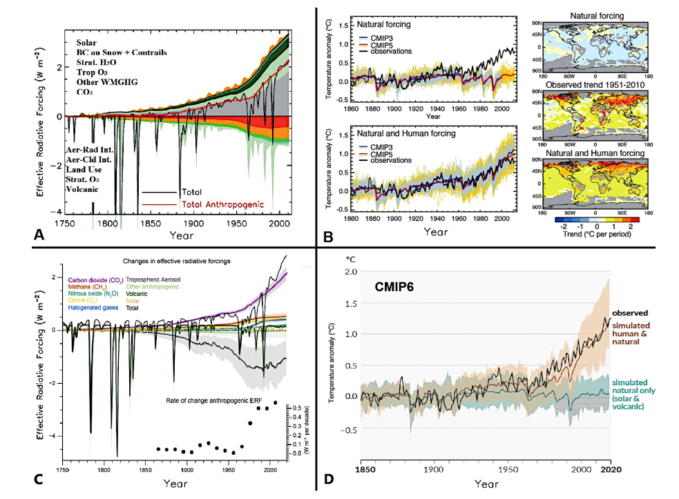
Figure 1:

(A) Compilation of the radiative forcing functions utilized in the CMIP5 GCMs (adapted from IPCC,2013, Figure 8.18).
(B) Variations in observed global surface temperature (black) alongside the CMIP3 and CMIP5 model simulations incorporating only natural forcing and combined natural-anthropogenic forcing (adapted from IPCC, 2013, FAQ 10.1, Figure 1).
(C) Compilation of the radiative forcing functions utilized in the CMIP6 GCMs (adapted from IPCC, 2021, Figure 2.10).
(D) Observed global surface temperature variations (black) alongside the CMIP6 model simulations incorporating only natural forcing and combined naturalanthropogenic forcing (adapted from IPCC, 2021, Figure SPM.1).

Notably, in both (B) and (D), the observational data necessary
to validate the GCM predictions that consider only natural forcings
are not reported because they do not exist.

While all available GCMs indicate that the positive feedbacks surpass the negative ones thus amplifying the effects of radiative forcing, large uncertainties associated with crucial feedback mechanisms — particularly those related to water vapor and cloud formation — remain substantial.

Feedback mechanisms include:

Water Vapor Feedback — A positive feedback governed by the Clausius-Clapeyron law, which links ocean vaporation rates to temperature increases;
Albedo Feedback — A positive feedback arising from changes in surface reflectivity due to ice and snow
cover variations;
Cloud Feedback — Particularly challenging to quantify, as cloud formation, type, and distribution are sensitive to warming; certain clouds cool the surface by reflecting solar radiation, while others trap emitted
heat, making their net contribution highly uncertain;
Lapse Rate Feedback — A negative feedback involving modifications to atmospheric temperature vertical
gradients;
Carbon Cycle Feedback — Activated by warming-induced CO2 release from soils and oceans (per Henry’s law), further increasing atmospheric CO2 concentrations;
Vegetation Feedback — Temperature and precipitation changes alter vegetation cover, which influences
carbon storage and surface albedo.

The CMIP6 GCMs are also employed to simulate future climate scenarios based on hypothetical radiative forcing functions derived from Shared Socioeconomic Pathways (SSPs). The ones mainly adopted in the IPCC AR6 are:
SSP1-2.6 — low greenhouse gas emissions, with robust adaptation and mitigation measures leading to
Net-Zero CO2 emissions between 2050–2075;
• SSP2-4.5 — intermediate emissions, where CO2 levels remain near current levels until 2050 and subsequently decline without achieving Net-Zero by 2100;
• SSP3-7.0 — high emissions, with CO2 concentrations doubling by 2100 under minimal policyintervention;
• SSP5-8.5 — very high emissions, with CO2 levels tripling by 2075 under a worst-case scenario devoid of
mitigation measures.
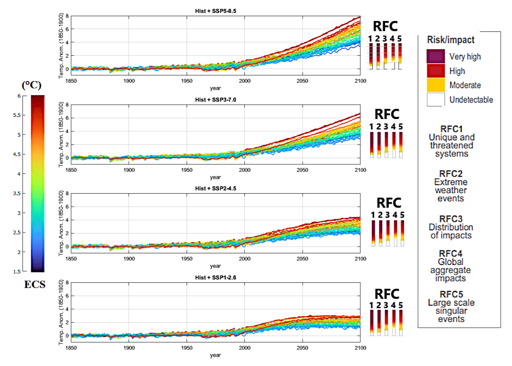
Figure 3: CMIP6 GCM ensemble mean simulations spanning from 1850 to 2100, employing historical effective radiative forcing functions from 1850 to 2014 (see Figure 1C) and the forcing functions based on the SSP scenarios 1-2.6, 2-4.5, 3-7.0, and 5-8.5. Curve colors are scaled according to the equilibrium climate sensitivity (ECS) of the models. The right panels depict the risks and impacts of climate change in relation to various global Reasons for Concern (RFCs) (IPCC, 2023). (Adapted from Scafetta, 2024).

Conclusion

Over the span of approximately three decades, from the publication of the First Assessment Report (FAR, IPCC, 1990) to the Sixth Assessment Report (AR6, IPCC, 2021), the Intergovernmental Panel on Climate Change (IPCC) has significantly advanced  marked up its understanding of the role of anthropogenic emissions in driving global warming.

In the 1990s the IPCC posited that both natural mechanisms and human activities could have contributed roughly equally (∼50% each) to the observed warming of the 20th century. However, since the years 2000s the prevailing scientific opinion has shifted, and the IPCC (AR6, 2021) now asserts that human activities are almost exclusively responsible (∼100%) for the global warming and climate change observed from 1850–1900 to 2011–2020.

The most recent assessment reports IPCC (2021, 2023) underscore this conclusion with striking clarity. As shown in Figure 2, the average contribution of natural factors — solar and volcanic forcing and internal natural variability — to global warming during the aforementioned period is estimated to be approximately 0°C.  Consequently, from the CMIP GCM perspective, concerns about future climate warming due to additional anthropogenic greenhouse gas (GHG) emissions are well-founded. However, this conclusion depends on the reliability of global surface temperature records and the robustness of the physical science underpinning global climate models (GCMs).

The findings outlined above underscore significant uncertainties in climate modeling, climate data, solar records, and solar-climate interactions, leaving unresolved the key question of whether observed warming is primarily driven by anthropogenic factors, natural processes, or their interplay. Empirical methodologies, such as those utilized by Scafetta (2023a, 2024) and Connolly et al. (2023), highlight this ongoing ambiguity.

Concerns are mounting regarding the limitations of the CMIP GCMs employed by the IPCC in its assessment reports from 2007, 2013, and 2021. These models appear unable to accurately replicate natural climate variability across different timescales, highlighting critical unresolved issues in fundamental climate dynamics.Also the magnitude of solar variability across temporal scales requires further investigation, particularly given the strong correlations identified between solar proxy records and climate patterns throughout the Holocene. Schmutz (2021) argued that such strong correlations challenge the validity of the low-variability TSI models, such as those proposed by Matthes et al. (2017), Kopp et al., 2016 and Wu et al. (2018). Since these models serve as solar forcing inputs for the CMIP6 GCMs, their choice needs to be reconsidered.

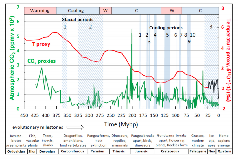
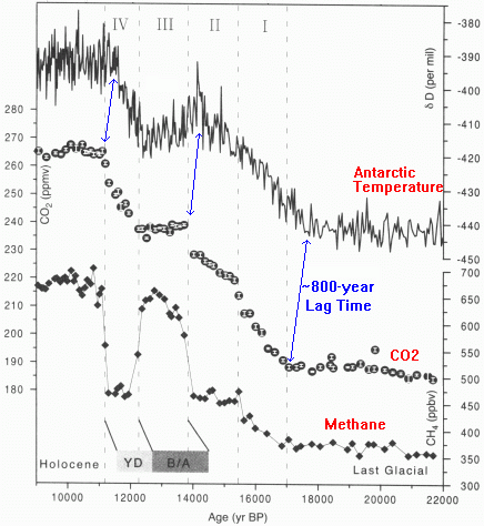
Climate science remains far from settled, yet trillions of dollars continue to be allocated toward policies aimed at mitigating extreme hypothetical warming scenarios based on potentially flawed GCM outputs. Historically, atmospheric CO2 levels have been 10 to 20 times higher than current concentrations during approximately 95% of Earth’s history since complex life emerged 600 million years ago (Davis, 2017). Notably, CO2 concentrations often lag temperature changes across different timescales, suggesting temperature fluctuations may drive CO2 variations rather than vice versa (Shakun et al., 2012; Koutsoyiannis, 2024).
Advancing climate science requires directly confronting uncertainties in detection, attribution, and modeling. Further research on unresolved issues is critical for improving climate risk assessment and developing more effective strategies for addressing future environmental challenges.


2025 Evidence of Nature’s Sunscreen

Greenhouse with adjustable sun screens to control warming.

2025 Updated Report on Global Dimming and Brightening Worldwide and in China 

Martin Wild et al published April 2025 A Perspective on Global Dimming and Brightening Worldwide and in China. Excerpts in italics with my bolds and added images.

Abstract

Worldwide radiation records suggest that the amount of sunlight received at the Earth’s surface (surface solar radiation, SSR) has not been stable over the years, but underwent significant decadal variations, popularly also known as “global dimming and brightening”. These variations have been particularly evident in China, where the SSR substantially declined from the 1960s to the 1990s (dimming), with indications for a trend reversal in the 2000s and a slight recovery (brightening) in recent years. This perspective/review paper will discuss recent updates and remaining challenges regarding our knowledge of the magnitudes, causes, and implications of these variations in SSR worldwide, with a particular emphasis on the developments in China.

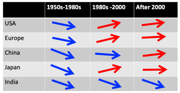
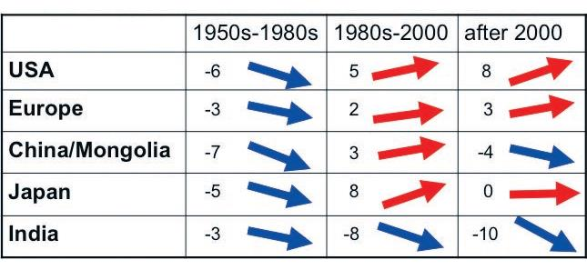
Fig. 1. Qualitative tendencies in decadal SSR changes over theperiods 1950s to 1980s, 1980s to 2000, and post-2000 in different world regions that are well covered by historic SSR records.

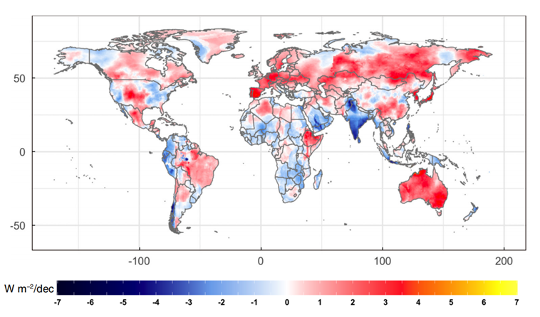
Recent developments include the use of machine learning methods to spatially and temporally augment the limited worldwide in-situ SSR observational records (Yuan et al.,2021; Jiao et al., 2023). These methods generate spatially complete SSR datasets over the entire land surface (Fig. 2). Figure 2 shows some characteristic features of SSR trends during the 1985−2019 “brightening period”, such as the substantial brightening over Europe and the continuous dimming in India. It remains a challenge to fully assess the reliability of the trends of these machine learning-based estimations, particularly in regions that lack the constraints of in-situ radiation observations.

Fig. 2. Worldwide linear trends of the annual average SSR during the “brightening” period of 1985–2019 based on ground observations spatially augmented by machine learning methods [Reprinted from Yuan et al. (2021), © American Meteorological Society. Used with permission.]

Impacts in China

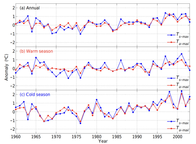
A number of studies have shown that changes in SSR have affected warming rates in China, particularly in terms of the mean and maximum 2-m air temperatures. Daily maximum temperatures were shown to increase less than daily minimum temperatures in China since the 1960s, particularly in the decades of strongest dimming, indicative of a dampening effect of SSR dimming, particularly on the daily maximum temperature warming rates most directly affected by SSR changes (Wang et al., 2012a; Du et al., 2017; Zhao et al., 2021). The evolution of daily maximum land surface (Ts-max) and 2-m air (Ta-max) temperatures averaged over China from the 1960s to 2003 is illustrated in Fig. 5 in terms of their annual means and the means of the warm and cold seasons (from Du et al., 2017).

Fig. 5. China-mean anomalies of daily maximum land surface temperature (Ts-max, blue line) and daily maximum air temperature (Ta-max, red line) for the (a) entire year, (b) warm season (May−October), and (c) cold season (November−April) with respect to the reference period 1961–90,based on 1977 stations [Reprinted from Du et al. (2017).]

Previous Post  Hard Evidence of Solar Impact upon Earth Cloudiness

Later on is a reprinted discussion of global dimming and brightness resulting from fluctuating cloud cover.  This is topical because of new empirical research findings coming out of Asia.  H/T GWPF.  A study published by Kobe University research center is Revealing the impact of cosmic rays on the Earth’s climate.  Excerpts in italics with my bolds.

New evidence suggests that high-energy particles from space known as galactic cosmic rays affect the Earth’s climate by increasing cloud cover, causing an “umbrella effect”.

When galactic cosmic rays increased during the Earth’s last geomagnetic reversal transition 780,000 years ago, the umbrella effect of low-cloud cover led to high atmospheric pressure in Siberia, causing the East Asian winter monsoon to become stronger. This is evidence that galactic cosmic rays influence changes in the Earth’s climate. The findings were made by a research team led by Professor Masayuki Hyodo (Research Center for Inland Seas, Kobe University) and published on June 28 in the online edition of Scientific Reports.

The Svensmark Effect is a hypothesis that galactic cosmic rays induce low cloud formation and influence the Earth’s climate. Tests based on recent meteorological observation data only show minute changes in the amounts of galactic cosmic rays and cloud cover, making it hard to prove this theory. However, during the last geomagnetic reversal transition, when the amount of galactic cosmic rays increased dramatically, there was also a large increase in cloud cover, so it should be possible to detect the impact of cosmic rays on climate at a higher sensitivity.

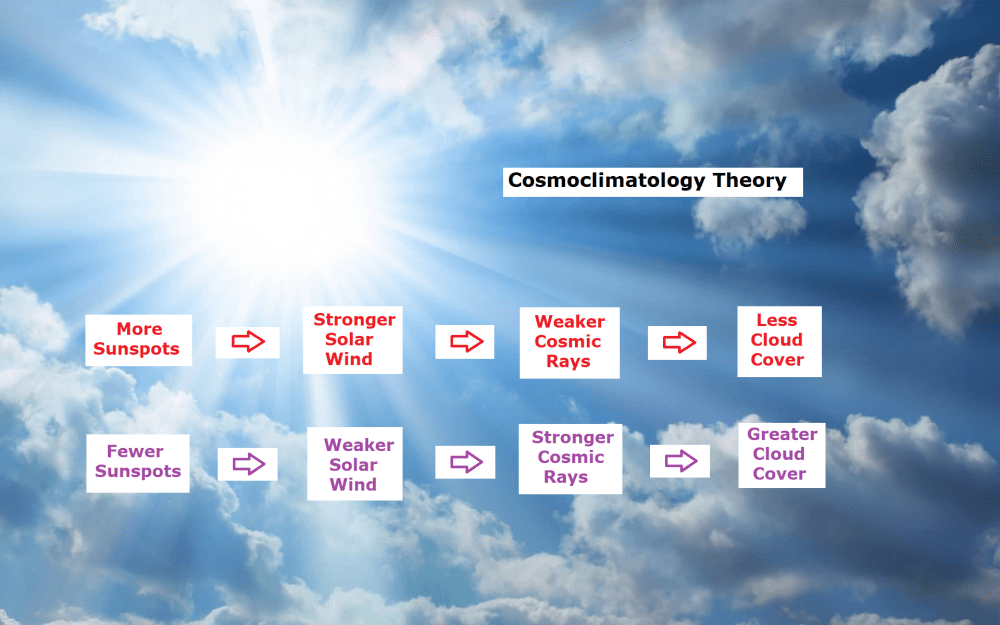
(The Svenmark Effect is explained in essay The cosmoclimatology theory)

How Nature’s Sunscreen Works (from Previous Post)

A recent post Planetary Warming: Back to Basics discussed a recent paper by Nikolov and Zeller on the atmospheric thermal effect measured on various planets in our solar system. They mentioned that an important source of temperature variation around the earth’s energy balance state can be traced to global brightening and dimming.

This post explores the fact of fluctuations in the amount of solar energy reflected rather than absorbed by the atmosphere and surface. Brightening refers to more incoming solar energy from clear and clean skies. Dimming refers to less solar energy due to more sunlight reflected in the atmosphere by the presence of clouds and aerosols (air-born particles like dust and smoke).

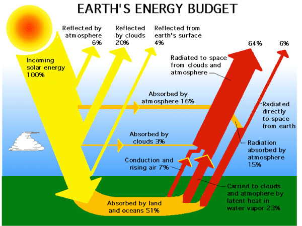
The energy budget above from ERBE shows how important is this issue. On average, half of sunlight is either absorbed in the atmosphere or reflected before it can be absorbed by the surface land and ocean. Any shift in the reflectivity (albedo) impacts greatly on the solar energy warming the planet.

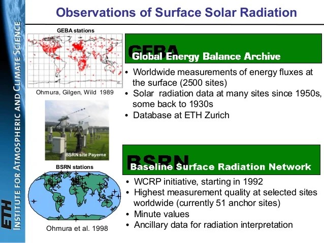
The leading research on global brightening/dimming is done at
the Institute for Atmospheric and Climate Science of ETH Zurich,
led by Dr. Martin Wild, senior scientist specializing in the subject.

Special instruments have been recording the solar radiation that reaches the Earth’s surface since 1923. However, it wasn’t until the International Geophysical Year in 1957/58 that a global measurement network began to take shape. The data thus obtained reveal that the energy provided by the sun at the Earth’s surface has undergone considerable variations over the past decades, with associated impacts on climate.

The initial studies were published in the late 1980s and early 1990s for specific regions of the Earth. In 1998 the first global study was conducted for larger areas, like the continents Africa, Asia, North America and Europe for instance.

Now ETH has announced The Global Energy Balance Archive (GEBA) version 2017: A database for worldwide measured surface energy fluxes. The title is a link to that paper published in May 2017 explaining the facility and some principal findings. The Archive itself is at  http://www.geba.ethz.ch.

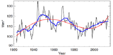
For example, Figure 2 below provides the longest continuous record available in GEBA: surface downward shortwave radiation measured in Stockholm since 1922. Five year moving average in blue, 4th order regression model in red. Units Wm-2. Substantial multidecadal variations become evident, with an increase up to the 1950s (“early brightening”), an overall decline from the 1950s to the 1980s (“dimming”), and a recovery thereafter (“brightening”).
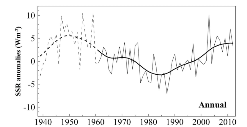
Figure 5. Composite of 56 European GEBA time series of annual surface downward shortwave radiation (thin line) from 1939 to 2013, plotted together with a 21 year Gaussian low-pass filter ((thick line). The series are expressed as anomalies (in Wm-2) from the 1971–2000 mean. Dashed lines are used prior to 1961 due to the lower number of records for this initial period. Updated from Sanchez-Lorenzo et al. (2015) including data until December 2013.
Martin Wild explains in a 2016 article Decadal changes in radiative fluxes at land and ocean surfaces and their relevance for global warming. From the Conclusion (SSR refers to solar radiation incident upon the surface)

However, observations indicate not only changes in the downward thermal fluxes, but even more so in their solar counterparts, whose records have a much wider spatial and temporal coverage. These records suggest multidecadal variations in SSR at widespread land-based observation sites. Specifically, declining tendencies in SSR between the 1950s and 1980s have been found at most of the measurement sites (‘dimming’), with a partial recovery at many of the sites thereafter (‘brightening’).

With the additional information from more widely measured meteorological quantities which can serve as proxies for SSR (primarily sunshine duration and DTR), more evidence for a widespread extent of these variations has been provided, as well as additional indications for an overall increasing tendency in SSR in the first part of the 20th century (‘early brightening’).

It is well established that these SSR variations are not caused by variations in the output of the sun itself, but rather by variations in the transparency of the atmosphere for solar radiation. It is still debated, however, to what extent the two major modulators of the atmospheric transparency, i.e., aerosol and clouds, contribute to the SSR variations.

The balance of evidence suggests that on longer (multidecadal) timescales aerosol changes dominate, whereas on shorter (decadal to subdecadal) timescales cloud effects dominate. More evidence is further provided for an increasing influence of aerosols during the course of the 20th century. However, aerosol and clouds may also interact, and these interactions were hypothesized to have the potential to amplify and dampen SSR trends in pristine and polluted areas, respectively.

No direct observational records are available over ocean surfaces. Nevertheless, based on the presented conceptual ideas of SSR trends amplified by aerosol–cloud interactions over the pristine oceans, modeling approaches as well as the available satellite-derived records it appears plausible that also over oceans significant decadal changes in SSR occur.

The coinciding multidecadal variations in SSTs and global aerosol emissions may be seen as a smoking gun, yet it is currently an open debate to what extent these SST variations are forced by aerosol-induced changes in SSR, effectively amplified by aerosol– cloud interactions, or are merely a result of unforced natural variations in the coupled ocean atmosphere system. Resolving this question could state a major step toward a better understanding of multidecadal climate change.

Another paper co-authored by Wild discusses the effects of aerosols and clouds The solar dimming/brightening effect over the Mediterranean Basin in the period 1979 − 2012. (NSWR is Net Short Wave Radiation, that is equal to surface solar radiation less reflected)

The analysis reveals an overall increasing trend in NSWR (all skies) corresponding to a slight solar brightening over the region (+0.36 Wm−2per decade), which is not statistically significant at 95% confidence level (C.L.). An increasing trend(+0.52 Wm−2per decade) is also shown for NSWR under clean skies (without aerosols), which is statistically significant (P=0.04).

This indicates that NSWR increases at a higher rate over the Mediterranean due to cloud variations only, because of a declining trend in COD (Cloud Optical Depth). The peaks in NSWR (all skies) in certain years (e.g., 2000) are attributed to a significant decrease in COD (see Figs. 9 and 10), whilethe two data series (NSWRall and NSWRclean) are highly correlated(r=0.95).

This indicates that cloud variation is the major regulatory factor for the amount and multi-decadal trends in NSWR over the Mediterranean Basin. (Note: Lower cloud optical depth is caused by less opaque clouds and/or decrease in overall cloudiness)

On the other hand, the results do not reveal a reversal from dimming to brightening during 1980s, as shown in several studies over Europe (Norris and Wild, 2007;Sanchez-Lorenzoet al., 2015), but a rather steady slight increasing trend in solar radiation, which, however, seems to be stabilized during the last years of the data series, in agreement with Sanchez-Lorenzo et al. (2015). Similarly, Wild (2012) reported that the solar brightening was less distinct at European sites after 2000 compared to the 1990s.

In contrast, the NSWR under clear (cloudless) skies shows a slight but statistically significant decreasing trend (−0.17 Wm−2per decade,P=0.002), indicating an overall decrease in NSWR over the Mediterranean due to water-vapor variability suggesting a transition to more humid environment under a warming climate.

Other researchers find cloudiness more dominant than aerosols. For example, The cause of solar dimming and brightening at the Earth’s surface during the last half century: Evidence from measurements of sunshine duration by Gerald Stanhill et al.

Analysis of the Angstrom-Prescott relationship between normalized values of global radiation and sunshine duration measured during the last 50 years made at five sites with a wide range of climate and aerosol emissions showed few significant differences in atmospheric transmissivity under clear or cloud-covered skies between years when global dimming occurred and years when global brightening was measured, nor in most cases were there any significant changes in the parameters or in their relationships to annual rates of fossil fuel combustion in the surrounding 1° cells. It is concluded that at the sites studied changes in cloud cover rather than anthropogenic aerosols emissions played the major role in determining solar dimming and brightening during the last half century and that there are reasons to suppose that these findings may have wider relevance.

Summary

The final words go to Martin Wild from Enlightening Global Dimming and Brightening.

Observed Tendencies in surface solar radiation
Figure 2.  Changes in surface solar radiation observed in regions with good station coverage during three periods.(left column) The 1950s–1980s show predominant declines (“dimming”), (middle column) the 1980s–2000 indicate partial recoveries (“brightening”) at many locations, except India, and (right column) recent developments after 2000 show mixed tendencies. Numbers denote typical literature estimates for the specified region and period in W m–2 per decade.  Based on various sources as referenced in Wild (2009).

The latest updates on solar radiation changes observed since the new millennium show no globally coherent trends anymore (see above and Fig. 2). While brightening persists to some extent in Europe and the United States, there are indications for a renewed dimming in China associated with the tremendous emission increases there after 2000, as well as unabated dimming in India (Streets et al. 2009; Wild et al. 2009).

We cannot exclude the possibility that we are currently again in a transition phase and may return to a renewed overall dimming for some years to come.

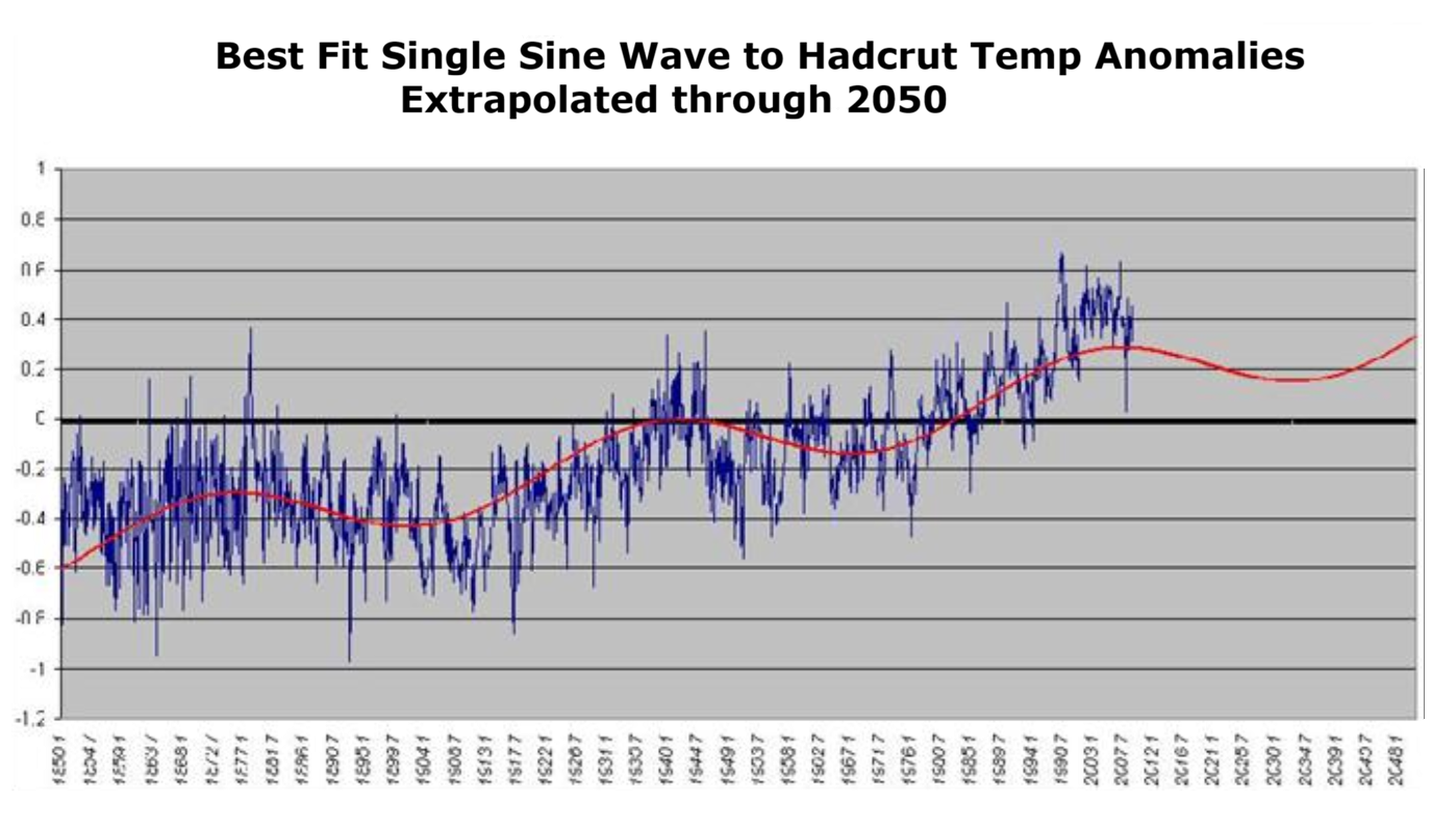
One can’t help but see the similarity between dimming/brightening and patterns of Global Mean Temperature, such as HadCrut.

Footnote: For more on clouds, precipitation and the ocean, see Here Comes the Rain Again

It’s Summertime, Hottest Year Claims Ensue

Matthew Wielicki explains the scientific malpractice in his Financial Post article Junk Science Week: The hottest year ever?.  Excerpts in italics wtih my bolds and added images

Advocates and the media claim 2024 was the hottest year ever.
Archeological data suggest it wasn’t,
while modern data suffer from biases

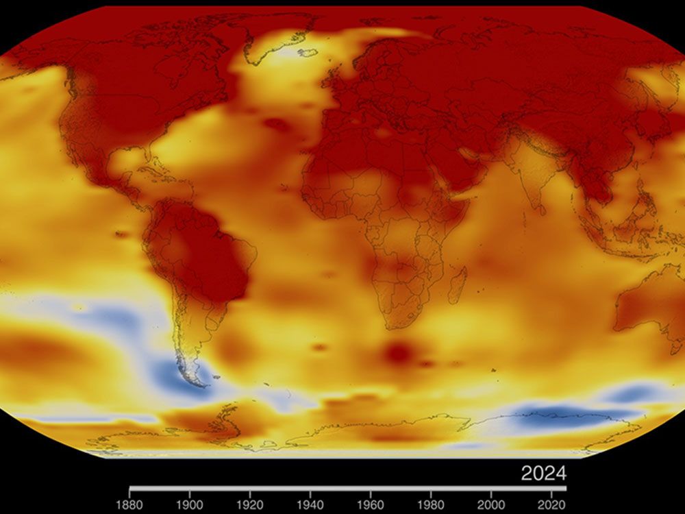
An image produced by NASA and used when it declared 2024 as the warmest year on record. Photo by NASA

In 2024, mainstream media and political leaders aggressively promoted the alarming narrative that Earth had just experienced its hottest year ever recorded. National Geographic dramatically proclaimed, “2024 was the hottest year ever … and the coldest year of the rest of your life,” while the Vancouver Sun declared unequivocally, “Scientists confirm 2024 was Canada’s and world’s hottest year on record.” Canadian political figures reinforced this narrative, with prime minister Justin Trudeau characterizing the year’s warmth as an urgent call for immediate climate action.

I’m an earth science professor-in-exile. Claims such as these
immediately provoke critical skepticism.

This persistent narrative, relentlessly advanced by a powerful climate-industrial complex comprising governments, activist organizations and the media, is designed not merely to inform, but to generate a state of perpetual urgency. As global greenhouse gas (GHG) emissions continue to rise despite decades of climate policy interventions, the need to claim climate conditions are increasingly severe becomes a strategic imperative, regardless of scientific accuracy or historical context. This approach not only distorts genuine scientific inquiry but fosters anxiety and despair, particularly affecting young people already inundated with predictions of catastrophe.

The answers to four fundamental questions expose the weaknesses and biases inherent in the mainstream climate narrative:

1. Can we accurately measure historical global temperatures?

Claims about unprecedented global heat depend heavily on comparing modern temperature records, which are gathered by instrument and capture annual or monthly fluctuations, to historical temperature estimates derived from proxy data such as ice cores, tree rings, sediment layers and coral reefs. But proxy data inherently smooths out short-term fluctuations, providing generalized temperature estimates spanning centuries or millennia. This mismatch between high-resolution modern data and low-resolution historical proxies inevitably exaggerates the perceived severity of contemporary warming.

For example, widely cited reconstructions and favourites of The Intergovernmental Panel on Climate Change (IPCC) explicitly acknowledge their inability to capture temperature variability occurring over periods shorter than 300 years. The rapid temperature changes of recent decades appear unprecedented when put side by side with these smoothed historical averages. This methodological flaw significantly undermines the credibility of claims asserting that current global temperatures are historically unique or alarming.

2. Was 2024 really unprecedentedly warm?

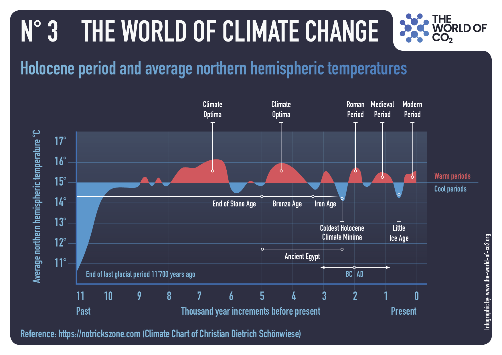
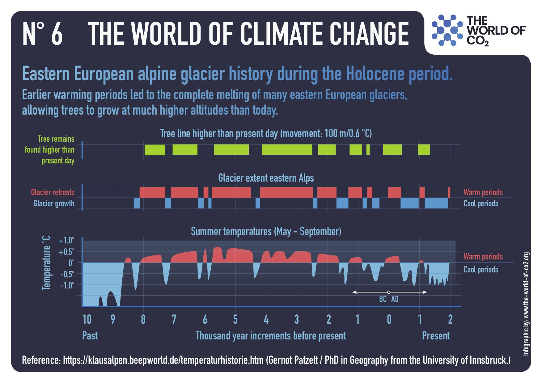
Extensive historical and geological evidence demonstrates significant natural warming vastly exceeding modern temperatures. The Holocene Thermal Maximum (five to nine thousand years ago) saw temperatures significantly warmer than today, including in Canada. Archeological evidence, such as ancient forests revealed by retreating glaciers in the Rockies, conclusively supports periods of substantial natural warmth.

During the Eemian interglacial period (115-130 thousand years ago), Greenland experienced temperatures three to five degrees C warmer than now, despite substantially lower CO₂ concentrations in the atmosphere. These scientifically documented periods confirm that Earth’s climate naturally experiences considerable variability, rendering claims of unprecedented modern warmth scientifically untenable and historically uninformed.

3. Are we measuring the effects of CO₂ or urban heat islands

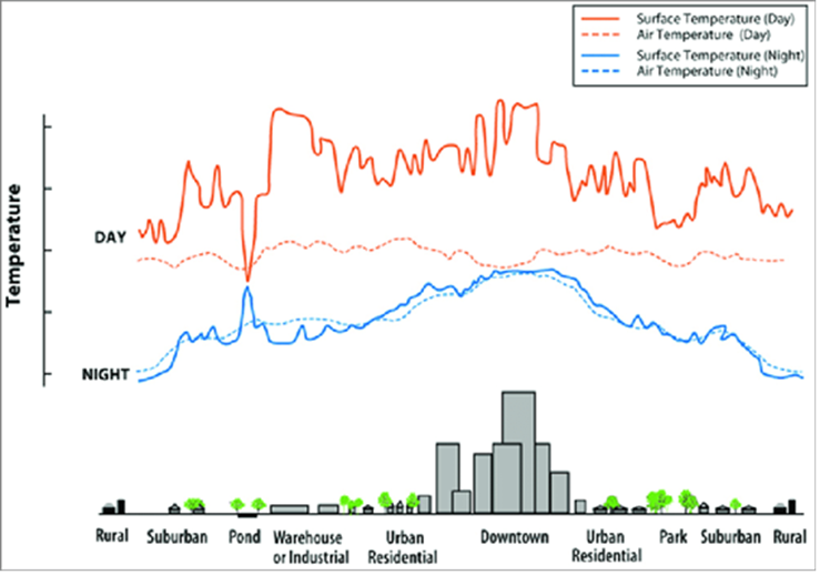
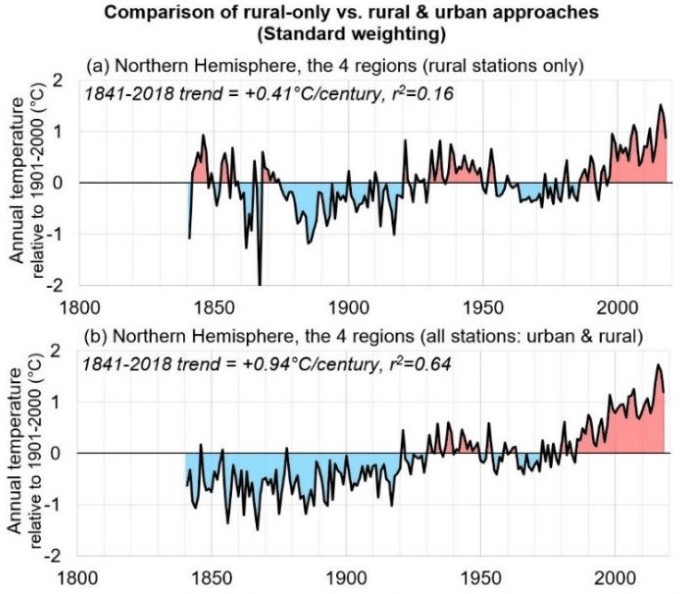
Most modern temperature records fuelling alarmist headlines originate from urban areas influenced by the Urban Heat Island Effect (UHIE). UHIE results from urban infrastructure, such as concrete, asphalt and buildings, retaining and radiating heat, significantly increasing local temperatures independent of broader climate trends. Toronto’s significant infrastructure growth has noticeably raised local temperatures, heavily skewing data. Similarly, Las Vegas’ highest recorded temperatures coincided with significant expansion around Harry Reid International Airport, illustrating the dominant role of urbanization rather than atmospheric CO₂ emissions.

Recent research indicates that up to 65 per cent of urban warming is from local urbanization rather than global greenhouse gas increases. Attributing urban heat predominantly to CO₂ emissions significantly misrepresents the true dynamics of local temperature increases.

4. Do rising CO2 levels really heat the oceans?

Recent alarmist coverage in outlets like the Financial Times highlights near-record ocean temperatures, linking them directly to rising CO₂ levels. The EU’s Copernicus programme noted that May 2025 ocean temperatures were the second highest ever recorded, with scientists raising concerns about the oceans’ diminishing capacity to absorb CO₂ and excess heat.

But this narrative critically overlooks fundamental scientific facts. Oceans possess a heat capacity orders of magnitude greater than the atmosphere. The notion that atmospheric CO₂ significantly heats ocean water directly is scientifically unfounded, as infrared radiation from CO₂ penetrates mere millimetres into the ocean’s surface, not nearly deep enough to meaningfully alter ocean temperature. Ocean temperature fluctuations are primarily driven by natural phenomena such as El Niño.

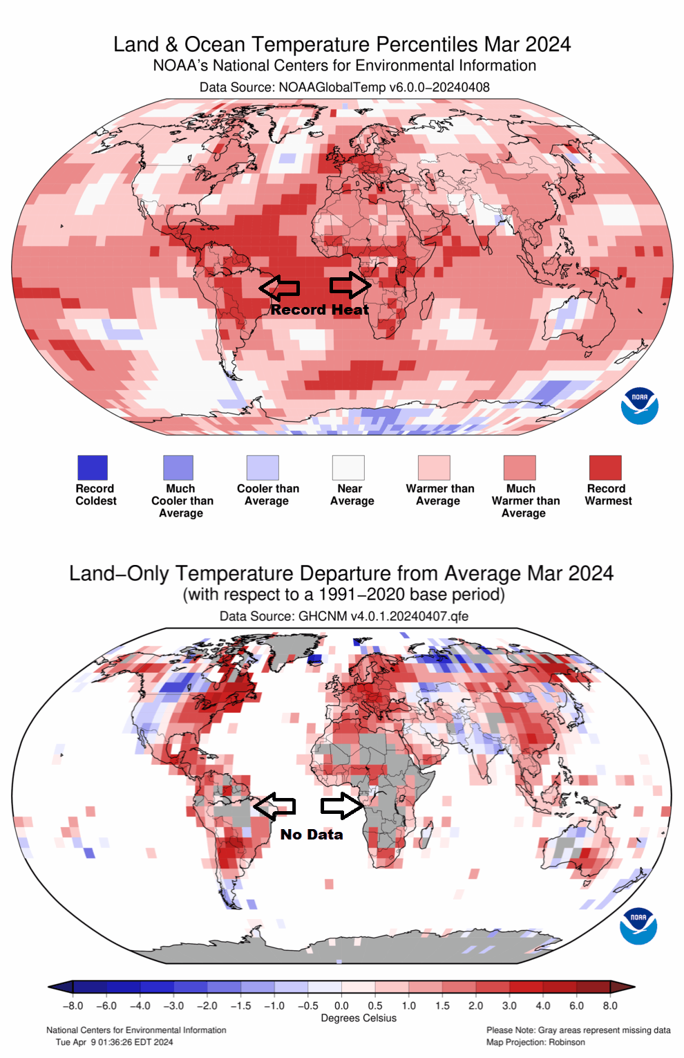
Furthermore, going back to previous warmings prior to the satellite record shows that the entire rise of 0.8C since 1947 is due to oceanic, not human activity.

Moreover, historical data on ocean temperatures is highly uncertain, relying predominantly on sparse measurements and indirect proxies. Claiming near-record ocean temperatures without acknowledging these substantial uncertainties misleads the public about the robustness and reliability of these measurements.

Critical conclusion: One thing remains certain: it will never be “too hot” in Canada, despite alarmist rhetoric suggesting otherwise. The exaggerated claims that 2024 was “the hottest year ever” are not grounded in rigorous scientific analysis but serve primarily as political and ideological propaganda. This relentless propagation of fear fosters anxiety, despair, and nihilism, especially among young people — serious consequences largely ignored by climate alarmists.

The scientific community, policy-makers and the public at large need to insist on transparency, rigour and honesty in climate discourse. Recognizing the motivations behind alarmist claims is essential to ensuring public trust and effective policy. Climate science should strive to educate, not frighten, promoting balanced understanding rather than catastrophic narratives disconnected from historical context and scientific rigour.

Matthew Wielicki, Ph.D. in geochemistry from UCLA, publishes the Substack site Irrational Fear, which provides data-driven critiques aimed at fostering a balanced and scientifically grounded understanding of climate science.

May 2025 Two Years of Ocean Cooling Persists

The best context for understanding decadal temperature changes comes from the world’s sea surface temperatures (SST), for several reasons:
  • The ocean covers 71% of the globe and drives average temperatures;
  • SSTs have a constant water content, (unlike air temperatures), so give a better reading of heat content variations;
  • A major El Nino was the dominant climate feature in recent years.

HadSST is generally regarded as the best of the global SST data sets, and so the temperature story here comes from that source. Previously I used HadSST3 for these reports, but Hadley Centre has made HadSST4 the priority, and v.3 will no longer be updated.  HadSST4 is the same as v.3, except that the older data from ship water intake was re-estimated to be generally lower temperatures than shown in v.3.  The effect is that v.4 has lower average anomalies for the baseline period 1961-1990, thereby showing higher current anomalies than v.3. This analysis concerns more recent time periods and depends on very similar differentials as those from v.3 despite higher absolute anomaly values in v.4.  More on what distinguishes HadSST3 and 4 from other SST products at the end. The user guide for the current version HadSST4.1.1.0 is here.   The charts and analysis below is produced from the current data.

The Current Context

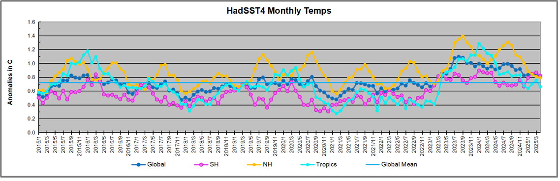
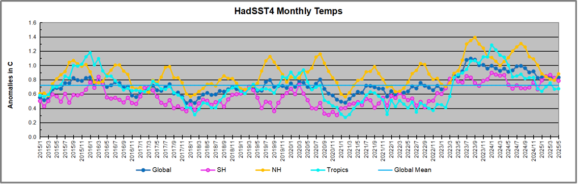
The chart below shows SST monthly anomalies as reported in HadSST4 starting in 2015 through May 2025. A global cooling pattern is seen clearly in the Tropics since its peak in 2016, joined by NH and SH cycling downward since 2016, followed by rising temperatures in 2023 and 2024.

Note that in 2015-2016 the Tropics and SH peaked in between two summer NH spikes.  That pattern repeated in 2019-2020 with a lesser Tropics peak and SH bump, but with higher NH spikes. By end of 2020, cooler SSTs in all regions took the Global anomaly well below the mean for this period.  A small warming was driven by NH summer peaks in 2021-22, but offset by cooling in SH and the tropics, By January 2023 the global anomaly was again below the mean.

Then in 2023-24 came an event resembling 2015-16 with a Tropical spike and two NH spikes alongside, all higher than 2015-16. There was also a coinciding rise in SH, and the Global anomaly was pulled up to 1.1°C last year, ~0.3° higher than the 2015 peak.  Then NH started down autumn 2023, followed by Tropics and SH descending 2024 to the present. After 12 months of cooling in SH and the Tropics, the Global anomaly came back down, led by NH cooling the last 8 months from its 1.3C peak in August, down to 0.8C in March and April.  Remarkably, April 2025 SST anomalies in all regions and globally are the coolest since March 2023.  May shows little change in the Global anomaly, with a SH decline offsetting an upward bump in NH.

Comment:

The climatists have seized on this unusual warming as proof their Zero Carbon agenda is needed, without addressing how impossible it would be for CO2 warming the air to raise ocean temperatures.  It is the ocean that warms the air, not the other way around.  Recently Steven Koonin had this to say about the phonomenon confirmed in the graph above:

El Nino is a phenomenon in the climate system that happens once every four or five years.  Heat builds up in the equatorial Pacific to the west of Indonesia and so on.  Then when enough of it builds up it surges across the Pacific and changes the currents and the winds.  As it surges toward South America it was discovered and named in the 19th century  It iswell understood at this point that the phenomenon has nothing to do with CO2.

Now people talk about changes in that phenomena as a result of CO2 but it’s there in the climate system already and when it happens it influences weather all over the world.   We feel it when it gets rainier in Southern California for example.  So for the last 3 years we have been in the opposite of an El Nino, a La Nina, part of the reason people think the West Coast has been in drought.

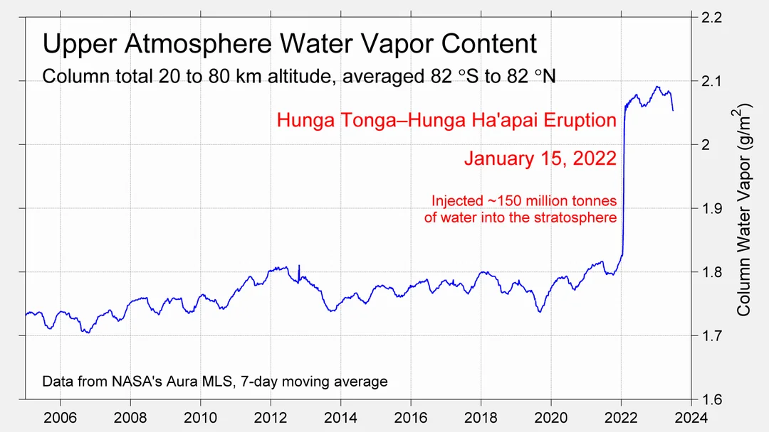
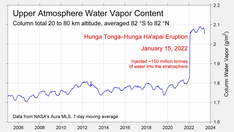
It has now shifted in the last months to an El Nino condition that warms the globe and is thought to contribute to this Spike we have seen. But there are other contributions as well.  One of the most surprising ones is that back in January of 2022 an enormous underwater volcano went off in Tonga and it put up a lot of water vapor into the upper atmosphere. It increased the upper atmosphere of water vapor by about 10 percent, and that’s a warming effect, and it may be that is contributing to why the spike is so high.

A longer view of SSTs

To enlarge image, open in new tab.

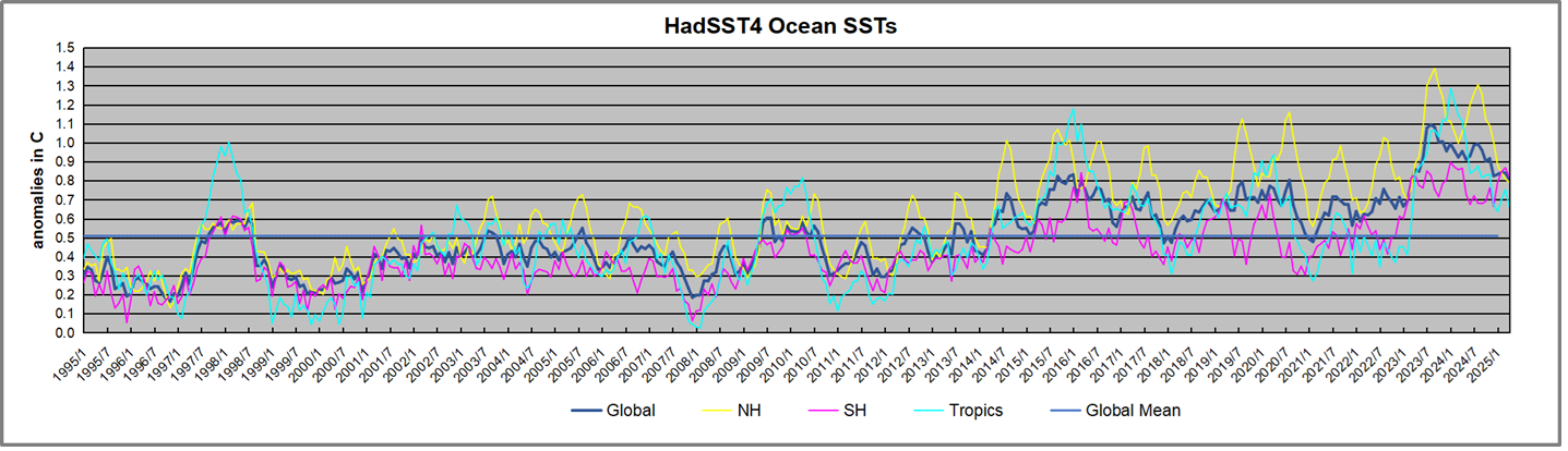
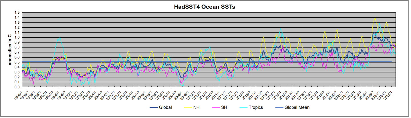
The graph above is noisy, but the density is needed to see the seasonal patterns in the oceanic fluctuations.  Previous posts focused on the rise and fall of the last El Nino starting in 2015.  This post adds a longer view, encompassing the significant 1998 El Nino and since.  The color schemes are retained for Global, Tropics, NH and SH anomalies.  Despite the longer time frame, I have kept the monthly data (rather than yearly averages) because of interesting shifts between January and July. 1995 is a reasonable (ENSO neutral) starting point prior to the first El Nino.

The sharp Tropical rise peaking in 1998 is dominant in the record, starting Jan. ’97 to pull up SSTs uniformly before returning to the same level Jan. ’99. There were strong cool periods before and after the 1998 El Nino event. Then SSTs in all regions returned to the mean in 2001-2.

SSTS fluctuate around the mean until 2007, when another, smaller ENSO event occurs. There is cooling 2007-8,  a lower peak warming in 2009-10, following by cooling in 2011-12.  Again SSTs are average 2013-14.

Now a different pattern appears.  The Tropics cooled sharply to Jan 11, then rise steadily for 4 years to Jan 15, at which point the most recent major El Nino takes off.  But this time in contrast to ’97-’99, the Northern Hemisphere produces peaks every summer pulling up the Global average.  In fact, these NH peaks appear every July starting in 2003, growing stronger to produce 3 massive highs in 2014, 15 and 16.  NH July 2017 was only slightly lower, and a fifth NH peak still lower in Sept. 2018.

The highest summer NH peaks came in 2019 and 2020, only this time the Tropics and SH were offsetting rather adding to the warming. (Note: these are high anomalies on top of the highest absolute temps in the NH.)  Since 2014 SH has played a moderating role, offsetting the NH warming pulses. After September 2020 temps dropped off down until February 2021.  In 2021-22 there were again summer NH spikes, but in 2022 moderated first by cooling Tropics and SH SSTs, then in October to January 2023 by deeper cooling in NH and Tropics.

Then in 2023 the Tropics flipped from below to well above average, while NH produced a summer peak extending into September higher than any previous year.  Despite El Nino driving the Tropics January 2024 anomaly higher than 1998 and 2016 peaks, following months cooled in all regions, and the Tropics continued cooling in April, May and June along with SH dropping.  After July and August NH warming again pulled the global anomaly higher, September through January 2025 resumed cooling in all regions, continuing February through April 2025, with little change in May.

What to make of all this? The patterns suggest that in addition to El Ninos in the Pacific driving the Tropic SSTs, something else is going on in the NH.  The obvious culprit is the North Atlantic, since I have seen this sort of pulsing before.  After reading some papers by David Dilley, I confirmed his observation of Atlantic pulses into the Arctic every 8 to 10 years.

Contemporary AMO Observations

Through January 2023 I depended on the Kaplan AMO Index (not smoothed, not detrended) for N. Atlantic observations. But it is no longer being updated, and NOAA says they don’t know its future.  So I find that ERSSTv5 AMO dataset has current data.  It differs from Kaplan, which reported average absolute temps measured in N. Atlantic.  “ERSST5 AMO  follows Trenberth and Shea (2006) proposal to use the NA region EQ-60°N, 0°-80°W and subtract the global rise of SST 60°S-60°N to obtain a measure of the internal variability, arguing that the effect of external forcing on the North Atlantic should be similar to the effect on the other oceans.”  So the values represent SST anomaly differences between the N. Atlantic and the Global ocean.

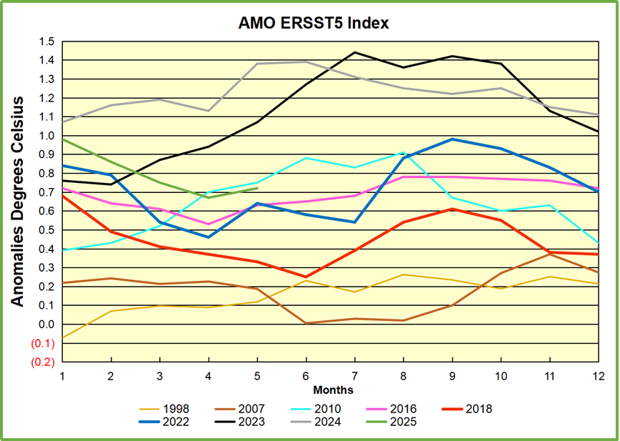
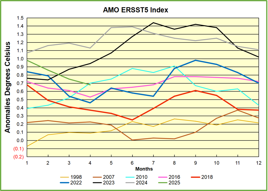
The chart above confirms what Kaplan also showed.  As August is the hottest month for the N. Atlantic, its variability, high and low, drives the annual results for this basin.  Note also the peaks in 2010, lows after 2014, and a rise in 2021. Then in 2023 the peak was holding at 1.4C before declining.  An annual chart below is informative:

Note the difference between blue/green years, beige/brown, and purple/red years.  2010, 2021, 2022 all peaked strongly in August or September.  1998 and 2007 were mildly warm.  2016 and 2018 were matching or cooler than the global average.  2023 started out slightly warm, then rose steadily to an  extraordinary peak in July.  August to October were only slightly lower, but by December cooled by ~0.4C.

Then in 2024 the AMO anomaly started higher than any previous year, then leveled off for two months declining slightly into April.  Remarkably, May showed an upward leap putting this on a higher track than 2023, and rising slightly higher in June.  In July, August and September 2024 the anomaly declined, and despite a small rise in October, ended close to where it began.  Note 2025 started much lower than the previous year and is headed sharply downward, well below the previous two years, now in May aligning with 2010.

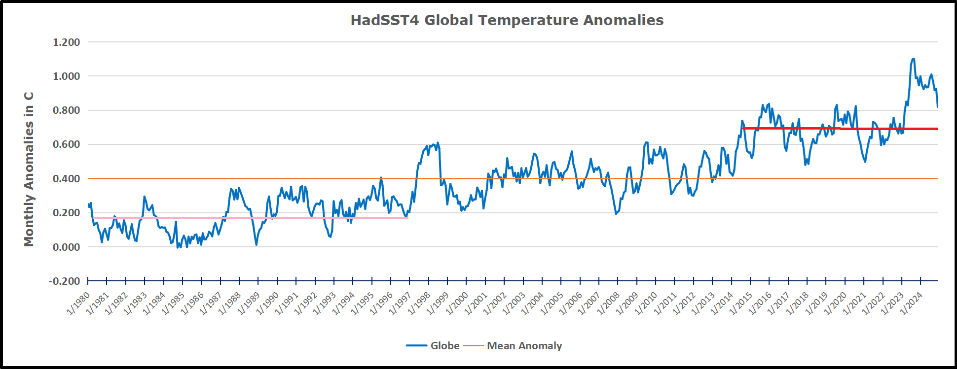
The pattern suggests the ocean may be demonstrating a stairstep pattern like that we have also seen in HadCRUT4.

The purple line is the average anomaly 1980-1996 inclusive, value 0.17.  The orange line the average 1980-2024, value 0.38, also for the period 1997-2012. The red line is 2013-2024, value 0.67. As noted above, these rising stages are driven by the combined warming in the Tropics and NH, including both Pacific and Atlantic basins.

Curiosity:  Solar Coincidence?

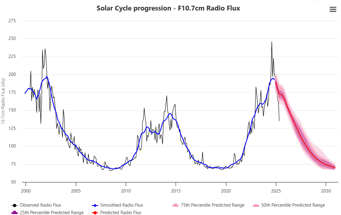
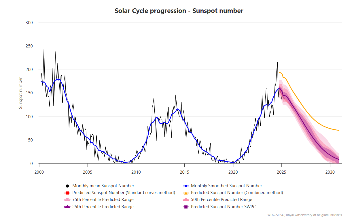
The news about our current solar cycle 25 is that the solar activity is hitting peak numbers now and higher  than expected 1-2 years in the future.  As livescience put it:  Solar maximum could hit us harder and sooner than we thought. How dangerous will the sun’s chaotic peak be?  Some charts from spaceweatherlive look familar to these sea surface temperature charts.

Summary


The oceans are driving the warming this century.  SSTs took a step up with the 1998 El Nino and have stayed there with help from the North Atlantic, and more recently the Pacific northern “Blob.”  The ocean surfaces are releasing a lot of energy, warming the air, but eventually will have a cooling effect.  The decline after 1937 was rapid by comparison, so one wonders: How long can the oceans keep this up? And is the sun adding forcing to this process?

Footnote: Why Rely on HadSST4

HadSST is distinguished from other SST products because HadCRU (Hadley Climatic Research Unit) does not engage in SST interpolation, i.e. infilling estimated anomalies into grid cells lacking sufficient sampling in a given month. From reading the documentation and from queries to Met Office, this is their procedure.

HadSST4 imports data from gridcells containing ocean, excluding land cells. From past records, they have calculated daily and monthly average readings for each grid cell for the period 1961 to 1990. Those temperatures form the baseline from which anomalies are calculated.

In a given month, each gridcell with sufficient sampling is averaged for the month and then the baseline value for that cell and that month is subtracted, resulting in the monthly anomaly for that cell. All cells with monthly anomalies are averaged to produce global, hemispheric and tropical anomalies for the month, based on the cells in those locations. For example, Tropics averages include ocean grid cells lying between latitudes 20N and 20S.

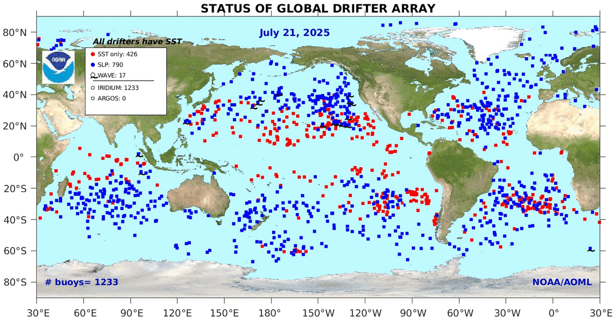
Gridcells lacking sufficient sampling that month are left out of the averaging, and the uncertainty from such missing data is estimated. IMO that is more reasonable than inventing data to infill. And it seems that the Global Drifter Array displayed in the top image is providing more uniform coverage of the oceans than in the past.

uss-pearl-harbor-deploys-global-drifter-buoys-in-pacific-ocean

USS Pearl Harbor deploys Global Drifter Buoys in Pacific Ocean

Meet Téa Johansson, Teenage Climate Realist

For those who prefer reading, below is a transcript lightly edited from the closed captions with my bolds along with some of the exhibits and added images.

Life on Earth is in crisis crop failure, social and ecological collapse, mass extinction.  We have a moral duty to take action.  These statements made by Extinction Rebellion reflect the climate alarmist narrative that has continued to escalate across the Western world.  Hysteria over climate change can be seen throughout history, from the human sacrifices of the Aztecs to bring back rain, to the Salem witch trials to eliminate the women they blamed for crop failure during the little ice age.

Today the climate industrial complex is funded by trillions of dollars seeking to control what we buy, eat and where we are allowed to travel,  all in the name of sustainability and achieving net zero carbon emissions.  This fear campaign is rooted in the belief that we will not look into the data ourselves, but instead look to the governments and to the media to tell us what is true.

Today I will demonstrate that temperatures fluctuate and are not unprecedented, and that natural disasters are not getting worse. I will also highlight the unreliability of climate data and the role of CO2.  Ultimately I will present scientific evidence to show that we are not in a climate crisis.

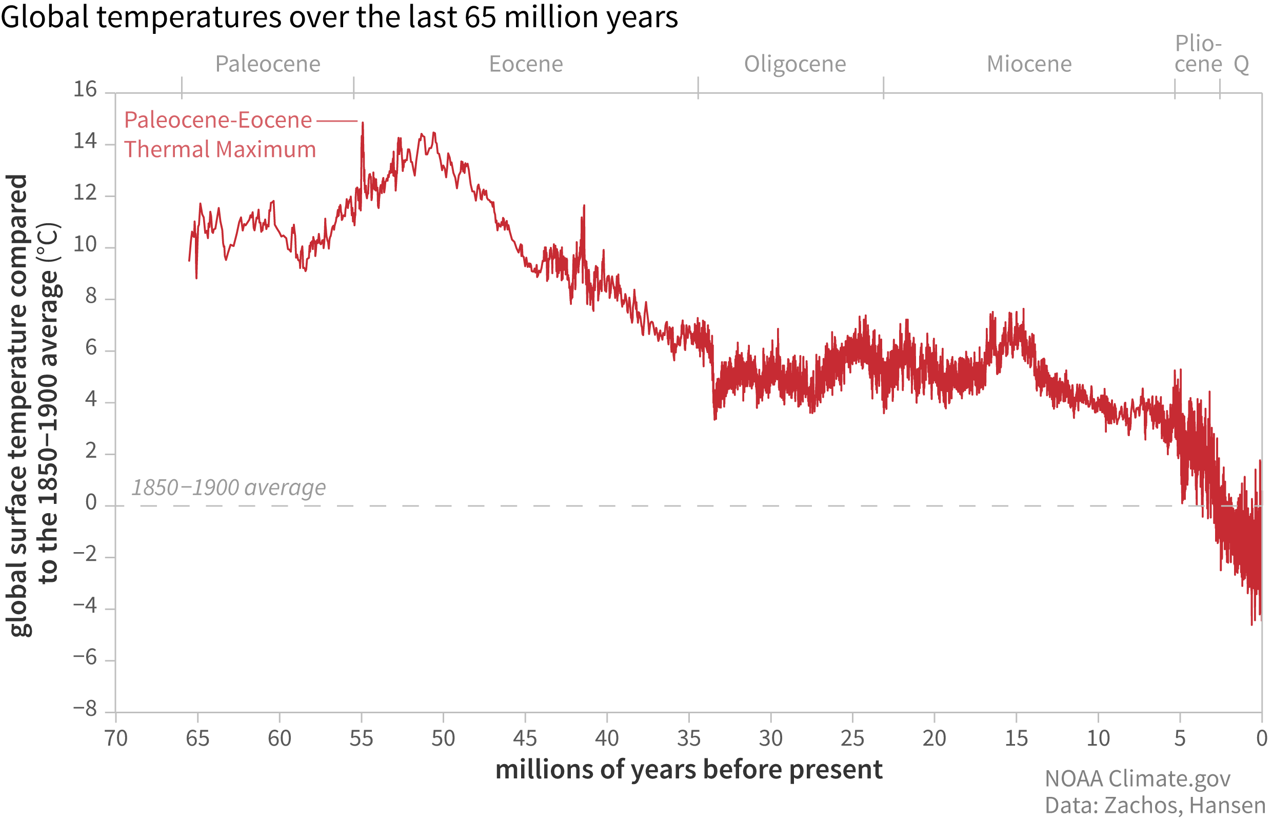
Historical temperature records indicate that we are not in the climate crisis western governments claim.  We are looking at a graph of the past 65 million years from NOAA.  The Earth today seems to be in a particularly cool period; in fact the Earth is still coming out of an ice age. History demonstrates that life has existed and thrived in much warmer temperatures, and that temperatures have been much higher without the human influence of industrial CO2 emissions.  

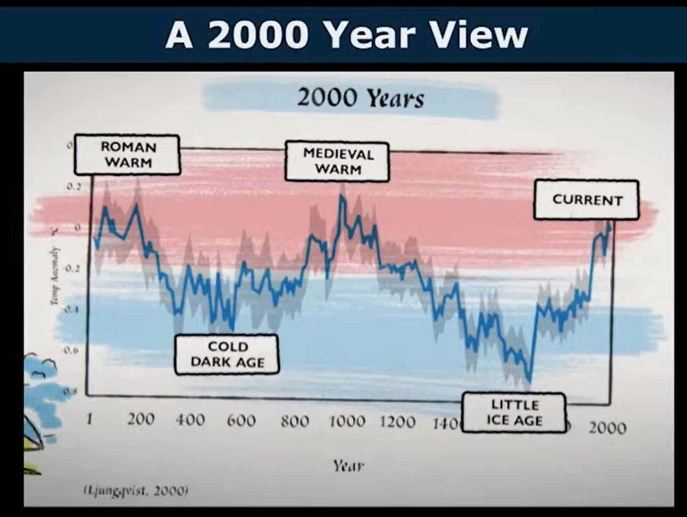
Historical temperature records indicate that the temperature of the Earth naturally fluctuates over time as it has for the past 65 million years.  In just the past 2,000 years there have been two warm periods and two cold periods.  The Roman warm period, also called the Roman optimum, was known as a time of prosperity.  This of course goes against the entire narrative that warming threatens human life.  Following the Roman warm period came the cold dark age,  the medieval warm period, and the Little Ice Age.  The current warming from 1800 onwards is the warming of recovery from the Little Ice Age.  However temperatures are still cold compared to distant times and continue to visibly fluctuate.  

Given this evidence,  the claim by scientists and news pundits that 3° Fahrenheit is the end of civilization is not cause for alarm.  Because it is not unprecedented and because temperatures will continue to fluctuate today.  The argument for climate change is rooted in the belief that warmer weather and CO2 emissions have been causing natural disasters to become more frequent and more violent.   However after studying hurricane and wildfire data, it became clear that actual activity goes against this global warming narrative.

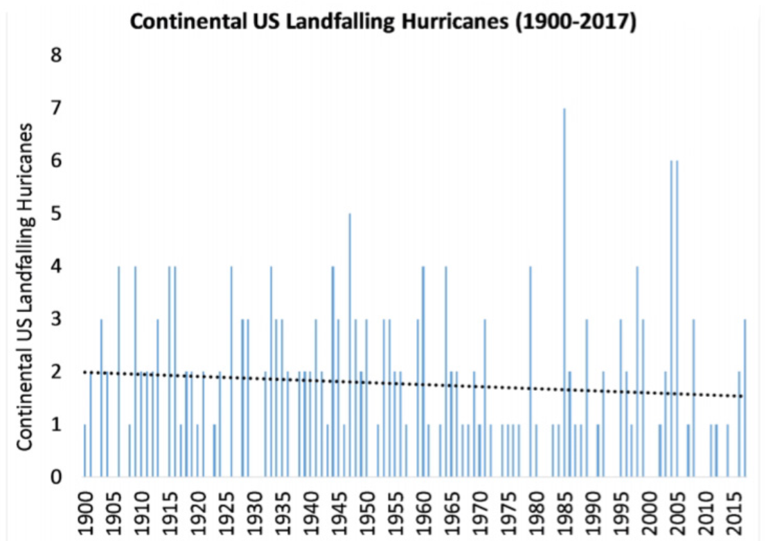
This graph from the bulletin of the American Meteorological Society shows the number of hurricanes in the US per year since 1900 showing a slight downward trend for the past 120 years.  The strength and duration of hurricanes shows a similar lack of crisis.  

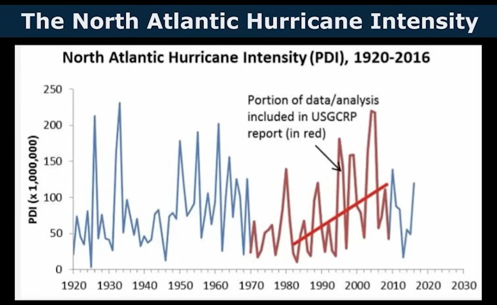
A graph from the National Hurricane Research Laboratory illustrates the North Atlantic hurricane intensity from 1920 to 2016, where there is evidently no trend. However the data presented to the public by the 2014 National Climate Assessment of the United States is limited to the portion highlighted in red creating an illusory upward trend.

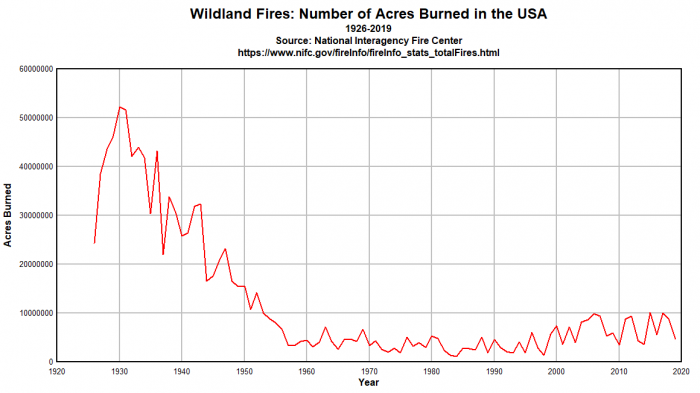
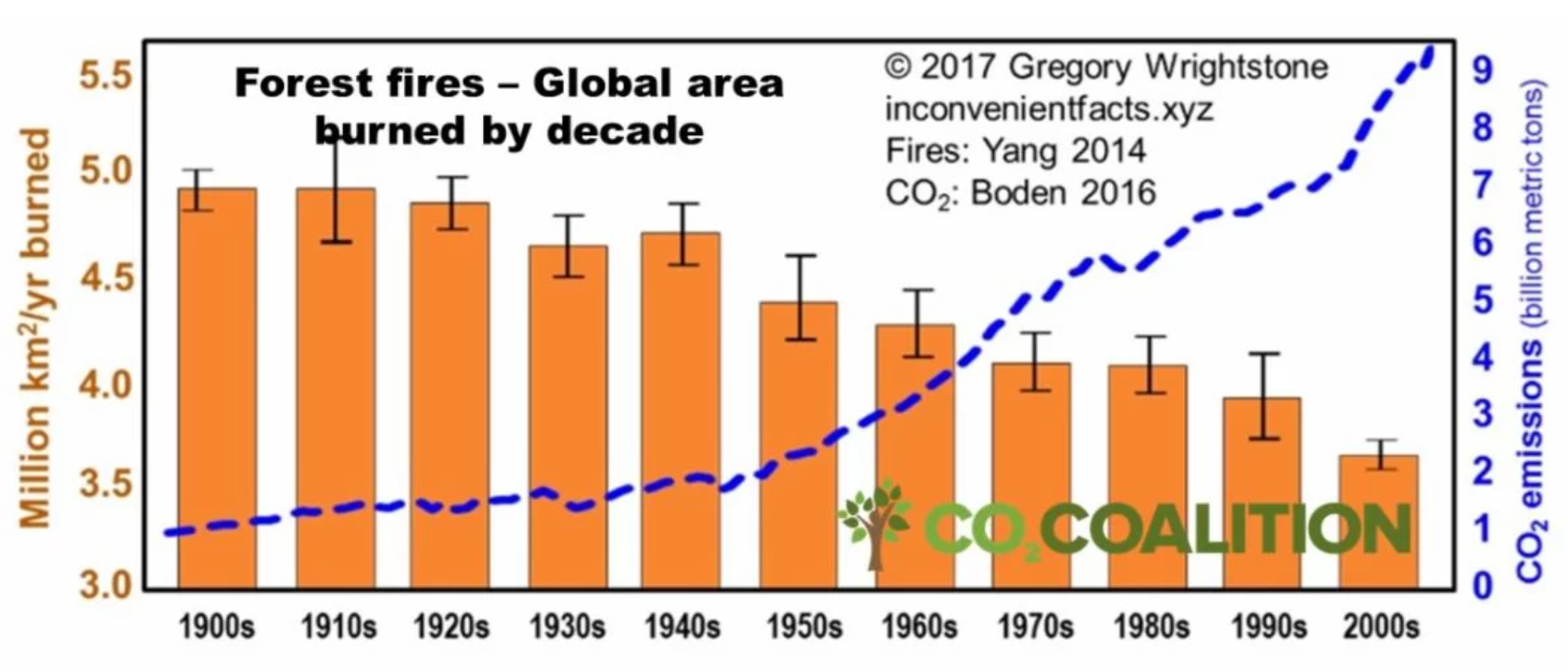
This graph starting in 1920 shows that the number of acres burned by wildfires in the US has been decreasing.  Similarly the number of acres burned globally since 1900 has steadily declined as well. Ultimately the presented evidence goes against the narrative that anthropogenic CO2 emissions have been making the weather worse.

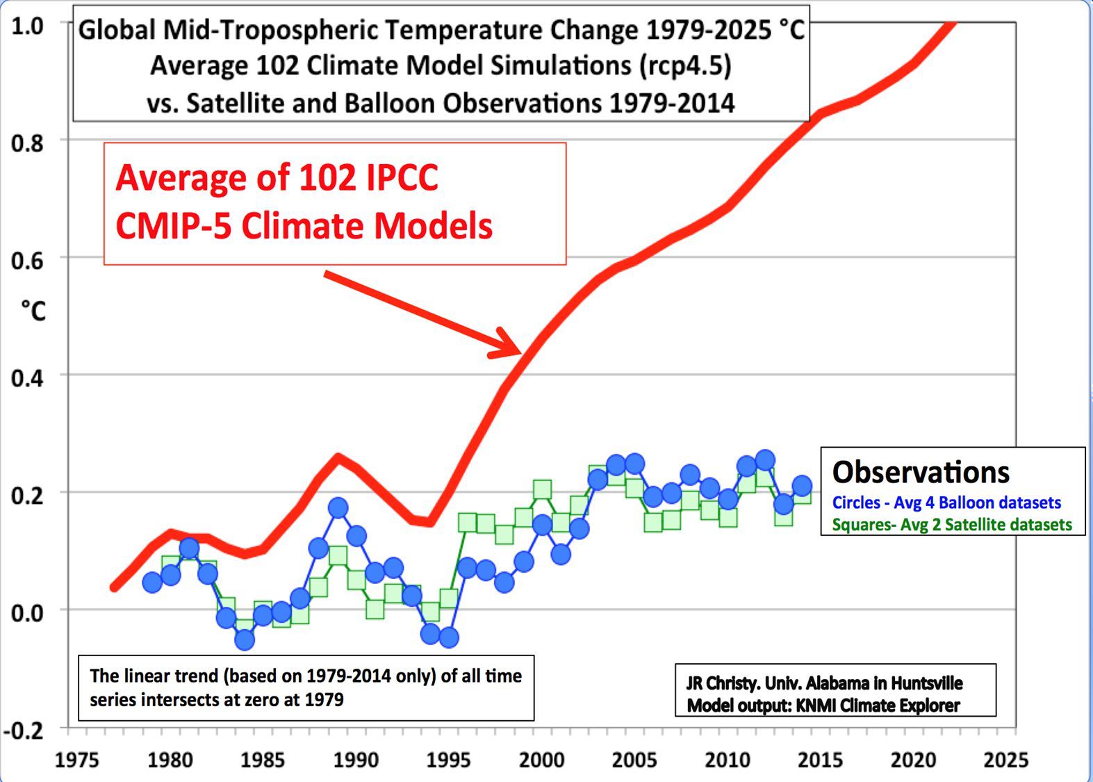
To understand the science behind the climate crisis claims of today, it is necessary to highlight the unreliability of available data.  This is most evident in the disparity between climate model predictions and the observed data.  In this graph illustrating temperature change, the blue line representing data taken from weather balloons matches up well with the green line showing data taken from satellites. However the red line represents the climate models used by the UNIPCC to predict future global warming.  These observations show that actual warming is about one third of that predicted.

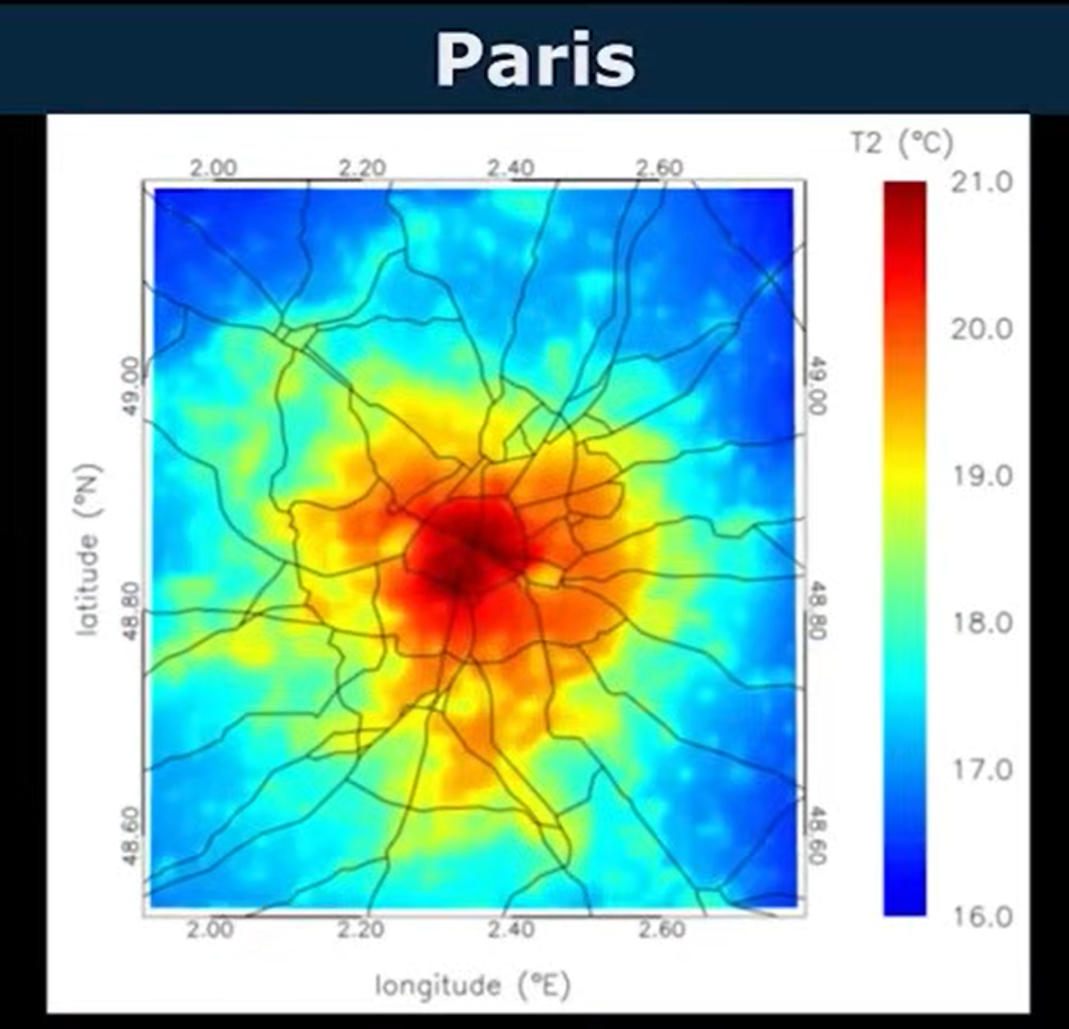
Temperature measurements are greatly affected by what is called the urban heat island effect.  Since concrete picks up heat, temperatures taken in cities are much higher than those taken in rural areas.  For example in a thermal radiation map of the city of Paris, the middle of the city produces a deep red color representing heat, while the rural areas around the city project a green to bluecolor representing milder temperatures.  

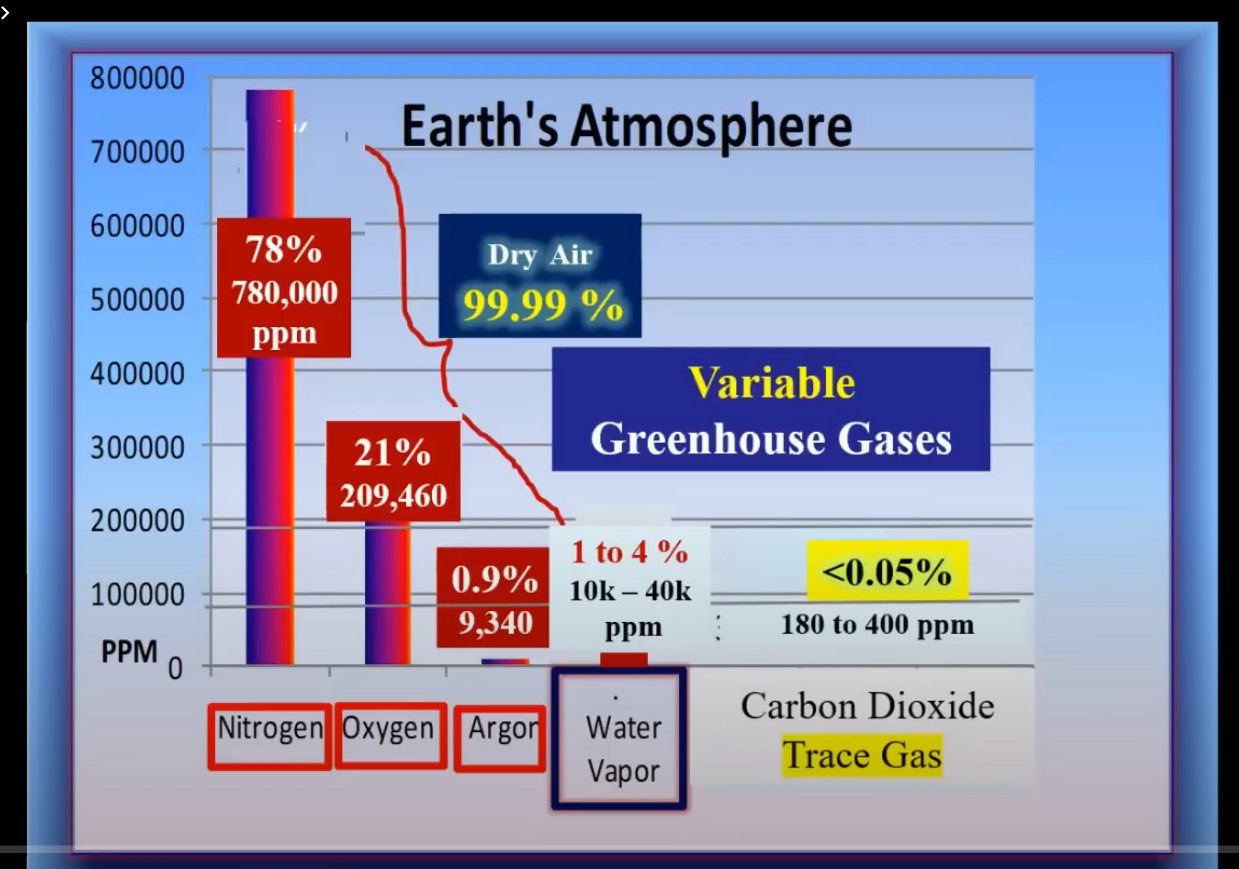
This gap represents one way that climate alarmists can instill fear by embellishing data to serve their agenda. Perhaps the greatest tool of the climate industrial complex is the supposed evil of CO2.  However CO2 is not the control knob for climate change mainly because it is only 0.04% of the atmosphere.  I’ll say it again:  CO2 is only 0.04% of the atmosphere.  A visual comparison of CO2 to the other atmospheric gases shows how barely negligible is the gas in comparison.  

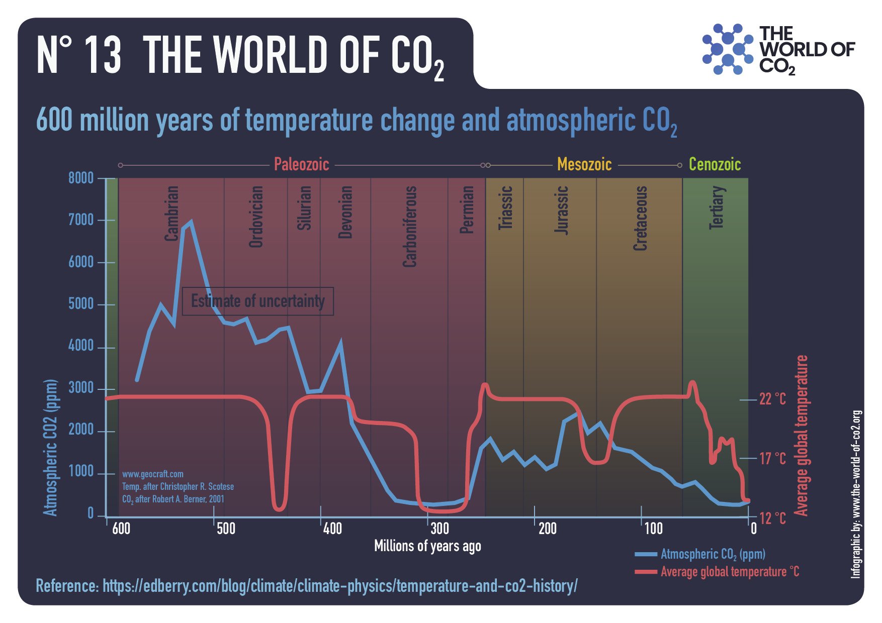
Although the mainstream media has tried to alarm its consumers with the accelerating emissions of CO2, the Earth is actually in a CO2 famine.  Current levels are about 423 parts per million; however in the past they have been at least a thousand parts per million and have likely reached 8,000 parts per million.

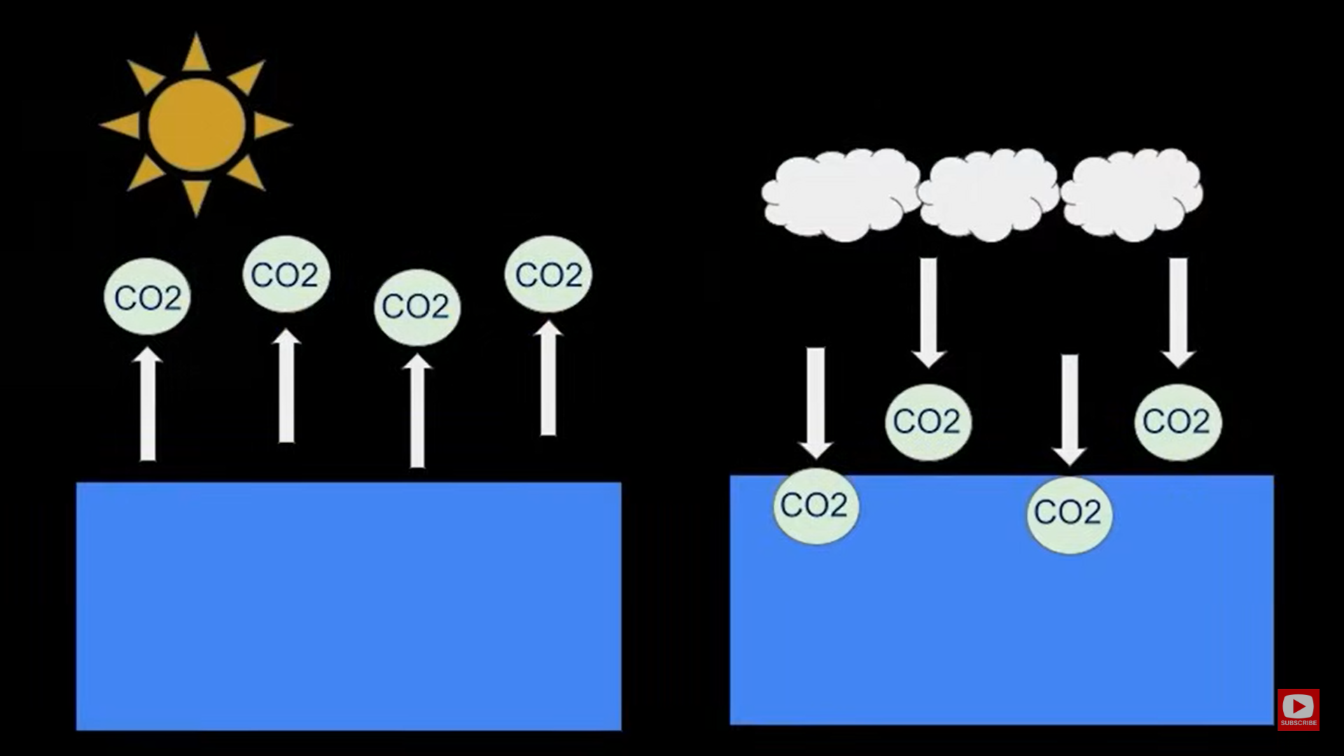
While the narrative states that CO2 directly causes the rise in temperature, it has been found that quite the opposite is true.  The relationship between CO2 and temperature is not that more CO2 causes a rise in temperature, but that a rise in temperature causes an increase in CO2.   Carl Wunsch, professor of oceanography at MIT, found that when the ocean warms more CO2 is released into the atmosphere.  On the other hand when the ocean is cold, CO2 is absorbed into the water.  

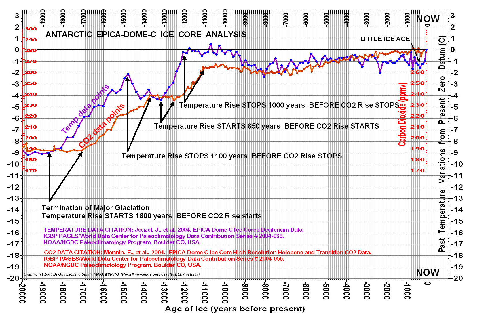
In a graphical correlation between temperature and CO2, it is found that when a rise in temperature occurs, a rise in CO2 follows a few centuries later.  In this graph CO2 rose 800 years later in response to a surge in temperature.

Like everything else in the world, CO2 may have some small factor in climate, while there are countless of other factors affecting temperature.  Some examples are volcanic activity, cosmic rays, and the sun.  This highlights how if we were to limit CO2,  it would only stunt biodiversity while having almost no effect on temperature.  Because of the fact that it is only one small factor in a sea of greater causes.

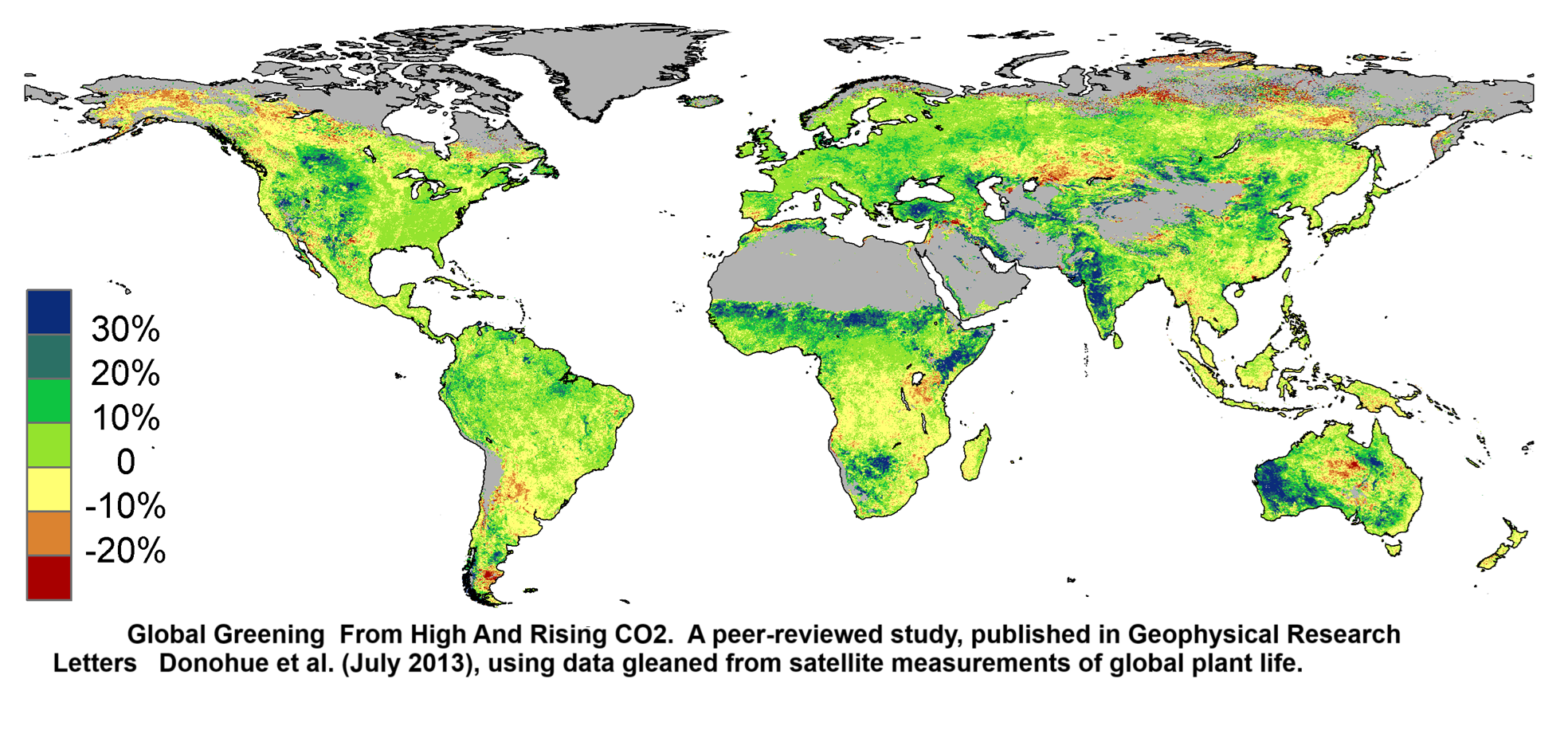
Some call CO2 the gas of life because it plays an instrumental role in the process of photosynthesis. It comes as no surprise that most farmers use high levels of it in their green houses to produce a better crop.  In this picture four pine trees are shown growing at different levels of added CO2, from normal atmospheric CO2 to an added 150, 300, and eventually 450 parts per million.  More CO2 is evidently beneficial for plant growth.  Physicist Lubos Motl, former professor at Harvard, summarized the importance of CO2, saying “It is the key compound that plants need to grow, and indirectly every organism needs to have food.  At the end it is clear that CO2 is not, as the New York Times frighteningly put it, a tiny bit of arsenic or cobra venom.   Nor will it cause famine as many claim; if CO2 increases it will only green the planet and increase the food supply.

Across the western world climate change has been coined as an existential threat to mankind.  While this sentiment is not new over the course of history, as it can be seen through the Aztecs and even in the Salem witch trials.  It has once again become relevant in today’s culture with policies such as carbon taxes and individual CO2 budgets being proposed in our governments.  We are seeing the climate issue creep into every part of our lives.

This is why I I found it necessary to pursue the truth and the climate debate.  In my speech I presented the scientific evidence behind historical temperature change and natural disasters,  discovering the unreliability of climate data, the small role of CO2 in climate, and its essential role in biodiversity.   As a result I’ve concluded that the climate crisis is a hoax that we must arm ourselves against by pursuing the truth and by looking into the data ourselves.

NH and Tropics Lead UAH Temps Lower May 2025

The post below updates the UAH record of air temperatures over land and ocean. Each month and year exposes again the growing disconnect between the real world and the Zero Carbon zealots.  It is as though the anti-hydrocarbon band wagon hopes to drown out the data contradicting their justification for the Great Energy Transition.  Yes, there was warming from an El Nino buildup coincidental with North Atlantic warming, but no basis to blame it on CO2.

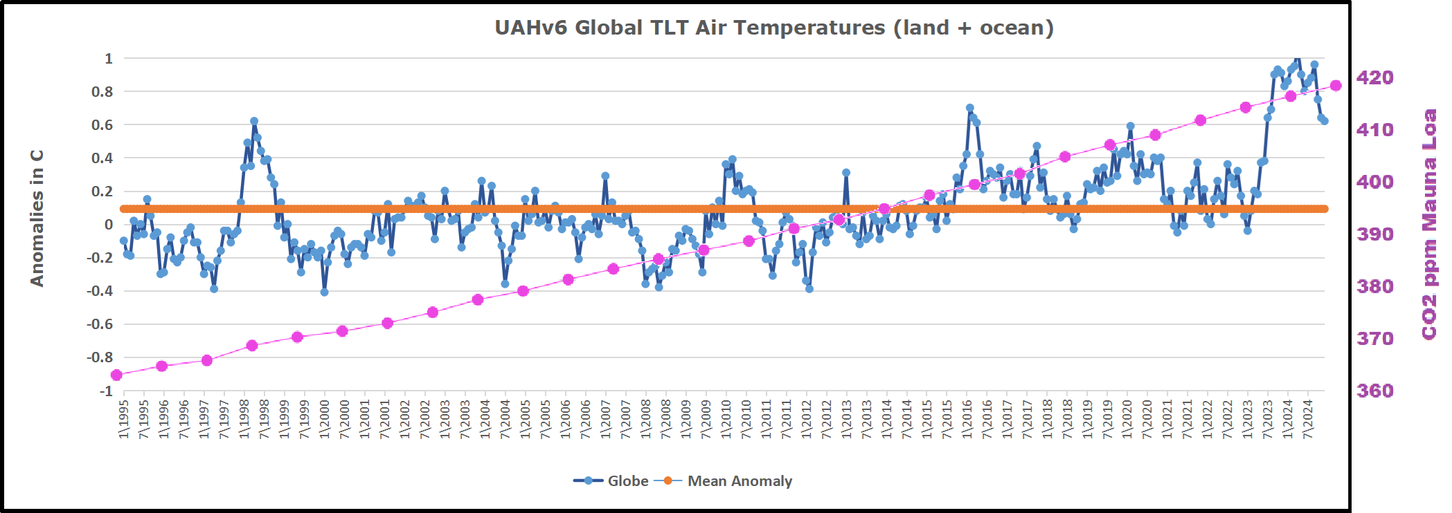
As an overview consider how recent rapid cooling  completely overcame the warming from the last 3 El Ninos (1998, 2010 and 2016).  The UAH record shows that the effects of the last one were gone as of April 2021, again in November 2021, and in February and June 2022  At year end 2022 and continuing into 2023 global temp anomaly matched or went lower than average since 1995, an ENSO neutral year. (UAH baseline is now 1991-2020). Then there was an usual El Nino warming spike of uncertain cause, unrelated to steadily rising CO2 and now dropping steadily.

For reference I added an overlay of CO2 annual concentrations as measured at Mauna Loa.  While temperatures fluctuated up and down ending flat, CO2 went up steadily by ~60 ppm, a 15% increase.

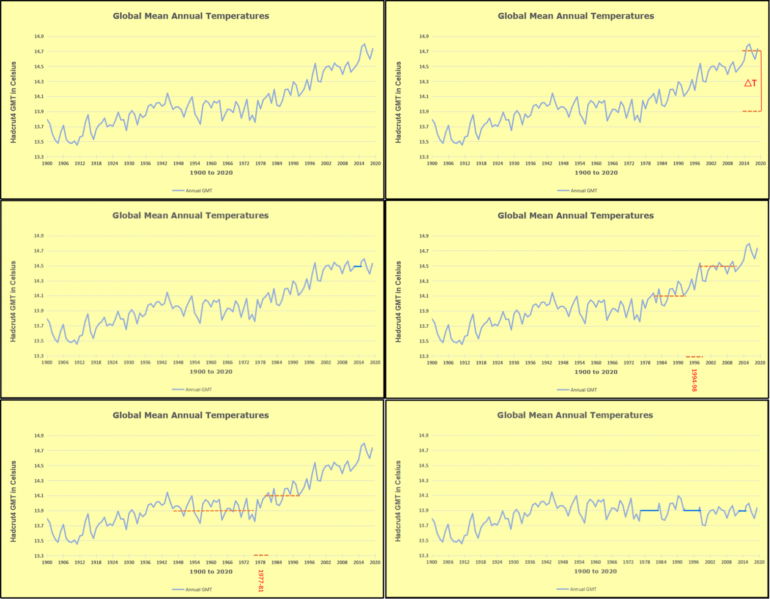
Furthermore, going back to previous warmings prior to the satellite record shows that the entire rise of 0.8C since 1947 is due to oceanic, not human activity.

gmt-warming-events

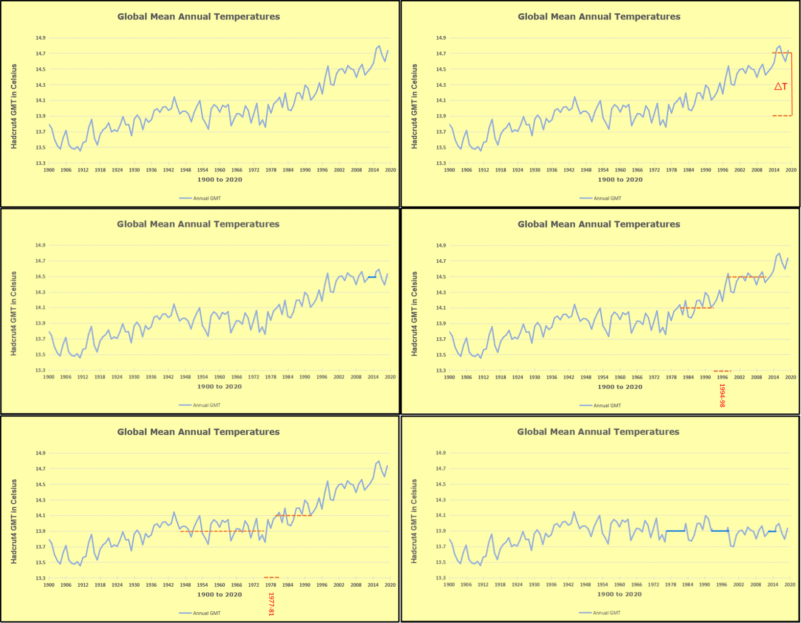
The animation is an update of a previous analysis from Dr. Murry Salby.  These graphs use Hadcrut4 and include the 2016 El Nino warming event.  The exhibit shows since 1947 GMT warmed by 0.8 C, from 13.9 to 14.7, as estimated by Hadcrut4.  This resulted from three natural warming events involving ocean cycles. The most recent rise 2013-16 lifted temperatures by 0.2C.  Previously the 1997-98 El Nino produced a plateau increase of 0.4C.  Before that, a rise from 1977-81 added 0.2C to start the warming since 1947.

Importantly, the theory of human-caused global warming asserts that increasing CO2 in the atmosphere changes the baseline and causes systemic warming in our climate.  On the contrary, all of the warming since 1947 was episodic, coming from three brief events associated with oceanic cycles. And in 2024 we saw an amazing episode with a temperature spike driven by ocean air warming in all regions, along with rising NH land temperatures, now dropping below its peak.

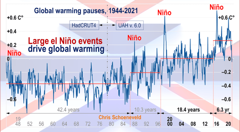
Chris Schoeneveld has produced a similar graph to the animation above, with a temperature series combining HadCRUT4 and UAH6. H/T WUWT

image-8

See Also Worst Threat: Greenhouse Gas or Quiet Sun?

May 2025 NH and Tropics Lead UAH Temps Lower banner-blog

With apologies to Paul Revere, this post is on the lookout for cooler weather with an eye on both the Land and the Sea.  While you heard a lot about 2020-21 temperatures matching 2016 as the highest ever, that spin ignores how fast the cooling set in.  The UAH data analyzed below shows that warming from the last El Nino had fully dissipated with chilly temperatures in all regions. After a warming blip in 2022, land and ocean temps dropped again with 2023 starting below the mean since 1995.  Spring and Summer 2023 saw a series of warmings, continuing into 2024 peaking in April, then cooling off to the present.

UAH has updated their TLT (temperatures in lower troposphere) dataset for May 2025. Due to one satellite drifting more than can be corrected, the dataset has been recalibrated and retitled as version 6.1 Graphs here contain this updated 6.1 data.  Posts on their reading of ocean air temps this month are ahead of the update from HadSST4.  I posted recently on SSTs April 2025 Two Years Ocean Warming Gone These posts have a separate graph of land air temps because the comparisons and contrasts are interesting as we contemplate possible cooling in coming months and years.

Sometimes air temps over land diverge from ocean air changes. In July 2024 all oceans were unchanged except for Tropical warming, while all land regions rose slightly. In August we saw a warming leap in SH land, slight Land cooling elsewhere, a dip in Tropical Ocean temp and slightly elsewhere.  September showed a dramatic drop in SH land, overcome by a greater NH land increase. 2025 has shown a sharp contrast between land and sea, first with ocean air temps falling in January recovering in February.  Then land air temps, especially NH, dropped in February and recovered in March. Now in May both land and sea temps are down in NH and Tropics, overwhelming slight rises of both in SH.

Note:  UAH has shifted their baseline from 1981-2010 to 1991-2020 beginning with January 2021.   v6.1 data was recalibrated also starting with 2021. In the charts below, the trends and fluctuations remain the same but the anomaly values changed with the baseline reference shift.

Presently sea surface temperatures (SST) are the best available indicator of heat content gained or lost from earth’s climate system.  Enthalpy is the thermodynamic term for total heat content in a system, and humidity differences in air parcels affect enthalpy.  Measuring water temperature directly avoids distorted impressions from air measurements.  In addition, ocean covers 71% of the planet surface and thus dominates surface temperature estimates.  Eventually we will likely have reliable means of recording water temperatures at depth.

Recently, Dr. Ole Humlum reported from his research that air temperatures lag 2-3 months behind changes in SST.  Thus cooling oceans portend cooling land air temperatures to follow.  He also observed that changes in CO2 atmospheric concentrations lag behind SST by 11-12 months.  This latter point is addressed in a previous post Who to Blame for Rising CO2?

After a change in priorities, updates are now exclusive to HadSST4.  For comparison we can also look at lower troposphere temperatures (TLT) from UAHv6.1 which are now posted for May 2025.  The temperature record is derived from microwave sounding units (MSU) on board satellites like the one pictured above. Recently there was a change in UAH processing of satellite drift corrections, including dropping one platform which can no longer be corrected. The graphs below are taken from the revised and current dataset.

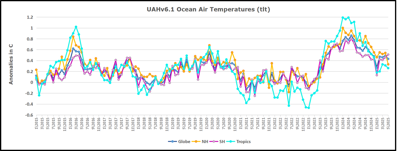
The UAH dataset includes temperature results for air above the oceans, and thus should be most comparable to the SSTs. There is the additional feature that ocean air temps avoid Urban Heat Islands (UHI).  The graph below shows monthly anomalies for ocean air temps since January 2015.

In 2021-22, SH and NH showed spikes up and down while the Tropics cooled dramatically, with some ups and downs, but hitting a new low in January 2023. At that point all regions were more or less in negative territory.

After sharp cooling everywhere in January 2023, there was a remarkable spiking of Tropical ocean temps from -0.5C up to + 1.2C in January 2024.  The rise was matched by other regions in 2024, such that the Global anomaly peaked at 0.86C in April. Since then all regions have cooled down sharply to a low of 0.27C in January.  In February 2025, SH rose from 0.1C to 0.4C pulling the Global ocean air anomaly up to 0.47C, where it stayed in March and April. Now in May drops in NH and Tropics pulled the air temps over oceans down despite an uptick in SH. At 0.43C, ocean air temps are similar to May 2020, albeit with higher SH anomalies.

Land Air Temperatures Tracking in Seesaw Pattern

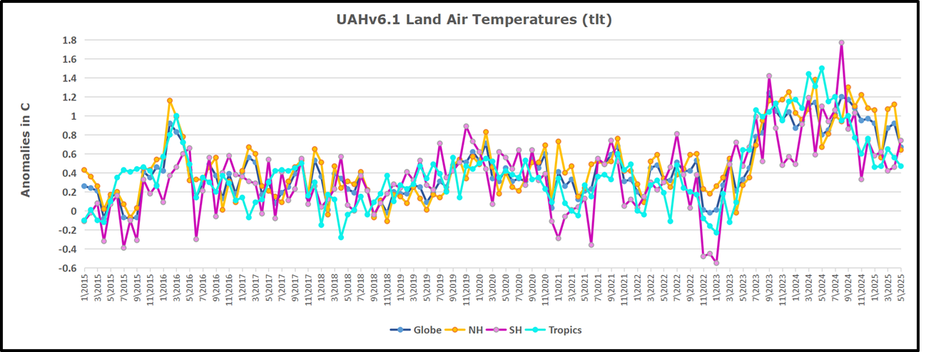
We sometimes overlook that in climate temperature records, while the oceans are measured directly with SSTs, land temps are measured only indirectly.  The land temperature records at surface stations sample air temps at 2 meters above ground.  UAH gives tlt anomalies for air over land separately from ocean air temps.  The graph updated for May is below.

 Here we have fresh evidence of the greater volatility of the Land temperatures, along with extraordinary departures by SH land.  The seesaw pattern in Land temps is similar to ocean temps 2021-22, except that SH is the outlier, hitting bottom in January 2023. Then exceptionally SH goes from -0.6C up to 1.4C in September 2023 and 1.8C in  August 2024, with a large drop in between.  In November, SH and the Tropics pulled the Global Land anomaly further down despite a bump in NH land temps. February showed a sharp drop in NH land air temps from 1.07C down to 0.56C, pulling the Global land anomaly downward from 0.9C to 0.6C. In March that drop reversed with both NH and Global land back to January values, holding there in April.  Now in May, sharp drops in NH and Tropics land air temps pulled the Global land air temps back down close to February value.

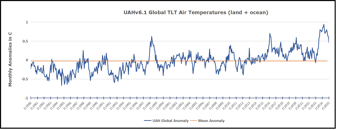
The Bigger Picture UAH Global Since 1980

The chart shows monthly Global Land and Ocean anomalies starting 01/1980 to present.  The average monthly anomaly is -0.03, for this period of more than four decades.  The graph shows the 1998 El Nino after which the mean resumed, and again after the smaller 2010 event. The 2016 El Nino matched 1998 peak and in addition NH after effects lasted longer, followed by the NH warming 2019-20.   An upward bump in 2021 was reversed with temps having returned close to the mean as of 2/2022.  March and April brought warmer Global temps, later reversed

With the sharp drops in Nov., Dec. and January 2023 temps, there was no increase over 1980. Then in 2023 the buildup to the October/November peak exceeded the sharp April peak of the El Nino 1998 event. It also surpassed the February peak in 2016. In 2024 March and April took the Global anomaly to a new peak of 0.94C.  The cool down started with May dropping to 0.9C, and in June a further decline to 0.8C.  October went down to 0.7C,  November and December dropped to 0.6C. February went down to 0.5C, then back up to 0.6C in March and April driven by the bounce in NH land air temps, followed by May’s return to 0.5C.

The graph reminds of another chart showing the abrupt ejection of humid air from Hunga Tonga eruption.

Note on Ocean Cooling Not Yet Fully Appearing in UAH Dataset

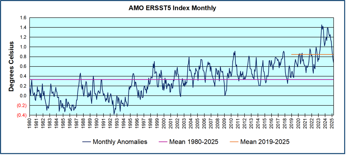
The above chart shows sea surface temperature anomalies (SSTA)  in the North Atlantic 0 to 60N.  The index is derived from ERSSTv.5 by subtracting the global anomalies from the North Atlantic anomalies, the differences as shown in the chart. The baseline of  0.0C is the average for the years 1951 to 1980.  The mean anomaly since 1980 is in purple at 0.33C, and persisted throughout up to 2018. The orange line is the average anomaly in the the last six years, 2019 to 04/2025 inclusive, at 0.84C. The remarkable spikes in 2023 and 2024 drove that rise to exceed 1.4C, which has been cut in half over the last 10 months.  As Dr. Humlum observed, such oceanic changes usually portend air temperature changes later on.

TLTs include mixing above the oceans and probably some influence from nearby more volatile land temps.  Clearly NH and Global land temps have been dropping in a seesaw pattern, nearly 1C lower than the 2016 peak.  Since the ocean has 1000 times the heat capacity as the atmosphere, that cooling is a significant driving force.  TLT measures started the recent cooling later than SSTs from HadSST4, but are now showing the same pattern. Despite the three El Ninos, their warming had not persisted prior to 2023, and without them it would probably have cooled since 1995.  Of course, the future has not yet been written.

Our Atmospheric Heat Engine

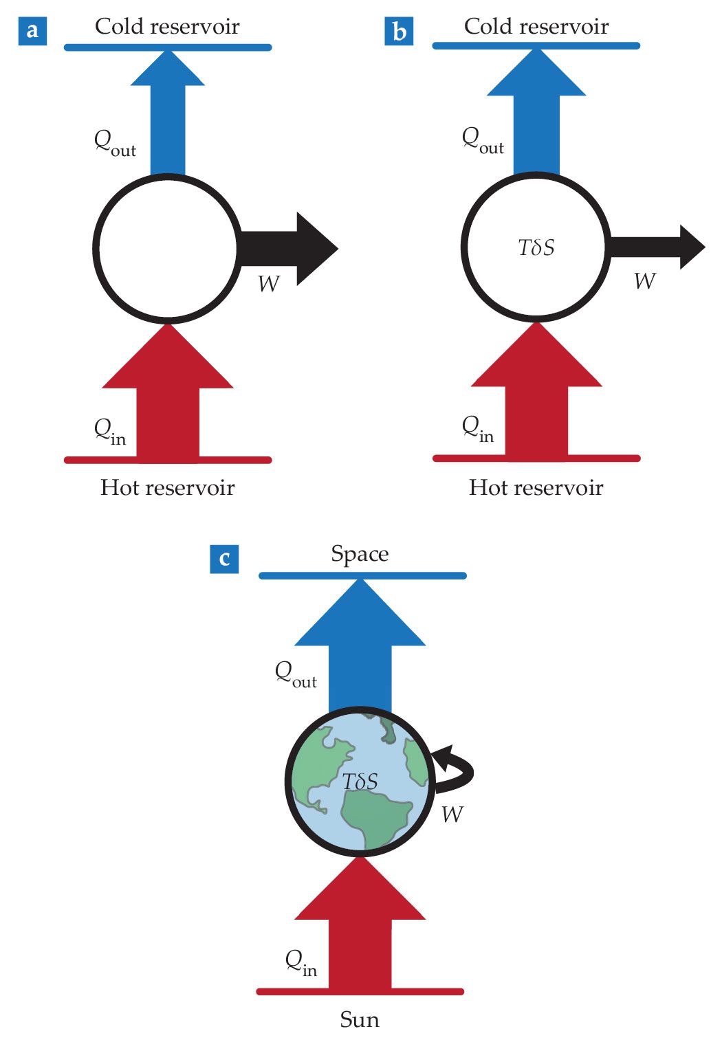
Climate as heat engine. A heat engine produces mechanical energy in the form of work W by absorbing an amount of heat Qin from a hot reservoir (the source) and depositing a smaller amount Qout into a cold reservoir (the sink). (a) An ideal Carnot heat engine does the job with the maximum possible efficiency. (b) Real heat engines are irreversible, and some work is lost via irreversible entropy production TδS. (c) For the climate system, the ultimate source is the Sun, with outer space acting as the sink. The work is performed internally and produces winds and ocean currents. As a result, Qin = Qout.

A previous post presented Michel Thizon’s description of gravity’s effect on the mass of air functioning as a climate thermostat. Some years ago Dr. Murry Salby wrote in detail about the troposphere operating as an heat engine and the stratosphere as a refrigerator. This post consists of excerpts from Salby’s textbook entitled Physics of the Atmosphere and Climate. The title is a link to pdf version of the book Salby (2012). Text in italics with my bolds and added images.

A closed system that performs work through a conversion of heat that is absorbed by it is a heat engine. Conversely, a system that rejects heat through a conversion of work that is performed on it is a refrigerator. In Chap. 6, we will see that individual air parcels comprising the circulation of the troposphere behave as a heat engine.  By absorbing heat at the Earth’s surface, through transfers of radiative, sensible, and latent heat, individual parcels perform net work as they evolve through a thermodynamic cycle (2.13). Ultimately realized as kinetic energy, the heat absorbed maintains the circulation against frictional dissipation. It makes the circulation of the troposphere thermally driven.

In contrast, the circulation of the stratosphere behaves as a radiative refrigerator.  For motion to occur, individual air parcels must have work performed on them. The kinetic energy produced is eventually converted to heat and rejected to space through LW cooling. It makes the circulation of the stratosphere mechanically driven. Gravity waves and planetary waves that propagate upward from the troposphere are dissipated in the stratosphere. Their absorption exerts an influence on the stratosphere analogous to paddle work. By forcing motion that rearranges air, it drives the stratospheric circulation out of radiative equilibrium, which results in net LW cooling to space. Salby (2012) p. 83.

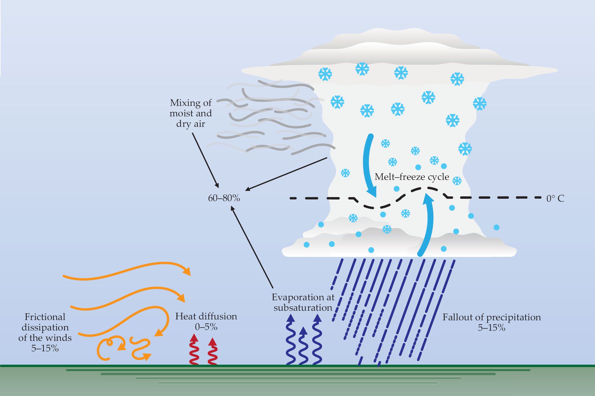
Irreversible processes in the atmosphere. Neglecting radiative processes (not shown here), the largest sources of irreversibility in the atmosphere are those associated with the hydrologic cycle: evaporation, the mixing of moist and dry air, and the melt–freeze cycle (60–80% collectively), and the fallout of precipitation (5–15%). Those contributions limit the entropy generated by frictional dissipation of the winds (5–15%), which ultimately places a limit on the work performed by the atmospheric heat engine in generating circulations. Percentages are estimated based on global climate simulations12 and idealized high-resolution simulations.8

Changes of thermodynamic state that accompany vertical motion follow from the distribution of atmospheric mass, which is determined ultimately by gravity. In the absence of motion, Newton’s second law applied to the vertical reduces to a statement of hydrostatic equilibrium (1.16). Gravity is then balanced by the vertical pressure gradient force. This simple form of mechanical equilibrium is accurate even in the presence of motion because the acceleration of gravity is, almost invariably, much greater than vertical acceleration of individual air parcels. Only inside deep convective towers and other small-scale phenomena is vertical acceleration large enough to invalidate hydrostatic equilibrium.

Because it is such a strong body force, gravity must be treated with some care. Complications arise from the fact that the gravitational acceleration experienced by an air parcel does not act purely in the vertical. It also varies with location. According to the preceding discussion, gravity is large enough to overwhelm other contributions in the balance of vertical forces. The same holds for the balance of horizontal forces. Horizontal components of gravity that are introduced by the Earth’s rotation and other sources must be balanced by additional horizontal forces. Unrelated to air motion, those additional forces unnecessarily complicate the description of atmospheric motion.  Salby (2012) p. 150.

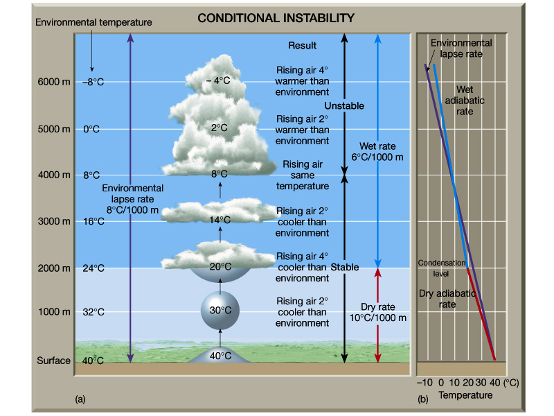
The temperature of a dry air parcel decreases with its altitude at the dry adiabatic lapse rate. To a good approximation, the same holds for a moist air parcel under unsaturated conditions – because the trace abundance of water vapor modifies thermal properties of air only slightly. Under saturated conditions, the adiabatic description of air breaks down due to the release of latent heat that accompanies the transformation of water from one phase to another. Latent heat exchanged with the gas phase then offsets adiabatic cooling and warming, which accompany ascending and descending motion. Salby (2012) p. 162

Net heat absorption and work performed by individual air parcels make the general circulation of the troposphere behave as a heat engine, one that is driven thermally by heat transfer at its lower and upper boundaries. Work performed by individual parcels is associated with a redistribution of mass: Air that is effectively warmer and lighter at the lower boundary is exchanged with air that is effectively cooler and heavier at the upper boundary. This redistribution of mass represents a conversion of potential energy into kinetic energy. The conversion of energy maintains the general circulation against frictional dissipation. Salby (2012) p. 163

The idealized behavior just described relies on heat transfer being confined to the lower and upper boundaries of the layer, where an air parcel resides long enough for diabatic influences to become important. Between the boundaries, the time scale of motion is short. For motion that operates on longer time scales, typical of the stratosphere, the evolution of an individual air parcel is not adiabatic.

Radiative transfer is the primary diabatic influence outside the boundary layer and cloud. It is characterized by cooling rates of order 1 K day−1 in the troposphere (see Fig. 8.24). Cooling rates as large as 10 K day−1 occur in the stratosphere and near cloud (Fig. 9.36). (2012) p. 164

Unlike the troposphere, buoyancy in the stratosphere opposes vertical motion because, invariably, warm (high-θ) air overlies cool (low-θ) air. To exchange effectively-heavier air at lower levels with effectively-lighter air at upper levels, work must be performed against the opposition of buoyancy. The rearrangement of mass represents a conversion of kinetic energy (that of the waves driving the motion) into potential energy. Manifest in temperature, the potential energy is dissipated thermally through LW emission to space. (2012) p. 168

See Also

Fearless Physics from Dr. Salby

In reading the textbook, I found two main reasons why Salby is skeptical of AGW (anthropogenic global warming) alarm. This knowledgeable book is an antidote to myopic and lop-sided understandings of our climate system.

  1. CO2 Alarm is Myopic: Claiming CO2 causes dangerous global warming is too simplistic. CO2 is but one factor among many other forces and processes interacting to make weather and climate.

Myopia is a failure of perception by focusing on one near thing to the exclusion of the other realities present, thus missing the big picture. For example: “Not seeing the forest for the trees.”  AKA “tunnel vision.”

2. CO2 Alarm is Lopsided: CO2 forcing is too small to have the overblown effect claimed for it. Other factors are orders of magnitude larger than the potential of CO2 to influence the climate system.


Lop-sided refers to a failure in judging values, whereby someone lacking in sense of proportion, places great weight on a factor which actually has a minor influence compared to other forces. For example: “Making a mountain out of a mole hill.”

Gravity-induced Atmospheric Thermostat

Michel Thizon published in 2024 a paper explaining why earth’s always variable climate is constrained within a narrow range.  Influence of Adiabatic Gravitational Compression of Atmospheric Mass on the Temperature of the Troposphere.  Excerpts in italics with my bolds and added images

ABSTRACT

The temperature that the Earth’s surface would have without the greenhouse effect, with an atmosphere completely transparent to infrared radiation, or even without an atmosphere at all, is generally estimated at -18°C. The greenhouse effect is estimated to induce a warming of 33°C to justify the surface temperature of +15°C.

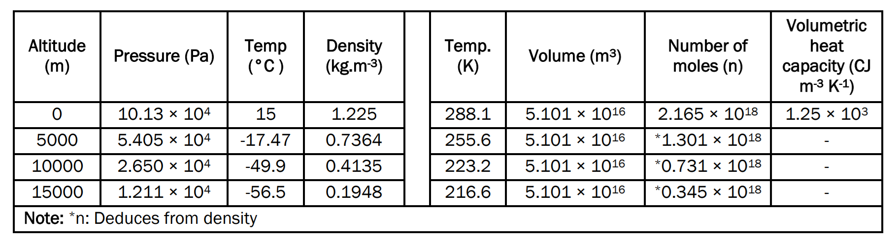
To explain this discrepancy, we examine, with the ideal gas law, to which the Earth’s atmosphere obeys with its normal conditions of pressure and temperature, the role that the adiabatic compression of the atmospheric mass subjected to gravity can play. The dimensional analysis of the ideal gas law demonstrates that compression of the atmosphere produces energy, which can be calculated in Joules.

The temperature of the atmosphere near the Earth’s surface is influenced by
its invariable atmospheric mass, solar irradiation and the greenhouse effect.

This calls into question the commonly established Earth’s energy budgets which consider almost exclusively radiative effects, and which deduce a back radiation attributed to the greenhouse effect which is abnormally high.

Earth temperature without atmosphere or greenhouse effects

Goody et al., estimated the solar energy available to heat, both directly and indirectly, the earth and its atmosphere at an average of 224 W/m-2 [1]. Applying the Stefan-Boltzmann law they assumed that the Earth radiates as a perfect black body in the infrared band at a temperature of 255.5 K (or min 17.6°C) for the effective emission temperature [2]. These authors noted that this temperature is lower than the average temperature of the Earth’s surface and indicated that much of the radiation to space must come from the atmosphere rather than from the surface. Goody et al., arbitrarily assigned a value of 1 to the emissivity ε for the calculation, while Jacquemoud assigned a value of 0.98 [3].

According to Hansen, a solar irradiance of 1367 W/m-2 or generally accepted today 1361 W/m-2, but varying with solar fluctuations, leads to a surface temperature of 255 K (or min 18°C), which induces a greenhouse effect of +33°C [4]  Cotton reported that the emission temperature is -19°C and the earth temperature is +14°C, which corresponds to a global greenhouse effect of +33°C [5]. The global greenhouse effect is also estimated at +33°C [6-8]
.
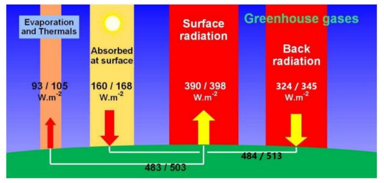
Logically, at -18°C the surface of the earth without an atmosphere or with an atmosphere totally transparent to longwave radiation and that plays no physical role, without any greenhouse effect, should be entirely frozen and covered with frost over its entire surface. This would result in a high Albedo which could be on the order of 0.5 to 0.9 instead of an albedo of 0.30 or 0.29 generally accepted in its current state. In this situation, instead of the solar energy absorbed by the surface reaching approximately 160 to 168 W/m-2 (Figure 1) this energy could be on the order of 70 W/m-2 [9-11]. The Stefan-Boltzmann formula yields a potential surface temperature of approximately -85°C [2]. Note that at these temperatures the water vapor pressure above ice is infinitesimal and could only generate an infinitesimal greenhouse effect. However, according to Nikolov et al., the effects linked to the atmosphere would bring approximately 90°C and not 33°C to the surface at a temperature of 15°C [12,13]. This would suggest that the global  natural effect of atmosphere could be on the order of 90°C rather than the 33°C of the traditional purely radiative approach as reported by almost all the authors.

Global mean energy budget of the Earth

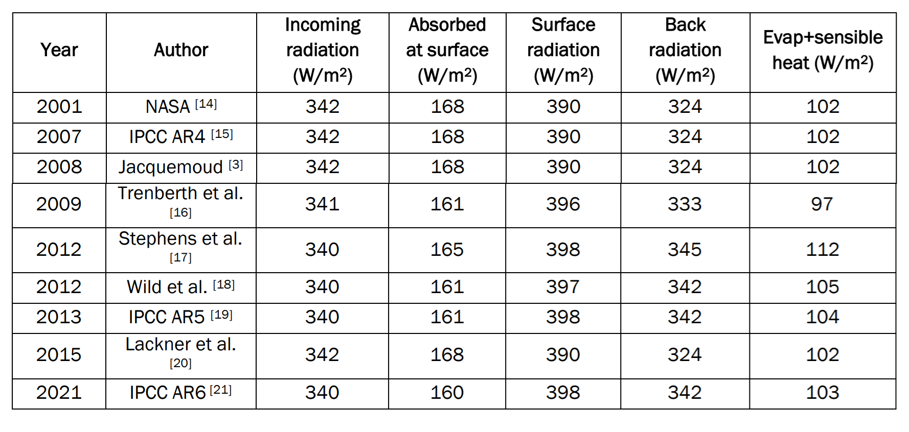
Many authors have endeavored to establish an overall assessment of the energy flows to which the earth is subjected to justify the surface temperature in an essentially radiative system. The Intergovernmental Panel on Climate Change (IPCC) itself places great emphasis on this in each of its reports. The Figure 1 summarizes the values and differences obtained while Table 1 summarizes the main authors who evaluated this earth assessment over a period of approximatively twenty years.

Figure 1. Range of nine energy balances (minimum/maximum according to the authors).

Table 1. Global energy balance of the Earth according to the authors.

The dispersion and imprecision of the results do not allow the effect on surface temperature to be deduced with sufficient accuracy. These budgets must be improved as noted by Lupo et al. [22]

Effect of atmospheric pressure

Few authors have mentioned the role that an atmospheric mass subject to gravity could play in temperature. We can nevertheless cite Leroux [23] Jelbring [24], and Chilingar [25] but these authors evoke a potential role of atmospheric pressure on a qualitative level without seeking to calculate and quantify the effects, probably given the difficulty of integrating the atmosphere as a whole. Nikolov et al. clarify the role of atmospheric pressure for several planets through a complex semiempirical iterative approach [11]

Dimensional analysis of the ideal gas law PV=nRT

The ideal gas law PV=nRT is one of the most fundamental laws of physics and applies entirely to the lower troposphere under its usual conditions of pressure and temperature. This universally accepted law, established in 1834 by Émile Clapeyron, has been perfectly stable for nearly 200 years, which is the case for very few physical laws.

  • P is the pressure (Pa);
  • V is the volume of the gas (m3);
  • n is the quantity of material (mol);
  • T is the absolute temperature (K);
  • R is the universal constant of ideal gases (8.314 J K−1 mol−1);

Dimensional analysis leads to:
R=PV/nT i.e., J K−1 mol−1=Pa.m3 K−1 mol−1, Hence J=Pa.m3=energy

The volume of air multiplied by the pressure to which it is subjected is considered energy (Joules). The atmosphere is heated by compression due to the gravitational field to which it is subjected. Isolated in space, the Earth can only exchange energy with space by radiation, but the atmospheric mass cannot radiate spontaneously since its homonuclear constituents O2, N2, and Ar are passive and cannot radiate.

The earth’s surface is warmer and the atmosphere cannot cool down on contact with it. The compression is thus adiabatic. The greenhouse gases contained in the atmosphere at low levels, mainly H2O and CO2, are capable of radiating at long wavelengths but do not interact radiatively with O2 and N2; additionally, they are under the influence of permanent terrestrial infrared radiation, which they are capable of absorbing, and which is generated continuously from the solar energy received by the Earth’s surface.

The process includes the upward expansion, toward vacuum of the agitated molecules whose kinetic energy decreases and therefore the pressure, which causes cooling with altitude. It is not due to a  decrease in gravity which decreases by less than 3/1000 at a 10 km altitude but of a struggle between gravity and the suction of the vacuum, until the equilibrium which defines an adiabatic thermal gradient. Gravity nevertheless prevents air molecules from escaping into space. Only some H2 molecules can reach the release speed.

RESULTS  Heating of the atmosphere in °K by adiabatic compression

Table 2. Data for an air layer 100 m thick. The left part is from U.S. Standard Atmosphere, according to The EngineeringToolBox [26]

As a tight approximation, for 100 m of atmospheric thickness
Altitude 0 m

  • PV=(10.13 × 10⁴ Pa) (5.101 × 10¹⁶ m3)=5.167 × 10²¹ J
  • Volumetric heat capacity of air C=1256 J m−3 K−1 (at 0 m, 15°C)
  • For 5.101 × 10¹⁶ m3 of air; +1°K requires 1256 × 5.101 × 1016 J=6.41 × 10¹⁹ J
  • 5.167 × 10²¹ J/6.41 × 1019 J=80.7
  • +80.7 K overheating due to pressure

Note: With an air layer of 200 m the precision is lower and leads to an overheating of 80.6 K

Gravity compression results, to the Earth’s surface, in 80.7°C of natural greenhouse energy equivalence, which means that to reach 15°C the initial temperature without atmosphere would be -65.7°C, very different from the -18°C admitted by radiative approaches for an inactive atmosphere.

Direct application of the ideal gas law T=PV/nR

  • Altitude 0 m T=(10.13 × 104 × 5.10 × 1016)/(2.165 × 1018 × 8.314)=287.1 K (+14.0°C)
  • Altitude 5,000 m T=254.9 K (-18.2°C)
  • Altitude 10,000 m T=222.4 K (-50.7°C)
  • Altitude 15,000 m T=215.3 K (-57.8°C)

The standard thermal gradient from 0 to 10 km is -6.49°C/km. The ideal gas law explains phenomena linked to temperatures up to 10,000 m in altitude. Beyond that, the results diverge, and other factors and phenomena are involved, like ozone and UV influence.

CONCLUSION

The temperature on the surface of the earth is mainly determined by the action of gravity on the atmospheric mass, which is an immutable fact on a scale of millennia. Climatic variations are the result of lesser phenomena. The solar influence is felt during the day by the direct radiation received, mainly when the sun is at its zenith, and the balance is modified by direct thermal exchanges between the sunny surface and the air in contact. The earth’s surface and the upper layers of the atmosphere radiate permanently towards space by emitting infrared radiation day and night, thus restoring the overall balance.

Surface infrared radiation is probably less intercepted in the lower troposphere by greenhouse molecules than is usually thought, thus explaining the surface temperature. However, there is an atmospheric dynamic, in particular through the water cycle, by evaporation-condensation, but whose overall energy balance is zero. Air mass movements and convection contribute to the overall dynamics, mainly due to the rotation of the Earth and the alternations between the presence and absence of solar radiation.

Astronomical fluctuations in sunshine, surface phenomena such as ocean currents, El Niño or La Niña phenomena, extreme weather phenomena or even volcanic eruptions, as well as other factors that are probably poorly characterized, lead to variations in surface temperature that nevertheless remain relatively damped due to the stabilizing effect of the invariable atmospheric mass subject to gravity.

See Also

Planetary Warming: Back to Basics


Again, There is No Right to a Stable Climate

Twenty-two young people from across the country sued the
Trump administration over the executive orders,
which prioritize the expansion of fossil fuels.

The complaint, filed Thursday in the U.S. District Court in Montana, challenges three executive orders: “Unleashing American Energy,” “Declaring a National Energy Emergency” and “Reinvigorating America’s Beautiful Clean Coal Industry.” The lawsuit argues that with the orders, the Trump administration knowingly is advancing an agenda that will increase greenhouse gas pollution that already is stressing the global climate to a dangerous extent.

The litigation argues the situation infringes on the young people’s constitutional rights to life and liberty, as well as falling afoul of other laws approved by Congress that protect public health and the environment. The plaintiffs want the court to declare the executive orders unconstitutional, block their implementation and reaffirm the legal limits on presidential power.

“From day one of the current administration, President Trump has issued directives to increase fossil fuel use and production and block an energy transition to wind, solar, battery storage, energy efficiency, and electric vehicles (“EVs”),” the lawsuit states. “President Trump’s EOs falsely claim an energy emergency, while the true emergency is that fossil fuel pollution is destroying the foundation of Plaintiffs’ lives.”

It’s the same argument from the same people (Our Children’s Trust) that was shot down in flames just a year ago.  There were multiple attempts to undo the damaged legal maneuver to no avail.  Below is why this latest litigation should be put out of its misery at once.

 Appeals Court Rules Against Kids’ Climate Lawsuit, May 1, 2024

Ninth Circuit Court of Appeals grants Federal government’s petition for writ of mandamus in the case of Juliana v. United States, originally filed in 2015.  Ruling excerpts are below in italics with my bolds. 20240501_docket-24-684_order

In the underlying case, twenty-one plaintiffs (the Juliana plaintiffs) claim that—by failing to adequately respond to the threat of climate change—the government has violated a putative “right to a stable climate system that can sustain human life.” Juliana v. United States, No. 6:15-CV-01517-AA, 2023 WL 9023339, at *1 (D. Or. Dec. 29, 2023). In a prior appeal, we held that the Juliana plaintiffs lack Article III standing to bring such a claim. Juliana v. United States, 947 F.3d 1159, 1175 (9th Cir. 2020). We remanded with instructions to dismiss on that basis. Id. The district court nevertheless allowed amendment, and the government again moved to dismiss. The district court denied that motion, and the government petitioned for mandamus seeking to enforce our earlier mandate. We have jurisdiction to consider the petition. See 28 U.S.C. § 1651. We grant it.

In the prior appeal, we held that declaratory relief was “not substantially likely to mitigate the plaintiffs’ asserted concrete injuries.” Juliana, 947 F.3d at 1170. To the contrary, it would do nothing “absent further court action,” which we held was unavailable. Id. We then clearly explained that Article III courts could not “step into the shoes” of the political branches to provide the relief the Juliana plaintiffs sought. Id. at 1175. Because neither the request for declaratory relief nor the request for injunctive relief was justiciable, we “remand[ed] th[e] case to the district court with instructions to dismiss for lack of Article III standing.” Id. Our mandate was to dismiss.

The district court gave two reasons for allowing amendment. First, it concluded that amendment was not expressly precluded. Second, it held that intervening authority compelled a different result. We reject each.
The first reason fails because we “remand[ed] . . . with instructions to dismiss for lack of Article III standing.” Id. Neither the mandate’s letter nor its spirit left room for amendment. See Pit River Tribe, 615 F.3d at 1079.

The second reason the district court identified was that, in its view, there was an intervening change in the law. District courts are not bound by a mandate when a subsequently decided case changes the law. In re Molasky, 843 F.3d 1179, 1184 n.5 (9th Cir. 2016). The case the court identified was Uzuegbunam v. Preczewski, which “ask[ed] whether an award of nominal damages by itself can redress a past injury.” 141 S. Ct. 792, 796 (2021). Thus, Uzuegbunam was a damages case which says nothing about the redressability of declaratory judgments. Damages are a form of retrospective relief. Buckhannon Bd. & Care Home v. W. Va. Dep’t of Health & Human Res., 532 U.S. 598, 608–09 (2001). Declaratory relief is prospective. The Juliana plaintiffs do not seek damages but seek only prospective relief. Nothing in Uzuegbunam changed the law with respect to prospective relief.

We held that the Juliana plaintiffs lack standing to bring their claims and told the district court to dismiss. Uzuegbunam did not change that. The district court is instructed to dismiss the case forthwith for lack of Article III standing, without leave to amend.

Background July 2023: Finally, a Legal Rebuttal on the Merits of Kids’ Climate Lawsuit

As reported last month, the Oregon activist judge invited the plaintiffs in Juliana vs US to reopen that case even after the Ninth Circuit shot it down.  Now we have a complete and thorough Motion from the defendant (US government) to dismiss this newest amended complaint.  Most interesting is the section under the heading starting on page 30.  Excerpts in italics with my bolds and added images.

Plaintiffs’ Claims Fail on the Merits

Because Plaintiffs’ action fails at the jurisdictional threshold, the Ninth Circuit never reached—and this Court need not reach—the merits of the claims. . . Plaintiffs’ second amended complaint, which supersedes the first amended complaint, asserts the same claims that were brought in the first amended complaint, which this Court addressed in orders that the Ninth Circuit reversed. Defendants thus renew their objection that Plaintiffs’ claims fail on the merits and should be dismissed pursuant to Fed. R. Civ. P. 12(b)(6).

A. There is no constitutional right to a stable climate system.

The Supreme Court has repeatedly instructed courts considering novel due process claims
to “‘exercise the utmost care whenever . . . asked to break new ground in this field,’… lest the liberty protected by the Due Process Clause be subtly transformed” into judicial policy preferences. More specifically, the Supreme Court has “regularly observed that the Due Process Clause specially protects those fundamental rights and liberties which are, objectively, ‘deeply rooted in this Nation’s history and tradition.’”  Plaintiffs’ request that this Court recognize an implied fundamental right to a stable climate system contradicts that directive, because such a purported right is without basis in the Nation’s history or tradition.

The proposed right to a “stable climate system” is nothing like any fundamental right ever recognized by the Supreme Court. The state of the climate is a public and generalized issue, and so interests in the climate are unlike the particularized personal liberty or personal privacy interests of individuals the Supreme Court has previously recognized as being protected by fundamental rights.  “[W]henever federal courts have faced assertions of fundamental rights to a ‘healthful environment’ or to freedom from harmful contaminants, they have invariably rejected those claims.”. Plaintiffs’ First Claim for Relief must be dismissed.

B.  Plaintiffs fail to allege a cognizable state-created danger claim.

The First Claim for Relief must also be dismissed because the Constitution does not impose an affirmative duty to protect individuals, and Plaintiffs have failed to allege a cognizable claim under the “state-created danger” exception to that rule.
As a general matter:

[The Due Process Clause] is phrased as a limitation on the State’s power to act, not as a guarantee of certain minimal levels of safety and security. It forbids the State itself to deprive individuals of life, liberty, or property without “due process of law,” but its language cannot fairly be extended to impose an affirmative obligation on the State to ensure that those interests do not come to harm through other means.

Thus, the Due Process Clause imposes no duty on the government to protect persons from harm inflicted by third parties that would violate due process if inflicted by the government.

Plaintiffs contend that the government’s “deliberate actions” and “deliberate indifference” with regard to the dangers of climate change amount to a due process violation under the state-created danger exception.

First, Plaintiffs have identified no harms to their “personal security or bodily integrity” of the kind and immediacy that qualify for the state-created danger exception. . . But here, Plaintiffs allege that general degradation of the global climate has harmed their “dignity, including their capacity to provide for their basic human needs, safely raise families, practice their religious and spiritual beliefs, [and] maintain their bodily integrity” and has prevented them from “lead[ing] lives with access to clean air, water, shelter, and food.”  Those types of harm are unlike the immediate, direct, physical, and personal harms at issue in the above-cited cases.

Second, Plaintiffs identify no specific government actions—much less government actors—that put them in such danger. Instead, Plaintiffs contend that a number of (mostly unspecified) agency actions and inactions spanning the last several decades have exposed them to harm. This allegation of slowly-recognized, long-incubating, and generalized harm by itself conclusively distinguishes their claim from all other state-created danger cases recognized by the Ninth Circuit.

Third, Plaintiffs do not allege that government actions endangered Plaintiffs in particular. . . As explained above, Plaintiffs’ asserted injuries arise from a diffuse, global phenomenon that affects every other person in their communities, in the United States, and throughout the world.

For all these reasons, there is no basis for finding a violation of Plaintiffs’ due process right under the state-created danger doctrine, and Plaintiffs’ corresponding claim must be dismissed.

C. No federal public trust doctrine creates a right to a stable climate system.

Plaintiffs’ Fourth Claim for Relief, asserting public trust claims, should be dismissed for two independent reasons. First, any public trust doctrine is a creature of state law that applies narrowly and exclusively to particular types of state-owned property not at issue here. That doctrine has no application to federal property, the use and management of which is entrusted exclusively to Congress. . .Consequently, there is no basis for Plaintiffs’ public trust claim against the federal government under federal law.

Second, the “climate system” or atmosphere is not within any conceivable federal public trust.

1. No public trust doctrine binds the federal government.

Plaintiffs rely on an asserted public trust doctrine for the proposition that the federal government must “take affirmative steps to protect” “our country’s life-sustaining climate system,” which they assert the government holds in trust for their benefit.  But because any public trust doctrine is a matter of state law only, public trust claims may not be asserted against the federal government under federal law. . . The Supreme Court has without exception treated public trust doctrine as a matter of state law with no basis in the United States Constitution.

2. Any public trust doctrine would not apply to the “climate system” or the atmosphere.

Independently, any asserted public trust doctrine does not help Plaintiffs here. Public trust cases have historically involved state ownership of specific types of natural resources, usually limited to submerged and submersible lands, tidelands, and waterways. . . The climate system or atmosphere is unlike any resource previously deemed subject to a public trust. It cannot be owned and, due to its ephemeral nature, cannot remain within the jurisdiction of any single government. No court has held that the climate system or atmosphere is protected by a public trust doctrine. Indeed, the concept has been widely rejected.

For all these reasons, the Court should dismiss Plaintiffs’ Fourth Claim for Relief.

Background Post Update on Zombie Kids Climate Lawsuits: (Juliana vs. US) (Held vs Montana)

April 2025 Two Years Ocean Warming Gone

The best context for understanding decadal temperature changes comes from the world’s sea surface temperatures (SST), for several reasons:
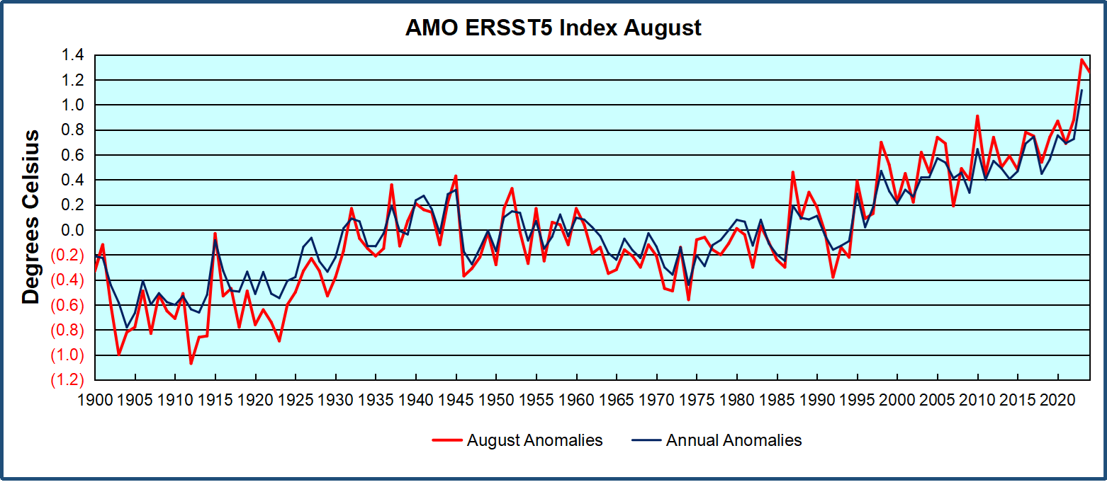
  • The ocean covers 71% of the globe and drives average temperatures;
  • SSTs have a constant water content, (unlike air temperatures), so give a better reading of heat content variations;
  • A major El Nino was the dominant climate feature in recent years.

HadSST is generally regarded as the best of the global SST data sets, and so the temperature story here comes from that source. Previously I used HadSST3 for these reports, but Hadley Centre has made HadSST4 the priority, and v.3 will no longer be updated.  HadSST4 is the same as v.3, except that the older data from ship water intake was re-estimated to be generally lower temperatures than shown in v.3.  The effect is that v.4 has lower average anomalies for the baseline period 1961-1990, thereby showing higher current anomalies than v.3. This analysis concerns more recent time periods and depends on very similar differentials as those from v.3 despite higher absolute anomaly values in v.4.  More on what distinguishes HadSST3 and 4 from other SST products at the end. The user guide for the current version HadSST4.1.1.0 is here.   The charts and analysis below is produced from the current data.

The Current Context

The chart below shows SST monthly anomalies as reported in HadSST4 starting in 2015 through April 2025. A global cooling pattern is seen clearly in the Tropics since its peak in 2016, joined by NH and SH cycling downward since 2016, followed by rising temperatures in 2023 and 2024.

Note that in 2015-2016 the Tropics and SH peaked in between two summer NH spikes.  That pattern repeated in 2019-2020 with a lesser Tropics peak and SH bump, but with higher NH spikes. By end of 2020, cooler SSTs in all regions took the Global anomaly well below the mean for this period.  A small warming was driven by NH summer peaks in 2021-22, but offset by cooling in SH and the tropics, By January 2023 the global anomaly was again below the mean.

Then in 2023-24 came an event resembling 2015-16 with a Tropical spike and two NH spikes alongside, all higher than 2015-16. There was also a coinciding rise in SH, and the Global anomaly was pulled up to 1.1°C last year, ~0.3° higher than the 2015 peak.  Then NH started down autumn 2023, followed by Tropics and SH descending 2024 to the present. After 12 months of cooling in SH and the Tropics, the Global anomaly came back down, led by NH cooling the last 8 months from its 1.3C peak in August, down to 0.8C in March and April. With some recent warming in the Tropics and SH, all regions are now close together nearly at the global anomaly, less than 0.1C higher than the average for this period.

Remarkably, April 2025 SST anomalies in all regions and globally are the coolest since March 2023.

Comment:

The climatists have seized on this unusual warming as proof their Zero Carbon agenda is needed, without addressing how impossible it would be for CO2 warming the air to raise ocean temperatures.  It is the ocean that warms the air, not the other way around.  Recently Steven Koonin had this to say about the phonomenon confirmed in the graph above:

El Nino is a phenomenon in the climate system that happens once every four or five years.  Heat builds up in the equatorial Pacific to the west of Indonesia and so on.  Then when enough of it builds up it surges across the Pacific and changes the currents and the winds.  As it surges toward South America it was discovered and named in the 19th century  It iswell understood at this point that the phenomenon has nothing to do with CO2.

Now people talk about changes in that phenomena as a result of CO2 but it’s there in the climate system already and when it happens it influences weather all over the world.   We feel it when it gets rainier in Southern California for example.  So for the last 3 years we have been in the opposite of an El Nino, a La Nina, part of the reason people think the West Coast has been in drought.

It has now shifted in the last months to an El Nino condition that warms the globe and is thought to contribute to this Spike we have seen. But there are other contributions as well.  One of the most surprising ones is that back in January of 2022 an enormous underwater volcano went off in Tonga and it put up a lot of water vapor into the upper atmosphere. It increased the upper atmosphere of water vapor by about 10 percent, and that’s a warming effect, and it may be that is contributing to why the spike is so high.

A longer view of SSTs

The graph below  is noisy, but the density is needed to see the seasonal patterns in the oceanic fluctuations.  Previous posts focused on the rise and fall of the last El Nino starting in 2015.  This post adds a longer view, encompassing the significant 1998 El Nino and since.  The color schemes are retained for Global, Tropics, NH and SH anomalies.  Despite the longer time frame, I have kept the monthly data (rather than yearly averages) because of interesting shifts between January and July.

To enlarge image, open in new tab.

The graph above is noisy, but the density is needed to see the seasonal patterns in the oceanic fluctuations.  Previous posts focused on the rise and fall of the last El Nino starting in 2015.  This post adds a longer view, encompassing the significant 1998 El Nino and since.  The color schemes are retained for Global, Tropics, NH and SH anomalies.  Despite the longer time frame, I have kept the monthly data (rather than yearly averages) because of interesting shifts between January and July. 1995 is a reasonable (ENSO neutral) starting point prior to the first El Nino.

The sharp Tropical rise peaking in 1998 is dominant in the record, starting Jan. ’97 to pull up SSTs uniformly before returning to the same level Jan. ’99. There were strong cool periods before and after the 1998 El Nino event. Then SSTs in all regions returned to the mean in 2001-2.

SSTS fluctuate around the mean until 2007, when another, smaller ENSO event occurs. There is cooling 2007-8,  a lower peak warming in 2009-10, following by cooling in 2011-12.  Again SSTs are average 2013-14.

Now a different pattern appears.  The Tropics cooled sharply to Jan 11, then rise steadily for 4 years to Jan 15, at which point the most recent major El Nino takes off.  But this time in contrast to ’97-’99, the Northern Hemisphere produces peaks every summer pulling up the Global average.  In fact, these NH peaks appear every July starting in 2003, growing stronger to produce 3 massive highs in 2014, 15 and 16.  NH July 2017 was only slightly lower, and a fifth NH peak still lower in Sept. 2018.

The highest summer NH peaks came in 2019 and 2020, only this time the Tropics and SH were offsetting rather adding to the warming. (Note: these are high anomalies on top of the highest absolute temps in the NH.)  Since 2014 SH has played a moderating role, offsetting the NH warming pulses. After September 2020 temps dropped off down until February 2021.  In 2021-22 there were again summer NH spikes, but in 2022 moderated first by cooling Tropics and SH SSTs, then in October to January 2023 by deeper cooling in NH and Tropics.

Then in 2023 the Tropics flipped from below to well above average, while NH produced a summer peak extending into September higher than any previous year.  Despite El Nino driving the Tropics January 2024 anomaly higher than 1998 and 2016 peaks, following months cooled in all regions, and the Tropics continued cooling in April, May and June along with SH dropping.  After July and August NH warming again pulled the global anomaly higher, September through January 2025 resumed cooling in all regions, continuing February through April 2025.

What to make of all this? The patterns suggest that in addition to El Ninos in the Pacific driving the Tropic SSTs, something else is going on in the NH.  The obvious culprit is the North Atlantic, since I have seen this sort of pulsing before.  After reading some papers by David Dilley, I confirmed his observation of Atlantic pulses into the Arctic every 8 to 10 years.

Contemporary AMO Observations

Through January 2023 I depended on the Kaplan AMO Index (not smoothed, not detrended) for N. Atlantic observations. But it is no longer being updated, and NOAA says they don’t know its future.  So I find that ERSSTv5 AMO dataset has current data.  It differs from Kaplan, which reported average absolute temps measured in N. Atlantic.  “ERSST5 AMO  follows Trenberth and Shea (2006) proposal to use the NA region EQ-60°N, 0°-80°W and subtract the global rise of SST 60°S-60°N to obtain a measure of the internal variability, arguing that the effect of external forcing on the North Atlantic should be similar to the effect on the other oceans.”  So the values represent SST anomaly differences between the N. Atlantic and the Global ocean.

The chart above confirms what Kaplan also showed.  As August is the hottest month for the N. Atlantic, its variability, high and low, drives the annual results for this basin.  Note also the peaks in 2010, lows after 2014, and a rise in 2021. Then in 2023 the peak was holding at 1.4C before declining.  An annual chart below is informative:


Note the difference between blue/green years, beige/brown, and purple/red years.  2010, 2021, 2022 all peaked strongly in August or September.  1998 and 2007 were mildly warm.  2016 and 2018 were matching or cooler than the global average.  2023 started out slightly warm, then rose steadily to an  extraordinary peak in July.  August to October were only slightly lower, but by December cooled by ~0.4C.

Then in 2024 the AMO anomaly started higher than any previous year, then leveled off for two months declining slightly into April.  Remarkably, May showed an upward leap putting this on a higher track than 2023, and rising slightly higher in June.  In July, August and September 2024 the anomaly declined, and despite a small rise in October, ended close to where it began.  Note 2025 started much lower than the previous year and is headed sharply downward, well below the previous two years.

The pattern suggests the ocean may be demonstrating a stairstep pattern like that we have also seen in HadCRUT4.

The purple line is the average anomaly 1980-1996 inclusive, value 0.17.  The orange line the average 1980-2024, value 0.38, also for the period 1997-2012. The red line is 2013-2024, value 0.67. As noted above, these rising stages are driven by the combined warming in the Tropics and NH, including both Pacific and Atlantic basins.

Curiosity:  Solar Coincidence?

The news about our current solar cycle 25 is that the solar activity is hitting peak numbers now and higher  than expected 1-2 years in the future.  As livescience put it:  Solar maximum could hit us harder and sooner than we thought. How dangerous will the sun’s chaotic peak be?  Some charts from spaceweatherlive look familar to these sea surface temperature charts.

Summary

The oceans are driving the warming this century.  SSTs took a step up with the 1998 El Nino and have stayed there with help from the North Atlantic, and more recently the Pacific northern “Blob.”  The ocean surfaces are releasing a lot of energy, warming the air, but eventually will have a cooling effect.  The decline after 1937 was rapid by comparison, so one wonders: How long can the oceans keep this up? And is the sun adding forcing to this process?
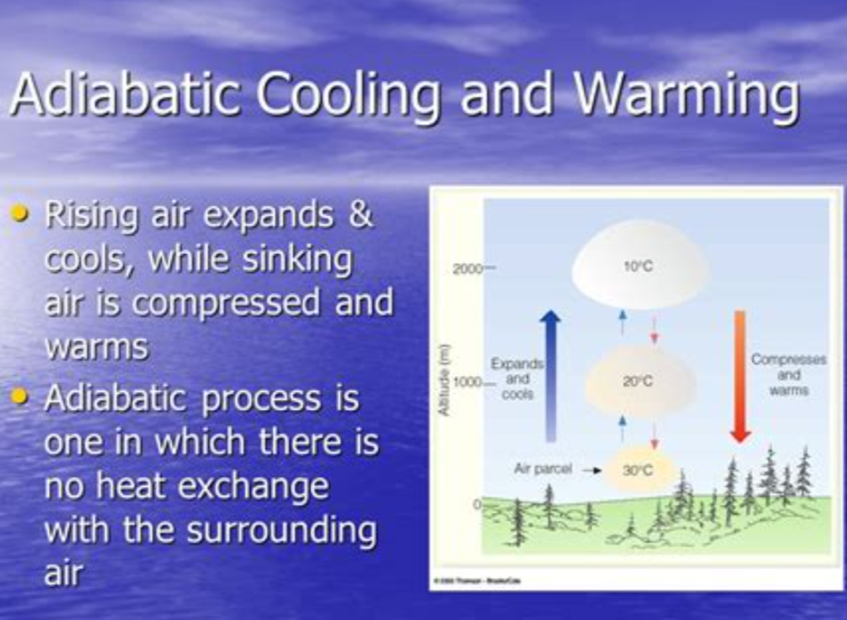
Footnote: Why Rely on HadSST4
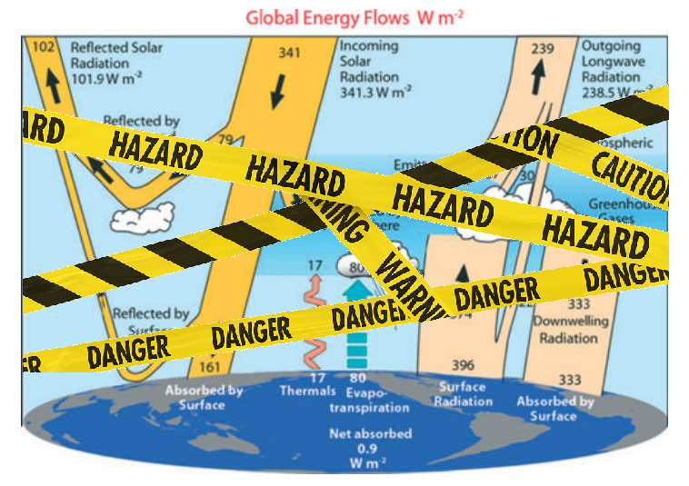
HadSST is distinguished from other SST products because HadCRU (Hadley Climatic Research Unit) does not engage in SST interpolation, i.e. infilling estimated anomalies into grid cells lacking sufficient sampling in a given month. From reading the documentation and from queries to Met Office, this is their procedure.

HadSST4 imports data from gridcells containing ocean, excluding land cells. From past records, they have calculated daily and monthly average readings for each grid cell for the period 1961 to 1990. Those temperatures form the baseline from which anomalies are calculated.

In a given month, each gridcell with sufficient sampling is averaged for the month and then the baseline value for that cell and that month is subtracted, resulting in the monthly anomaly for that cell. All cells with monthly anomalies are averaged to produce global, hemispheric and tropical anomalies for the month, based on the cells in those locations. For example, Tropics averages include ocean grid cells lying between latitudes 20N and 20S.

Gridcells lacking sufficient sampling that month are left out of the averaging, and the uncertainty from such missing data is estimated. IMO that is more reasonable than inventing data to infill. And it seems that the Global Drifter Array displayed in the top image is providing more uniform coverage of the oceans than in the past.

uss-pearl-harbor-deploys-global-drifter-buoys-in-pacific-ocean

USS Pearl Harbor deploys Global Drifter Buoys in Pacific Ocean