Update May 19, 2015 text added at end.

Earlier I wrote an essay about our living on a water world. Then an essay described the role of oceans as a climate flywheel, storing massive amounts of solar energy and thereby stabilizing fluctuations in temperature and climate. A recent post about oceans making global temperature changes drew some comments about downplaying the role of the atmosphere in climate change. So I want to clarify some things.

The Dynamic Duo

Climate change is a coupled ocean-air dynamic, stimulated by ocean heat transfers into the air, and involving the two fluids (air and water) feeding off each other.

To maintain an approximate steady state climate the ocean and atmosphere must move excess heat from the tropics to the heat deficit polar regions. Additionally the ocean and atmosphere must move freshwater to balance regions with excess dryness with those of excess rainfall. The movement of freshwater in its vapor, liquid and solid state is referred to as the hydrological cycle.

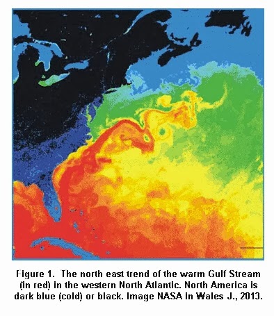
In low latitudes the ocean moves more heat poleward than does the atmosphere, but at higher latitudes the atmosphere becomes the big carrier. The wind driven ocean circulation moves heat mainly on the horizontal plane. For example, in the North Atlantic, warm surface water move northward within the Gulf Stream on the western side of the ocean, to be balanced by cold surface water moving southward within the Canary Current on the eastern side of the ocean.  The thermohaline circulation moves heat mainly in the vertical plane. For example, North Atlantic Deep Water with a temperature of about 2°C flows towards the south in the depth range 2000 to 4000 meters to be balanced by warmer water (greater than 4°C) flowing northward within the upper 1000 meters.

The ocean role in climate would be zero if there were an impervious lid over the ocean, but there is not, across the sea surface pass heat, water, momentum, gases and other materials. The wind exerts a stress on the sea surface that induces the Ekman transport and wind driven circulation.

http://eesc.columbia.edu/courses/ees/climate/lectures/o_atm.html

A lot of factors affect heat transfers from oceans to atmosphere, but the main ones are advection (heat in water flowing horizontally), mixing (vertical upwelling and downwelling of warmer and colder waters) and surface evaporation (latent heat rising with water vapor converted from liquid). The latter is greatly affected by wind which adds to the complexity of the process. For this essay, I will leave on the side the issue of sea ice dynamics, including the latent heat released in its freezing.

Ocean-atmosphere Interactions

The ocean can warm or cool the air in a number of different ways. For example, when the air is at a lower temperature than seawater, the ocean transfers heat to the lower atmosphere, which becomes less dense as the heat causes molecules in the air to move farther apart. As a result, a low-pressure air mass forms over that part of the ocean. (Conversely, cool or cold waters lead to the formation of high-pressure air masses as air molecules move closer together.) Because air always flows from areas of higher pressure to those of lower pressure, winds are diverted toward the low-pressure area.

Among winds that are affected by such pressure changes are the jet streams, bands of fast-moving, high-altitude air currents. Jet streams supply energy to developing storms at lower altitudes and then influence their movement. In this way, the ocean alters the direction of storm tracks. Some storms even reverse direction as the result of ocean-influenced air-pressure changes.

The ocean’s currents make it possible for these weather effects to be widely distributed. Some currents carry warm water from tropical and subtropical regions toward the poles, while other currents move cool water in the opposite direction. The Gulf Stream is a current that transports warm water across the North Atlantic Ocean from Florida toward Europe. Before reaching Europe, the Gulf Stream breaks up into several other currents, one of which flows to the British Isles and Norway. The heat carried in this current warms the winds that blow over these regions, helping to keep winters there from becoming bitterly cold.

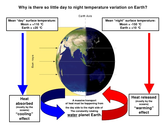
In this way, the ocean’s circulation compensates somewhat for the sun’s unequal heating of the Earth, in which the tropics receive more energy from the sun than the poles. Were it not for the moderating effects of ocean currents on air temperatures, the tropics would be much hotter than they are and the polar regions even colder.

Besides transferring heat to the atmosphere, the ocean also adds water to the air through evaporation. When the sun’s heat causes surface water to evaporate, warm water vapor rises into the atmosphere. As the water vapor rises higher, it cools into tiny water droplets and ice crystals, which collect together to form large clouds. The clouds soon return their moisture to the surface as rain, snow, sleet, or hail. Most evaporation occurs in the warm waters of the tropics and subtropics, providing moisture for tropical storms.

Virtually all rain comes from the evaporation of seawater. Though this may seem surprising, it makes sense when one considers that about 97 percent of all water on Earth is in the ocean. The Earth’s water cycle, or hydrologic cycle, consists largely of the never-ending circulation of water from the ocean to the atmosphere and then back to the ocean.

http://science.howstuffworks.com/how-the-ocean-affects-climate-info1.htm

Oceanic Oscillations

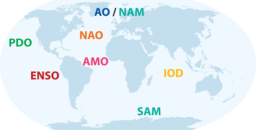
Most widely known is the El Nino Southern Oscillation, or ENSO. Many other naturally occurring ocean-atmosphere oscillations in the Pacific, Atlantic, and Indian Oceans have been recognized and named. Some of them have much more of an impact on climate and weather patterns in the U.S. and elsewhere than ENSO. As during ENSO, in many of these ocean and atmosphere interact as a coupled system, with ocean conditions influencing the atmosphere and atmospheric conditions influencing the ocean. However, not all exert as strong an influence on global weather patterns, and some are even less regular than ENSO.

Many oscillations are under study:

Antarctic Oscillation (AAO), also referred to as the Southern Annular Mode (SAM).

Arctic Oscillation (AO)

The AO and the North Atlantic Oscillation (see below) are collectively referred to as the Northern Annular Mode (NAM).

Atlantic Multidecadal Oscillation (AMO)

Indian Ocean Dipole (IOD)

Madden-Julian Oscillation (MJO)

North Atlantic Oscillation (NAO)

North Pacific Gyre Oscillation (NPGO)

North Pacific Oscillation (NPO)

Pacific Decadal Oscillation (PDO)

Pacific-North American (PNA) Pattern

http://www.whoi.edu/main/topic/el-nino-other-oscillations

Each of these patterns has its distinctive qualities, ranging from phases lasting a month or so to multi-decadal phases. Some fundamental features can be seen in all of them:

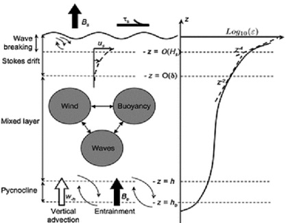
The diagram shows the vertical structure of the ocean surface boundary layer (OSBL) and the processes that deepen. The three sources of turbulence are: wind, buoyancy and waves.

The bulk of the OSBL can be termed the mixed layer, where the temperature and salinity are approximately uniform with depth, and which is often capped below, at the mixed layer depth, by a sharp pycnocline, which extends deeper into the ocean. Three sources of turbulence, namely wind, buoyancy and waves, drive turbulence in this mixed layer, which then deepens the OSBL. Hence a quantitative understanding of these turbulent processes in the OSBL is likely to be the key to understanding the shallow biases in mixed layer depth.

Deepening of the OSBL implies an increase in potential energy, and hence requires an energy source, such as turbulent kinetic energy (TKE).

Belcher, S. E., et al. (2012), A global perspective on Langmuir turbulence in the ocean surface boundary
layer, Geophys. Res. Lett., 39, L18605, doi:10.1029/2012GL052932.
http://onlinelibrary.wiley.com/doi/10.1029/2012GL052932/full

The Madden-Julian Oscillation is one of the simpler oscillations to understand, partly because of its short 30-60 day cycle.

Even so, you can see there is a lot going on, and a lot of variables affecting both strength and timing. But the same dynamic plays out in all the oscillations, including ENSO.

First, the atmosphere responds to the ocean: the atmospheric fluctuations manifested as the Southern Oscillation are mostly an atmospheric response to the changed lower boundary conditions associated with El Nino SST fluctuations.

Second, the ocean responds to the atmosphere: the oceanic fluctuations manifested as El Nino seem to be an oceanic response to the changed wind stress distribution associated with the Southern Oscillation.

Third, the El Nino-Southern Oscillation phenomenon arises spontaneously as an oscillation of the coupled ocean-atmosphere system.

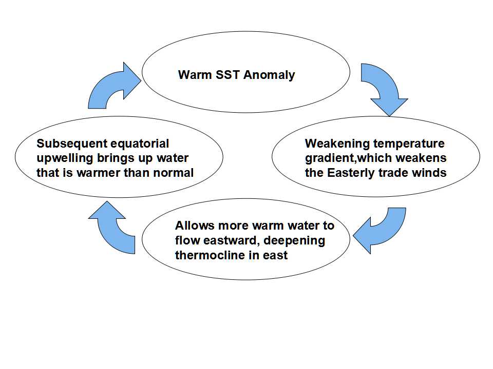
Once the El Nino event is fully developed, negative feedbacks begin to dominate the Bjerknes positive feedback, lowering the SST and bringing the event to its end after several months.

Schematic of the feedback inherent in the Pacific Ocean-atmosphere interaction. This has become known as the Bjerknes feedback.

When ocean and atmospheric conditions in one part of the world change as a result of ENSO or any other oscillation, the effects are often felt around the world. The rearrangement of atmospheric pressure, which governs wind patterns, and sea-surface temperature, which affects both atmospheric pressure and precipitation patterns, can drastically rearrange regional weather patterns, occasionally with devastating results.

Because it affects ocean circulation and weather, an El Niño or La Niña event can potentially lead to economic hardships and disaster. The potential is made worse when these combine with another, often overlooked environmental problem. For example, overfishing combined with the cessation of upwelling during an El Niño event in 1972 led to the collapse of the Peruvian anchovy fishery.

Extreme climate events are often associated with positive and negative ENSO events. Severe storms and flooding have been known to ravage areas of South America and Africa, while intense droughts and fires have occurred in Australia and Indonesia during El Niño events.

http://faculty.washington.edu/kessler/occasionally-asked-questions.html

Summary

The picture that emerges from this analysis is that the wind-driven meridional overturning circulation in the upper Pacific Ocean has been slowing down since the 1970s. This slowdown can account for the recent anomalous surface warming in the tropical Pacific, as the supply of cold pycnocline water originating at higher latitudes to feed equatorial upwelling has decreased. The Southern Hemisphere is responsible for about half of the observed decrease in equatorward pycnocline transport. Thus, perspectives on decadal variability limited to the Northern Hemisphere alone are incomplete. The fact that few studies have considered a role for the Southern Hemisphere ocean is presumably a consequence of limited data availability rather than a lack of decadal signal in the southern tropics and Subtropics.

The oceanic and atmospheric processes that we have described work together so as to reinforce each other, similar to the positive feedbacks that occur during ENSO events. For example, weaker easterly trade winds in the equatorial Pacific would result in reduced Ekman and geostrophic meridional transports, reduced equatorial upwelling, and warmer equatorial sea surface temperatures. Warmer surface temperatures in turn would alter patterns of deep atmospheric convection so as to favour weaker trade winds. If the system is to oscillate on decadal timescales, then delayed negative feedback mechanisms, one candidate for which involves planetary scale ocean waves, must also be important.

Similarities in the spatial structures of the PDO and ENSO (both, for example, have phases that are characterized by warm tropics and a cool central North Pacific, and vice versa) have raised questions about the possible interaction between interannual- and decadal timescale phenomena in the Pacific. In particular, since 1976±77 there have been fewer La Nina events, and more frequent, stronger, and longer-lasting El Nino events.

Whether this recent change in the character of the ENSO cycle is a consequence or a cause of underlying decadal-timescale variability is unknown. It could be that the decadal changes in circulation described here operate independently from those that affect the ENSO cycle. If so, they would modify the background state on which ENSO develops, and thereby precondition interannual fluctuations to preferred modes of
behaviour. Alternatively, the observed decadal changes may simply be the low-frequency residual of random or chaotic fluctuations in tropical ocean±atmosphere interactions that give rise to the ENSO cycle itself. In either case, a complete understanding of climate variability spanning interannual to decadal timescales in the Pacific basin will need to account for the slowly varying meridional overturning circulation between the tropics and subtropics.

Click to access mcphaden+zhang_nature_2002.pdf

Conclusion

Ocean oscillations are profoundly uncertain, not only because each one is erratic in the timing and strength of phase changes, but also because they have interactive effects upon each other. And with time cycles differing from 1-2 months to 30-60 years the complexity of movements is enormous.

Even today, after many years of study by highly intelligent people, the factors are murky enough that coupled ocean-atmospheric models still lack skill to forecast the patterns. And so, in 2015, we find advocates for reducing use of fossil fuels hoping and praying for a warm water blob in the Northern Pacific to intensify or endure so that the average global temperature will trend higher than last year.

Of course, the satellite records have 1998 as the warmest year by a wide margin. And why was that year so warm? It was a super El Nino. This is Oceans making climate, no mistake about it.

Update May 19, 2015

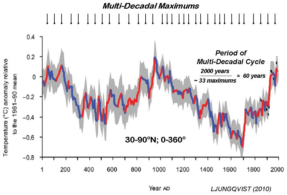
Dr. William Gray adds the longer term context to these oscillations in his 2012 paper:

“The global surface warming of about 0.7°C that has been experienced over the last 150 years and the multi-decadal up-and-down global temperature changes of 0.3-0.4°C that have been observed over this period are hypothesized to be driven by a combination of multi-century and multi-decadal ocean circulation changes. These ocean changes are due to naturally occurring upper ocean salinity variations. Changes in CO2 play little role in these salinity driven ocean climate forcings. “

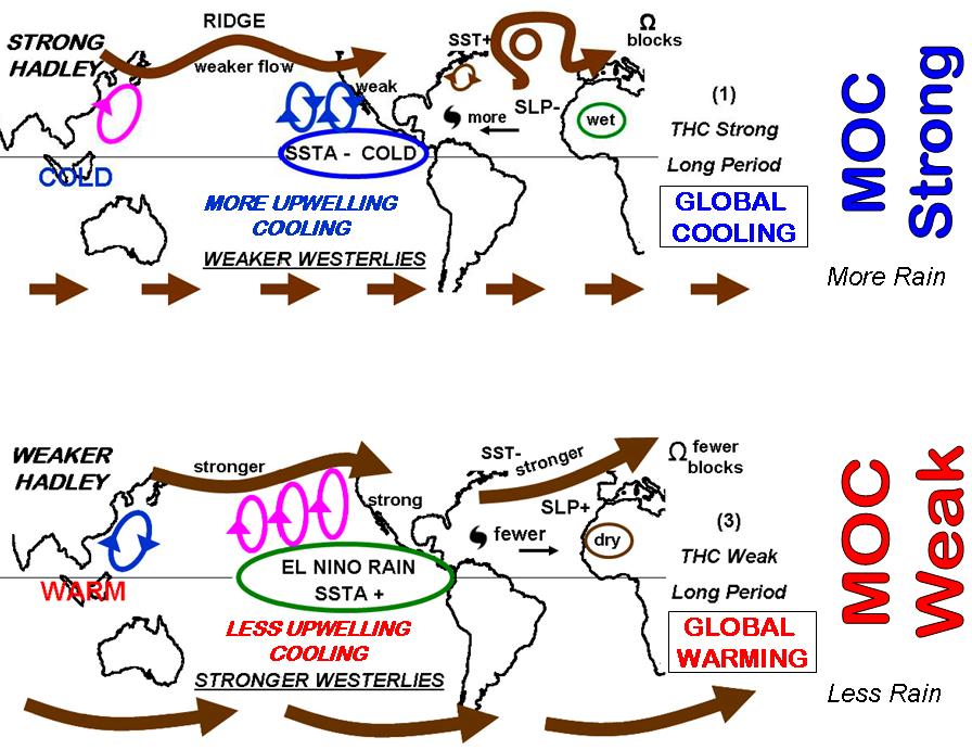
Many ocean-climate dynamics are explained in Dr. Gray’s paper:

http://tropical.atmos.colostate.edu/Includes/Documents/Publications/gray2012.pdf

Included are excellent diagrams and charts, such as these:

The Dynamic Duo: Ocean and Air

Oceans make climate is by partnering with the atmosphere. It’s a match made in heaven: Ocean is dense, powerful, slow and constrained; Atmosphere is thin, light, fast and free. Ocean has solar heat locked in its Abyss, Atmosphere is open to the cold of space. Together they take on the mission of spreading energy far and wide from the equator to the poles, and into space, the final frontier.

Here’s how it goes. Working together as companion fluids, and feeding off each other, they make winds, waves, weather and climate.

But make no mistake: Ocean is Batman, Atmosphere is Robin; Ocean is Captain Kirk, Atmosphere is Spock; Ocean the dog, Atmosphere the tail.

As for the villainous CO2, that does not rise to the level of Joker or Penguin; CO2 is probably best cast as the Riddler:

Updated May 11,18 and 19 with text added at the end.

Further update on May 27 at the end.

You only have to compare Sea Surface Temperatures (SST) from HADSST3 with estimates of Global Mean Surface Temperatures (GMST) from Hadcrut4 and RSS.

This first graph shows how global SST has varied since 1850. There are obvious changepoints where the warming or cooling periods have occurred.

This graph shows in green Hadcrut4 estimates of global surface temperature, including ocean SST, and near surface air temperatures over land. The blue line from RSS tracks lower tropospheric air temperatures measured by satellites, not near the surface but many meters higher. Finally, the red line is again Hadsst3 global SST All lines use 30-month averages to reduce annual noise and display longer term patterns.

Strikingly, SST and GMST are almost synonymous from the beginning until about 1980. Then GMST diverges with more warming than global SST. Satellite TLT shows the same patterns but with less warming than the surface. Curious as to the post 1980s patterns, I looked into HADSST3 and found NH SST warmed much more strongly during that period.

This graph shows how warming from circulations in the Northern Pacific and Northern Atlantic drove GMST since 1980. And it suggests that since 2005 NH SST is no longer increasing, and may turn toward cooling.

Surface Heat Flux from Ocean to Air

Now one can read convoluted explanations about how rising CO2 in the atmosphere can cause land surface heating which is then transported over the ocean and causes higher SST. But the interface between ocean and air is well described and measured. Not surprisingly it is the warmer ocean water sending heat into the atmosphere, and not the other way around.

The graph displays measures of heat flux in the sub-tropics during a 21-day period in November. Shortwave solar energy shown above in green labeled radiative is stored in the upper 200 meters of the ocean. The upper panel shows the rise in SST (Sea Surface Temperature) due to net incoming energy. The yellow shows latent heat cooling the ocean, (lowering SST) and transferring heat upward, driving convection.

From
An Investigation of Turbulent Heat Exchange in the Subtropics
James B. Edson

“One can think of the ocean as a capacitor for the MJO (Madden-Julian Oscillation), where the energy is being accumulated when there is a net heat flux into the ocean (here occurring to approximately November 24) after which it is released to the atmosphere during the active phase of the MJO under high winds and large latent heat exchange.”

Click to access mmedson.pdf

Conclusion

As we see in the graphs ocean circulations change sea surface temperatures which then cause global land and sea temperatures to change. Thus, oceans make climate by making temperature changes.

On another post I describe how oceans also drive precipitation, the other main determinant of climate. Oceans make rain, and the processes for distributing rain over land are shown here: https://rclutz.wordpress.com/2015/04/30/here-comes-the-rain-again/

And a word from Dr. William Gray:

“Changes in the ocean’s deep circulation currents appears to be, by far, the best physical explanation for the observed global surface temperature changes (see Gray 2009, 2011, 2012, 2012). It seems ridiculous to me for both the AGW advocates and us skeptics to so closely monitor current weather and short-time climate change as indication of CO2’s influence on our climate. This assumes that the much more dominant natural climate changes that have always occurred are no longer in operation or have relevance.”

http://www.icecap.us/

Indeed, Oceans Make Climate, or as Dr. Arnd Bernaerts put it:
“Climate is the continuation of oceans by other means.”

Update 1 May 11, 2015

Kenneth Richards provided some supporting references in a comment at Paul Homewood’s site. They are certainly on point especially this one:
“Examining data sets of surface heat flux during the last few decades for the same region, we find that the SST warming was not a consequence of atmospheric heat flux forcing. Conversely, we suggest that long-term SST warming drives changes in atmosphere parameters at the sea surface, most notably an increase in latent heat flux, and that an acceleration of the hydrological cycle induces a strengthening of the trade winds and an acceleration of the Hadley circulation.”

That quote is from Servain et al, unfortunately behind a paywall.  The paper is discussed here:

http://hockeyschtick.blogspot.ca/2014/09/new-paper-finds-climate-of-tropical.html

Full comment from Richards:

http://journals.ametsoc.org/doi/abs/10.1175/JCLI-D-13-00651.1
The surface of the world’s oceans has been warming since the beginning of industrialization. In addition to this, multidecadal sea surface temperature (SST) variations of internal [natural] origin exist. Evidence suggests that the North Atlantic Ocean exhibits the strongest multidecadal SST variations and that these variations are connected to the overturning circulation. This work investigates the extent to which these internal multidecadal variations have contributed to enhancing or diminishing the trend induced by the external radiative forcing, globally and in the North Atlantic. A model study is carried out wherein the analyses of a long control simulation with constant radiative forcing at preindustrial level and of an ensemble of simulations with historical forcing from 1850 until 2005 are combined. First, it is noted that global SST trends calculated from the different historical simulations are similar, while there is a large disagreement between the North Atlantic SST trends. Then the control simulation is analyzed, where a relationship between SST anomalies and anomalies in the Atlantic meridional overturning circulation (AMOC) for multidecadal and longer time scales is identified. This relationship enables the extraction of the AMOC-related SST variability from each individual member of the ensemble of historical simulations and then the calculation of the SST trends with the AMOC-related variability excluded. For the global SST trends this causes only a little difference while SST trends with AMOC-related variability excluded for the North Atlantic show closer agreement than with the AMOC-related variability included. From this it is concluded that AMOC [Atlantic meridional overturning circulation] variability has contributed significantly to North Atlantic SST trends since the mid nineteenth century.
—–
http://link.springer.com/article/10.1007%2Fs00382-014-2168-7
After a decrease of SST by about 1 °C during 1964–1975, most apparent in the northern tropical region, the entire tropical basin warmed up. That warming was the most substantial (>1 °C) in the eastern tropical ocean and in the longitudinal band of the intertropical convergence zone. Examining data sets of surface heat flux during the last few decades for the same region, we find that the SST [sea surface temperature] warming was not a consequence of atmospheric heat flux forcing [greenhouse gases]. Conversely, we suggest that long-term SST warming drives changes in atmosphere parameters at the sea surface, most notably an increase in latent heat flux, and that an acceleration of the hydrological cycle induces a strengthening of the trade winds and an acceleration of the Hadley circulation. These trends are also accompanied by rising sea levels and upper ocean heat content over similar multi-decadal time scales in the tropical Atlantic. Though more work is needed to fully understand these long term trends, especially what happens from the mid-1970’s, it is likely that changes in ocean circulation involving some combination of the Atlantic meridional overtuning circulation [AMOC] and the subtropical cells are required to explain the observations.
—–
http://www.nature.com/ncomms/2014/141208/ncomms6752/full/ncomms6752.html
The Atlantic Meridional Overturning Circulation (AMOC) is a key component of the global climate system, responsible for a large fraction of the 1.3 PW northward heat transport in the Atlantic basin. Numerical modelling experiments suggest that without a vigorous AMOC, surface air temperature in the North Atlantic region would cool by around 1–3 °C, with enhanced local cooling of up to 8 °C in regions with large sea-ice changes. Substantial weakening of the AMOC would also cause a southward shift of the inter-tropical convergence zone, encouraging Sahelian drought, and dynamic changes in sea level of up to 80 cm along the coasts of North America and Europe.

Update 2 May 18, 2015

This graph from Mike at climategrog shows more empirical evidence for ocean climate making, this time the relation to CO2 concentrations. The chart shows a high correlation between rates of change, not comparing directly the temperature or CO2 values or anomalies. Thus, a positive datapoint in the graph means an increase in the rate of change, negative being the rate changing downward.

The correlation is clear. There is no credible case for claiming that changes in CO2 cause changes in SST. Plenty of evidence that SST is the cause and CO2 the effect.

Update 3 May 19, 2015

On the ocean-air heat flux

Summary from
http://eesc.columbia.edu/courses/ees/climate/lectures/o_atm.html

Much of the direct and diffuse solar short wave (less than 2 micros, mostly in the visible range) electromagnetic radiation that reaches the sea surface penetrates the ocean heating the sea water down to about 100 to 200 meters. Solar heating of the ocean on a global average is 168 watts per square meter

The infrared radiation emitted from the ocean is quickly absorbed and re-emitted by water vapor and carbon dioxide and other greenhouse gases residing in the lower atmosphere. Much of the radiation from the atmospheric gases, also in the infrared range, is transmitted back to the ocean, reducing the net long wave radiation heat loss of the ocean. Net back radiation cools the ocean, on a global average by 66 watts per square meter.

When air is contact with the ocean is at a different temperature than that the sea surface, heat transfer by conduction takes place. On average the ocean is about 1 or 2 degrees warmer than the atmosphere so on average ocean heat is transferred from ocean to atmosphere by conduction.

If the ocean were colder than the atmosphere (which of course happens) the air in contact with the ocean cools, becoming denser and hence more stable, more stratified. As such the conduction process does a poor job of carrying the atmosphere heat into the cool ocean. On global average the oceanic heat loss by conduction is only 24 watts per square meter.

The largest heat loss for the ocean is due to evaporation, which links heat exchange with hydrological cycle (Fig. 4). On global average the heat loss by evaporation is 78 watts per square meter.

Update 4 May 19, 2015

Dr. William Gray in his 2012 paper:

“The global surface warming of about 0.7°C that has been experienced over the last 150 years and the multi-decadal up-and-down global temperature changes of 0.3-0.4°C that have been observed over this period are hypothesized to be driven by a combination of multi-century and multi-decadal ocean circulation changes. These ocean changes are due to naturally occurring upper ocean salinity variations. Changes in CO2 play little role in these salinity driven ocean climate forcings. “

Click to access gray2012.pdf

Update 5 May 27, 2015

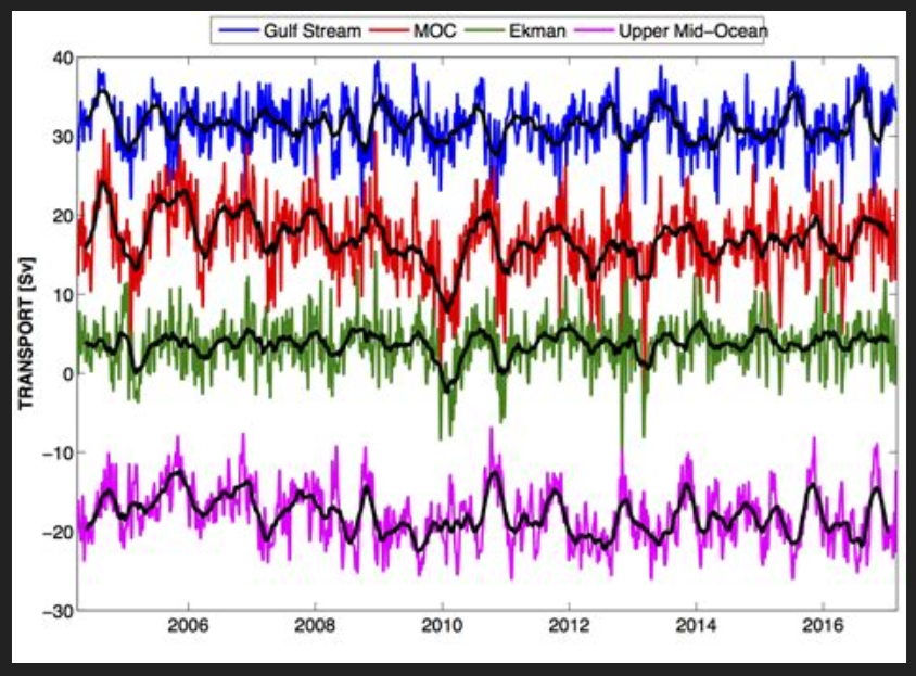
The RAPID moorings being deployed. Credit: National Oceanography Centre

A new study, by scientists from the University of Southampton and National Oceanography Centre (NOC), implies that the global climate is on the verge of broad-scale change that could last for a number of decades. This new climatic phase could be half a degree cooler.

The change to the new set of climatic conditions is associated with a cooling of the Atlantic, and is likely to bring drier summers in Britain and Ireland, accelerated sea-level rise along the northeast coast of the United States, and drought in the developing countries of the Sahel region. Since this new climatic phase could be half a degree cooler, it may well offer a brief reprise from the rise of global temperatures, as well as resulting in fewer hurricanes hitting the United States.

The study, published in Nature, proves that ocean circulation is the link between weather and decadal scale climatic change. It is based on observational evidence of the link between ocean circulation and the decadal variability of sea surface temperatures in the Atlantic Ocean.

Lead author Dr Gerard McCarthy, from the NOC, said: “Sea-surface temperatures in the Atlantic vary between warm and cold over time-scales of many decades. These variations have been shown to influence temperature, rainfall, drought and even the frequency of hurricanes in many regions of the world. This decadal variability, called the Atlantic Multi-decadal Oscillation (AMO), is a notable feature of the Atlantic Ocean and the climate of the regions it influences.”

The strength of ocean currents has been measured by a network of sensors, called the RAPID array, which have been collecting data on the flow rate of the Atlantic meridonal overturning circulation (AMOC) for a decade.

Dr David Smeed, from the NOC and lead scientist of the RAPID project, adds: “The observations of AMOC from the RAPID array, over the past ten years, show that it is declining. As a result, we expect the AMO is moving to a negative phase, which will result in cooler surface waters. This is consistent with observations of temperature in the North Atlantic.”

http://www.sciencedaily.com/releases/2015/05/150527133932.htm

And an observation from Dr. Robert E. Stevenson:

“The atmosphere cannot warm until the underlying surface warms first. The lower atmosphere is transparent to direct solar radiation, preventing it from being significantly warmed by sunlight alone. The surface atmosphere thus gets its warmth in three ways: from direct contact with the oceans; from infrared radiation off the ocean surface; and, from the removal of latent heat from the ocean by evaporation. Consequently, the temperature of the lower atmosphere is largely determined by the temperature of the ocean.”

http://www.21stcenturysciencetech.com/articles/ocean.html

 

Updates 1 and 2 at bottom.

I recently came across this comment:

“During the height of the day at the equator, 1361 joules/m2/second (less 30% Albedo) is coming in from the Sun but the surface temperature only increases as if 0.0017 joules/m2/second is absorbed (or impacts the temperature at 2 meters). The extra 959.9983 joules/m2/second flows away from the surface effectively almost as fast as the energy is coming in.

Your calculator says surface temperatures should increase to 87C.

At night, virtually no radiation is coming in (and the upwelling less downwelling radiation) says the surface should be losing about 100 joules/m2/second but it actually only loses 0.001 joules/m2/second.

This is the real-world now versus the theoretical.” Bill Illis

http://wattsupwiththat.com/2011/02/13/a-conversation-with-an-infrared-radiation-expert/

And then Derek John posted this:

I was intrigued by the wheel in the diagram, but also puzzled about the numbers. In comparison to the moon, the earth’s temperature decrease is small, but still the image shows overnight cooling on average from 20C to 10C, in contradiction to the Illis comment above.

Digging deeper, I read in Wikipedia that diurnal SST (Sea Surface Temperature) is measured to vary on calm days by about 6C. But what it said next opened my eyes: “The temperature of the ocean at depth lags the Earth’s atmosphere temperature by 15 days per 10 meters (33 ft), which means for locations like the Aral sea, temperatures near its bottom reach a maximum in December and a minimum in May and June.”

You see? Illis is talking about the accumulation of heat, and the diagram shows surface temperatures, “surface” being the key word. In infrared remote sensing methodology the radiation emanates from the top “skin” of the ocean, approximately the top 0.01 mm or less. A 6C change there is nothing compared to the massive thermal capacity underneath.  After all, the top 2 meters of the ocean match the entire heat in the overlaying atmosphere. And land surface temperatures aren’t measuring the surface, but rather the air 1 meter up. Sure the soil cools off at night, but go down even a few centimeters, and the warmth remains. People would not have built and lived in underground villages in places like Cappadocia if the land gave up its heat so readily.

And so I can understand something else Bill Illis said:

“The energy represented by a solar photon spends an average 43 hours in the Earth system before it is lost to space. Some spend just a millisecond while a very, very tiny percentage might get absorbed in the deep ocean and spend a thousand years on Earth or longer. In essence, the Earth has accumulated 1.9 days worth of solar energy. If the Sun did not come up tomorrow, it would take around 86 hours for at least the land temperature to fall below -200C.”
http://wattsupwiththat.com/2011/02/13/a-conversation-with-an-infrared-radiation-expert/#more-33954

6m (20ft) flywheel, weighs 15 tonnes. Used at Gepps Cross, Adelaide, South Australia Meatworks

The Oceans function as a Thermal Energy Flywheel

I’m speaking metaphorically, since flywheels like the one pictured above store rotational energy, and thereby maintain a steady rate, resisting periodic fluctuations. It seems that oceans have the same effect on the climate, by storing thermal energy from the sun. That’s where most of the 1.9 days of solar energy is circulating. The general term would be “accumulator”, such as rechargeable batteries, capacitors, or hydroelectric reservoirs. But I want to use flywheel because it is always in motion like the seas. And there is a precedent:

“The ocean is truly the flywheel of the climate system. By definition, a flywheel gains its efficiency from interactions with other parts of the system. Climate is determined, to a large extent, by the rates of energy transfer across the sea surface. It is these rates that determine the lag times and feedback loops and so ultimately the character of climate fluctuations in the oceans and elsewhere.”

Eric B. Kraus, 1987, ‘Oceans, Climate of’, in: Rhodes W. Fairbridge (ed.), The Encyclopaedia of Climatology (Earth Science), 1987, p.638-642

Models Missing the Ocean Flywheel

Climate science has been obsessed with only a part of the system, namely the atmosphere and radiation, in order to focus attention on the non-condensing IR active gases. The climate is framed as a 3D atmosphere above a 2D surface. That narrow scope leaves out the powerful non-radiative heat transfer mechanisms that dominate the lower troposphere, and the vast reservoir of thermal energy deep in the oceans.

As Dr. Robert E Stevenson writes, it could have been different:

“As an oceanographer, I’d been around the world, once or twice, and I was rather convinced that I knew the factors that influenced the Earth’s climate. The oceans, by virtue of their enormous density and heat-storage capacity, are the dominant influence on our climate. It is the heat budget and the energy that flows into and out of the oceans that basically determines the mean temperature of the global atmosphere. These interactions, plus evaporation, are quite capable of canceling the slight effect of man-produced CO2.”

In 1991, when the IUGG and its associations met in Vienna for their General Assembly, the presidents and the secretaries-general of the four associations I’ve mentioned, discussed the program we would propose to forward to the International Commission of Scientific Unions (ICSU) for consideration at the 1992 Rio de Janeiro Conference. We all decided not to prepare any programs!

In our joint statement, which I paraphrase here, we noted that “To single out one variable, namely radiation through the atmosphere and the associated ‘greenhouse effect,’ as being the primary driving force of atmospheric and oceanic climate, is a simplistic and absurd way to view the complex interaction of forces between the land, ocean, atmosphere, and outer space.”

Furthermore, we stated, “climate modeling has been concentrated on the atmosphere with only a primitive representation of the ocean.” Actually, some of the early models depict the oceans as nearly stagnant. The logical approach would have been to model the oceans first (there were some reasonable ocean models at the time), then adding the atmospheric factors.

Well, no one in ICSU nor the United Nations Environment Program/World Meteorological Organization was ecstatic about our suggestion. Rather, they simply proceeded to evolve climate models from early weather models. That has imposed an entirely atmospheric perspective on processes which are actually heavily dominated by the ocean.”

http://www.21stcenturysciencetech.com/articles/ocean.html

Efforts to Model the Ocean Flywheel

In the real world, radiative heat loss is determined by the temperature differential, fixed at the top of the atmosphere by the vacuum of space, and maintained at the bottom of the atmosphere by the oceans. The surface temperatures are noisy because the water is always in motion, made chaotic by flowing over and around irregular land masses. But the oceans’ bulk keeps the temperature within a remarkably tight range over the millennia.

More recently, the computer-driven models are coupled with ocean models, but often these are appendages, added on trying to improve the performance of atmospheric circulation. One of the features of these models is the setting used for the oceans’ “inertia”, which affects how slowly the artificial system responds to changes. The flywheel is a better metaphor since the oceans are always in motion while stabilizing temperatures and climate.

 

Some models are starting to have dynamic linking of ocean heat storage and circulation to the atmosphere. Results are proving interesting:

Climate Sensitivity to Changes in Ocean Heat Transport
Marcelo Barreiro et al 2011
http://journals.ametsoc.org/doi/full/10.1175/JCLI-D-10-05029.1

“According to our model, if the OHT increases further from present-day values, it would cool the global climate. Moreover, it shows large sensitivity to relatively small changes: a 25% increase in OHT cools the climate by more than 4 K (Fig. 2a). Further increases (beyond 25%) would also cool the climate but more gradually. The transition from a warming to a cooling effect of increased OHT is not gradual but abrupt. To better resolve this transition, we ran additional experiments for c = 1.05, 1.1, 1.15, and 1.20. Our results show that the occurrence of a warmer climate with increased OHT is valid for c < 1.15, which is for less than a 15% increase in the present-day values. Thus, in this model, the current climate is such that the ocean heat transport is close to its maximum positive influence.”

“To date, our understanding of the climatic response to changed OHT comes mainly from atmospheric models coupled to fixed oceans (e.g., W03, H05). Our results point out that not only is the lack of dynamical adjustment an important issue when using these models, but also that the parameterization of low clouds can result in cloud–SST radiative feedbacks of different strengths. In the end, only through the use of coupled models that allow the interaction between these processes will it be possible to address this question fully. Nonetheless, we believe the results presented here can serve as a guide for future explorations of the role of the oceans in climate.”

Another Gift from the Seas

It turns out that not only do the oceans maintain the mild habitat to which we are adapted, they also leave a climate record on the ocean floor. On longer time scales, the ocean flywheel is overwhelmed by orbital changes to the incoming solar energy, triggering regime shifts between the “Hot House” and the “Ice House”. Between shifts, the flywheel maintains the new steady state.

“There are also d18O isotopes which have proven to be very reliable proxies for temperature in the distant past. There are even International Standards for how to use these proxies to estimate temperature. Search Vienna Standard Mean Ocean Water if you want to know more about this.

The climate history charts in the article at the main post are based on this proxy of course.

There are d18O isotopes which have been dated going back all the way to 2.6 billion years ago. In total, there are 40,000 dated dO18 proxies covering the periods back to this time. 40,000 reliable proxies is more than enough to make a call about this history.

Here are the temperature estimates and all of the CO2 estimates over the last 40 million years (the data used in the paper are in this chart but I am using all the reliable numbers that there are, so rather than 8 data points, there is a total of 16,000 datapoints here between temps and CO2).”

When one runs the numbers in the proper way with these isotopes, one gets very close to Scotese’s temperature history. They can produce a higher resolution history than Scotese, however, which matches to a “T” the major developments in climate history that we know about from other disciplines like geology, paleontology etc.”  Bill Illis

http://wattsupwiththat.com/2015/04/15/strong-evidence-for-rapid-climate-change-found-in-past-millenia/#comment-1908208

Summary

Dr. Stevenson summarizes:

“Contrary to recent press reports that the oceans hold the still-undetected global atmospheric warming predicted by climate models, ocean warming occurs in 100-year cycles, independent of both radiative and human influences.”

“Inland locations are less restrained by the oceans, so the surface air experiences a wider temperature range than it does over the oceans. Land cannot store heat for long, which is why hot days are quickly followed by cold nights in desert regions. For most of the Earth, however, the more dominant ocean temperatures fix the air temperature.”

“This happens through several means:

(1) The oceans transport heat around the globe via massive currents which sweep grandly through the various ocean basins. As a result, the tropics are cooler than they would be otherwise, and the lands of the high latitudes are warmer. The global circulation of heat in the oceans moderates the air temperatures around the whole world.

(2) Because of the high density/specific heat of sea water, the entire heat in the overlying atmosphere can be contained in the top two meters of the oceans. This enormous storage capacity enables the oceans to “buffer” any major deviations in temperature, moderating both heat and cold waves alike.

(3)Evaporation is constantly taking place at the surface of the seas. It is greatest in the tropics and weakest near the polar regions. The effect of evaporation is to cool the oceans and, thereby, the surface atmosphere.”
http://www.21stcenturysciencetech.com/articles/ocean.html

Conclusion

In the real world climate, water in all its phases is the heart of the matter, and atmosphere is ancillary. Since Copernicus we all think of our planetary system with the sun in the center. We should be thinking of our climate system with the oceans in the center.

How inappropriate to call this planet Earth when it is quite clearly Ocean. Arthur C. Clarke

I have been trying to make sense of these things, and this post is the result. Thank you to Bill Illis, Robert Stevenson and Arnd Bernaerts for writings I just discovered and which crystallized my thinking. Ron Clutz

Update 1 April 24: Discussion with David A. Is elevated to a post here:
https://rclutz.wordpress.com/2015/04/24/on-the-energy-highway-with-david-a-all-watts-are-not-created-equal/

Update 2 April 25: This essay mentions d18O from ocean sediments as a proxy for climate change. Below is linked an interesting study using these to reconstruct Norwegian Sea SST over several centuries

Comment by kennethrichards at Paul Homewood website:

And the warmer oceans during the MWP and modern times are explained (> 99% significance) by the solar variations at these times…the “medieval and modern [solar] maxima.”
—–
http://onlinelibrary.wiley.com/doi/10.1029/2010JC006264/full

“Here we present an exceptionally well-dated marine sediment sequence in the eastern Norwegian Sea which records 1–2°C variations of temperature in northward flowing Atlantic waters that are robustly correlated with various estimates of solar activity spanning the last 1000 years. The temperature and solar proxy variations appear to be synchronous within dating errors, which, together with the large amplitude of the temperature signal and its correlation into central Europe, suggests strong coupling of the regional atmospheric and oceanic responses to the Sun.”

Solar forcing of ocean SST . . .Hummmm.  The plot thickens.

 

Update May 19, 2015 text added at end.

We hear a lot about CO2 as climate’s “control knob, but about the oceans’ pacemaker, AMOC? Not so much.

In the Water World post, I referenced the match between SSTs (sea surface temperatures) as recorded in HadISSAT and the IPO, an index of SSTs in the Eastern Pacific: North, Central and South. This is a brief discussion of the Atlantic role in shaping climate patterns, especially in Europe and North America.

The Big Picture

Since global average temperatures are dominated by the oceans as measured by SSTs, it is significant that multidecadal cycles are presently shifting from warmer phases to cooler. The PDO entered its cooler period recently, and the current weak El Nino is evidence of this. (Pacific Decadal Oscillation is an index of Northeastern Pacific based upon ~30-year periods, warm when El Ninos dominate, and cool when La Ninas rule.)

Atlantic Multidecadal Oscillation (AMO). Source: http://www.appinsys.com/globalwarming/SixtyYearCycle.htm

Now the focus is on the Atlantic SSTs and what to expect from the AMO (Atlantic Multidecadal Oscillation), which has peaked and is likely to trend downward. In the background is a large scale actor, the Atlantic Meridional Overturning Circulation (AMOC) which is the Atlantic part of the global “conveyor belt” moving warm water from the equatorial oceans to the poles and back again.

The notion of the AMOC as the climate pacemaker derives from its role in conveying Pacific shifts into the Atlantic.

“An index of AMOC variability is defined, and the manner in which key variables covary with it is determined. In both models the following is found. (i) AMOC variability is associated with upper-ocean (top 1 km) density anomalies (dominated by temperature) on the western margin of the basin in the region of the Mann eddy with a period of about 20 years. These anomalies modulate the trajectory and strength of the North Atlantic Current. The importance of the western margin is a direct consequence of the thermal wind relation and is independent of the mechanisms that create those density anomalies. (ii) Density anomalies in this key region are part of a larger-scale pattern that propagates around the subpolar gyre and acts as a “pacemaker” of AMOC variability. (iii) The observed variability is consistent with the primary driving mechanism being stochastic wind curl forcing, with Labrador Sea convection playing a secondary role.”

http://journals.ametsoc.org/doi/full/10.1175/JCLI-D-11-00460.1

The Atlantic Leading the Stadium Wave

The critical role of the AMOC and the Atlantic’s global influence is described as part of a “stadium wave” by which the effects ripple throughout all the ocean oscillations.

“A warm (cool) Atlantic triggers a cascade of polarity changes in participating teleconnections, resulting in a cooling (warming) hemispheric climate signal about 30 years later – the “stadium wave”. The periodicity of changes in the North Atlantic AMO appears to be largely governed by the Atlantic sector of the meridional overturning circulation (AMOC). As the cascade of atmospheric and lagged oceanic teleconnections converts a warm (cool)-Atlantic-born signal into a Pacific cooling (warming) signal, the AMOC is re-configuring the Atlantic SST signature. By the time the Pacific begins to cool (warm) as a result of an initially warm (cool) North Atlantic, the North Atlantic, itself, is cooling (warming). The conflated result of temperature profiles within each oceanic basin is a cooling (warming) hemisphere, poised to reverse trend as a result of the once-again-cooling (warming) North Atlantic SSTs (which will ultimately lead to a warming (cooling) climate). No conclusion on what exactly causes the NHT is given, just that it strongly coincides with the trends of combined PDO and AMO.”
Marcia Wyatt comment here:

On The AMO+PDO Dataset

A draft of Wyatt et al (2011) can be read here:

Click to access 1WKT_2012_author_manuscript.pdf

What is the AMOC up to these days?

 

“We have shown that there was a slowdown in the AMOC transport between 2004 and 2012 amounting to an average of −0.54 Sv yr−1 (95 % c.i. −0.08 to −0.99 Sv yr−1) at 26◦ N, and that this was primarily due to a strengthening of the southward flow in the upper 1100 m and a reduction of the southward transport of NADW below 3000 m. This trend is an order of magnitude larger than that predicted by climate models associated with global climate change scenarios, suggesting that this decrease represents decadal variability in the AMOC system rather than a response to climate change. (lower North Atlantic deep water (LNADW) upper (UNADW) . . .our observations show no significant change in the Gulf Stream transport over the 2004–2012 period when the AMOC is decreasing.”

Click to access os-10-29-2014.pdf

Implications for AMO and Atlantic SSTs

“The poleward transport of heat in the sub-tropical North Atlantic has been shown (Johns et al., 2011) to be highly correlated with the Atlantic meridional overturning circulation (AMOC). One petawatt (PW = 1015 W) of heat carried by the AMOC is released to the atmosphere between 26◦ N and 50◦ N and has important impacts on the climate of the North Atlantic region (e.g. Srokoz et al., 2012). The AMOC varies on a range of timescales (e.g. Eden and Willebrand, 2001; Kanzow et al., 2010) and is thought to have played a key role in rapid climate change in the past (Ganopolski and Rahmstorf, 2001).”

Click to access Kerr%20Science%2005.pdf

“A speed up (slow down) of the AMOC is in favor of generating a warm (cold) phase of the AMO by the anomalous northward (southward) heat transport in the upper ocean, which reversely leads to a weakening (strengthening) of the AMOC through changes in the meridional density gradient after a delayed time of ocean adjustment. This suggests that on multidecadal timescales the AMO and AMOC are related and interact with each other.”

Click to access Zhang_Wang_JGR2013.pdf

Are we on the cusp of oceanic climate change?

“Sometime after the turn of the century the Atlantic Multidecadal Oscillation peaked.  Due to the volatility of the data and the short time frame, it’s tough to determine when it peaked. But for illustration purposes, Figure 2 compares the same two sea surface temperature data subsets starting in 2003.  The surface of the North Atlantic has cooled slightly over that time, while the surfaces of the rest of the global oceans show very little warming.”

New Study Predicts a Slight Cooling of North Atlantic Sea Surface Temperatures over the Next Decade

“The AMO tracks to the solar irradiance with a lag of about 8-9 years. This suggests the current warm AMO state will end by around 2015. Northern Hemispheric temperature will take a leg down. With the cooling of the Pacific now and more La Ninas, look for net cooling especially in the tropics until then.” Joseph D’Aleo

Click to access AMO_Important_in_Northern_Hemispheric_Anomalies.pdf

Update May 19, 2015

Dr. William Gray in his 2012 paper:

“The global surface warming of about 0.7°C that has been experienced over the last 150 years and the multi-decadal up-and-down global temperature changes of 0.3-0.4°C that have been observed over this period are hypothesized to be driven by a combination of multi-century and multi-decadal ocean circulation changes. These ocean changes are due to naturally occurring upper ocean salinity variations. Changes in CO2 play little role in these salinity driven ocean climate forcings. “

A great deal of AMOC explanation is available in Dr. Gray’s paper:

Click to access gray2012.pdf

Included are excellent diagrams and charts, such as these:

Following Dr. Bernaerts’ discussion that Oceans Make Climate, and that naval activity has an effect, this post overviews issues concerning the heat flux at the boundary between sea surface and atmosphere.

The Basics

The graph displays measures of heat flux in the sub-tropics during a 21-day period in November. Shortwave solar energy shown above in green labeled radiative is stored in the upper 200 meters of the ocean. The upper panel shows the rise in SST (Sea Surface Temperature) due to net incoming energy. The yellow shows latent heat cooling the ocean, (lowering SST) and transferring heat upward, driving convection.

From
An Investigation of Turbulent Heat Exchange in the Subtropics
James B. Edson

“One can think of the ocean as a capacitor for the MJO (Madden-Julian Oscillation), where the energy is being accumulated when there is a net heat flux into the ocean (here occurring to approximately November 24) after which it is released to the atmosphere during the active phase of the MJO under high winds and large latent heat exchange.”

Click to access mmedson.pdf

Turbulence Changes Both Parts of the Heat Flux

As mentioned above, this flux is not in equilibrium or steady state, but constantly subject to turbulence, both natural and man-made. Therein lies the difficulty in measuring it accurately and documenting changes over time. The study above, while not addressing ships, shows that latent heat varies considerably with turbulence.

“Turbulence in the surface layer of the ocean contributes to the transfer of heat, gas and momentum across the air-sea boundary. As such, study of turbulence in the ocean surface layer is becoming increasingly important for understanding its effects on climate change.”

“Moving surface vessels such as ships typically produce wakes which are highly visible in ocean SAR images, where the region behind the vessel displays a region of wake turbulence and surface currents which produce a visible backscattering response.”

Click to access osd-9-2851-2012-print.pdf

Turbulence Changes the Ocean Albedo

Schematic of a typical turbulent ship wake as viewed by SAR.
Measurement of turbulence in the oceanic mixed layer using Synthetic Aperture Radar (SAR)
S. G. George and A. R. L. Tatnall 2012

The incoming solar energy is reduced by the “bright water” resulting from air bubbles and foam in the wake.

“The albedo change over land caused by land‐use and land‐cover modifications is well documented [Forster et al., 2007]. However, modification of the ocean albedo by human activities is unknown, even though the oceans cover 70% of Earth’s surface and absorbs approximately 93% of incident solar radiation.”

“This study provides new insights into ship‐generated disturbances on the ocean surface, which have received little attention in climate studies, but is potentially significant for the ocean‐ atmosphere energy balance and could affect climate.”

“The strong enhancement of ocean reflectance in the ship wake is unambiguous, and >100% in most cases in the spectral range from the ultraviolet to the near‐infrared (0.340 mm ≤l≤ 2.205 mm), and clearly seen in the ocean BRDF measurements. These results are derived from angular and spectral measurements of the intensity of reflected solar radiation from an airborne instrument over several regions of the ocean disturbed by the ship wakes. The implication for the global radiation budget at the top of the atmosphere has been demonstrated in this study.”
Gatebe et al 2011
http://onlinelibrary.wiley.com/doi/10.1029/2011GL048819/pdf

However authors of this study do not estimate albedo effect from shipping to be significant at this time.

“Changes in surface albedo represent one of the main forcing agents that can counteract, to some extent, the positive forcing from increasing greenhouse gas concentrations. Here, we report on enhanced ocean reflectance from ship wakes over the Pacific Ocean near the California coast, where we determined, based on airborne radiation measurements that ship wakes can increase reflected sunlight by more than 100%. We assessed the importance of this increase to climate forcing, where we estimated the global radiative forcing of ship wakes to be -0.00014 plus or minus 53% Watts per square meter assuming a global distribution of 32331 ships of size of greater than or equal to 100000 gross tonnage. The forcing is smaller than the forcing of aircraft contrails (-0.007 to +0.02 Watts per square meter), but considering that the global shipping fleet has rapidly grown in the last five decades and this trend is likely to continue because of the need of more inter-continental transportation as a result of economic globalization, we argue that the radiative forcing of wakes is expected to be increasingly important especially in harbors and coastal regions.”

There are some efforts to measure the infrared signature of ship wakes, including emitted energy.

“The sea surface turbulent trailing wake of a ship, which can be rather easily observed in the infrared by airborne surveillance systems, is a consequence of the difference in roughness and temperature between the wake and the sea background. We have developed a phenomenological model for the infrared radiance of the turbulent wake by assuming that the sea surface roughness is dependent upon the turbulent intensity near the sea surface. . .Given the incident solar, atmospheric, and sky infrared radiances, we calculate the reflected and emitted sea surface radiance from both the wake and the background. We compare the infrared contrast of the wake with infrared image data obtained in an airborne trial.”

Modeling the turbulent trailing ship wake in the infrared
Vivian Issa and Zahir A. Daya 2014
http://www.dtic.mil/cgi-bin/GetTRDoc?AD=ADA555507

Conclusion

Ocean turbulence is being studied but not as extensively as atmospheric turbulence. In both domains, drawing climate conclusions is challenging. There is an albedo effect of a ship’s wake that reflects solar SW, but one study considers it a small effect. The release of latent heat varies significantly with wind changes, but the effect from shipping is not known. Other ocean effects from shipping are not discussed here, such as additional release of CO2 and ice-breaking in the Arctic .

Updated on April 9 and 11 at bottom of post.

In response to my water world post, I was shown the wonderful phrase coined by Dr. Bernaerts:

“Climate is the continuation of oceans by other means”.

In was in 1992 he wrote in Nature appealing to the Rio conference to use the UN Convention on the Law of the Seas (UNCLOS) to better manage human impacts on the oceans, and thereby address climate concerns. Needless to say, that call fell on deaf ears.

He later elaborates: “Presumably science would serve the general public better when they would listen to Leonardo da Vinci (1452-1519) who said: “Water is the driver of nature”. Some say that nature rules climate, but water rules the nature on this earth, and the water on earth is so synonymous with the oceans and seas that it can be said: Climate is the continuation of the oceans by other means.”

Dr. Bernaerts is certainly a man worthy of respect and admiration–an expert in maritime law, a passionate marine conservationist, and an historian of naval warfare. All of these are subjects where I have little background knowledge and much to learn.

I see him as a spokesman for ocean scientists, whose views have been little considered in the IPCC rush to judgment upon CO2. Dr. Bernaerts says quite a lot about this at his website: http://www.whatisclimate.com/

It takes some time to understand how his material is organized, with several websites to explore, but there’s lots of data, naval history, graphs and charts to peruse and expand one’s understanding.

An Overview

My comments here are a first attempt to understand his point of view with respect to climate change. Bernaerts makes this observation:

“In the mid 20th Century there had been a 35-year lasting period of global cooling, which had started between 1940 and 1945. The reasoning for causation given by climate science is rather limited, and hardly sufficient. Cooling was evident in the Pacific as well. Could naval war in the Pacific over just three years have contributed to trigger a climatic shift in the North Pacific? If it was not naval war, which mechanism caused the large discontinuity in the mid-twentieth century in observed global-mean surface temperatures? Was it a “natural event”, or by what kick off was this process set in motion?”

While admitting answers are not definitive, he goes on to assert:
“In the North Atlantic and its adjacent seas the naval war in Northern Europe definitely contributed highly. This is due to a much higher extension of the northern North Atlantic towards the pole, and the sensible structure of the warm Gulf Current system that flows through colder water up to the Arctic Ocean . One has to assume that any substantial climatic shift generated in the North Atlantic will inevitably show its impact on the North Pacific as well.”

This leads into a discussion of the PDO:

“While naval activities, just like any wind, have an impact on the upper sea surface layer concerning the temperature and salinity structure, the vastness of the North Pacific in extension and volume, makes it hard to assume any relevance between WWII and the observed climate shift in the early 1940s. But as long as the reason for the shift has not been evidently established, naval war activities need to be regarded as an option, and should not have been ignored. The question is about the impact human activities may have on climate, and this should be known completely as soon as possible. For this reason this investigation restricts the scope on the so-called Pacific Decadal Oscillation (PDO).”

“Until now no mechanism has been identified to explain the shifts. They are rare, and occurred only six times over the last 300 years: 1750, 1905, 1946, 1977, 1998, and 2008 (Biondi, 2001). Concerning the last century N. Mantua identifies two full PDO cycles: with cool PDO regimes from 1890-1924 and again from 1947-1976, while warm PDO regimes dominated from 1925-1946 and from 1977 through (at least) the mid-1990’s (Mantua, 2000), whereby timing may vary according to the researcher, e.g. saying that a warm phase lasted from 1925–42 that turned into a cold PDO cycle from 1943–76 (Zhang, 1996).”

Although the sea surface temperature (SST) data taken during WWII should only be used with caution (Bernaerts, 1996), they need nevertheless be assessed with regard to timing. But the shift in SST and SAT (surface air temperature), show a different time, first in the Europe/Atlantic area (between 1940 and 1942), and in the North Pacific between 1942 and 1945. The set of given SST graphics indicate, at best that pre WWII warming continued maximally until about 1942.”

Elsewhere he theorizes that the stirring action of great and increasing numbers of propeller-driven vessels releases ocean heat into the air, beyond what naturally occurs. He doesn’t claim this is proven, but rather it has been ignored and not studied. He also believes that future cooling is as likely as warming, contrary to what consensus scientists expect.

I appreciate Dr. Bernaerts’ perspective and will be reading more of his extensive work.

Update April 11:  Recent Analyses

Offshore Wind-parks and mild Winters.
Contribution from Ships, Fishery, Wind-parks etc.
25th February, 2015

Click to access k-.pdf

After a moderate March now a cold April? April 4, 2015
http://climate-ocean.com/2015/K-m2.html

Update: Comments by Dr. Bernaerts and myself

Dr. Bernaerts responds here:

https://rclutz.wordpress.com/2015/04/09/understanding-how-oceans-have-driven-climate-change/