Good News, COP30: Cooling Temperatures Reducing CO2 Rise

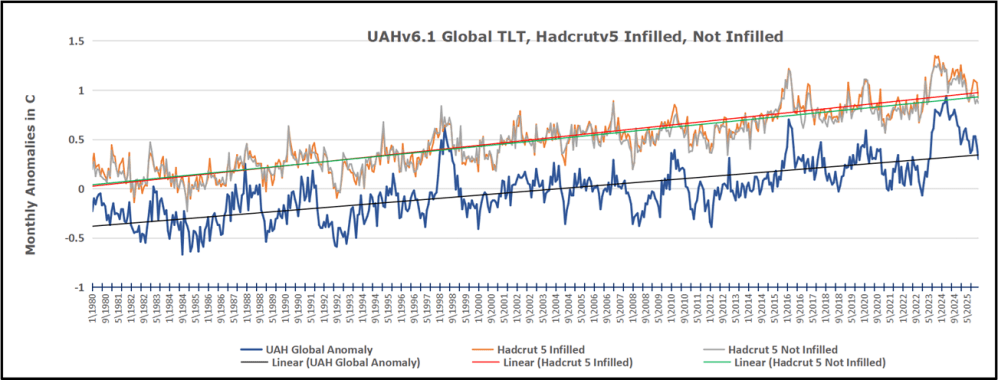
Just in time for COP30 in Belem, Brazil, we have fresh confirmation that cooling temperatures are resulting in lower than expected levels of atmospheric CO2. Historical records show that around 1875 was the coldest time in the last 10,000 years.  That was the end of the Little Ice Age, and since then temperatures have warmed at an average rate of about 0.5C per century.  The recovery of the biosphere and ocean warming resulted in rising levels of CO2 in the atmosphere. At times, there are warming spikes, in the 1930s and 40s for example, and the rate of rising CO2 goes up. At other times, such as 1950s and 60s, temperatures cool, and rising CO2 slows down. More recently, in 2023 and 24, we saw  temperatures spike up before falling back down in 2025.

Previously I have demonstrated that changes in atmospheric CO2 levels follow changes in Global Mean Temperatures (GMT) as shown by satellite measurements from University of Alabama at Huntsville (UAH). That background post is reprinted later below.

My curiosity was piqued by the remarkable GMT spike starting in January 2023 and rising to a peak in April 2024. GMT has declined steadily, and now 18 months later, the anomaly is 0.53C down from 0.94C.  I also became aware that UAH has recalibrated their dataset due to a satellite drift that can no longer be corrected. The values since 2020 have shifted slightly in version 6.1, as shown in my recent report UAH Ocean Stays Cool, SH Land Warms, October 2025, The data here comes from UAH record of temperatures measured in the lower troposphere (TLT).

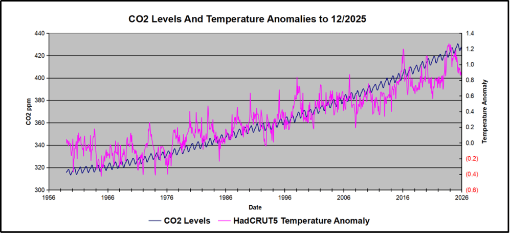
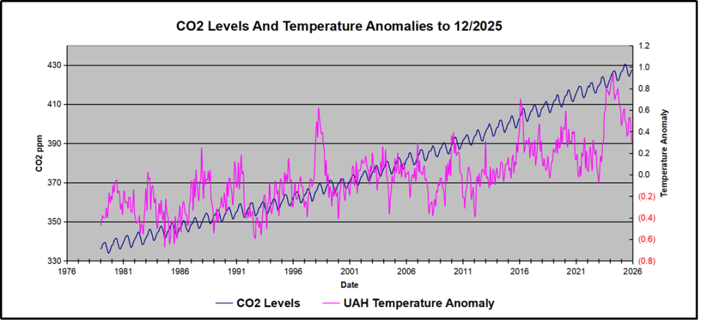
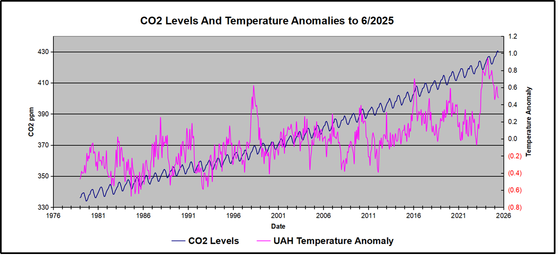
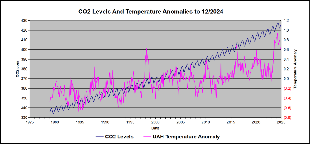
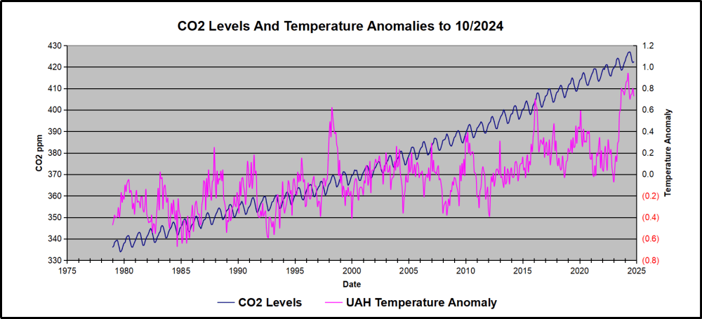
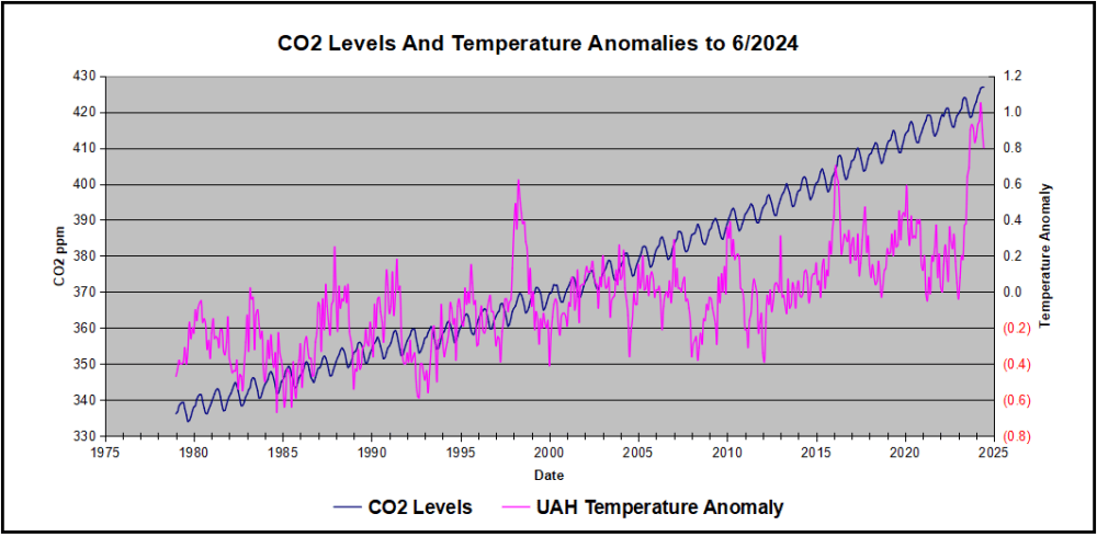
In this post, I test the premise that temperature changes are predictive of changes in atmospheric CO2 concentrations.  The chart above shows the two monthly datasets: CO2 levels in blue reported at Mauna Loa, and Global temperature anomalies in purple reported by UAHv6.1, both through October 2025. Would such a sharp increase in temperature be reflected in rising CO2 levels, according to the successful mathematical forecasting model? Would CO2 levels decline as temperatures dropped following the peak?

The answer is yes: that temperature spike resulted
in a corresponding CO2 spike as expected.
And lower CO2 levels followed the temperature decline.
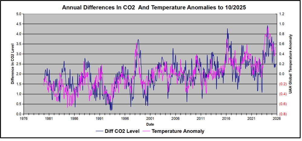
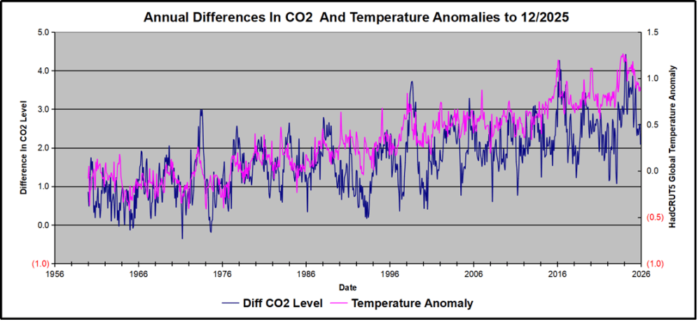
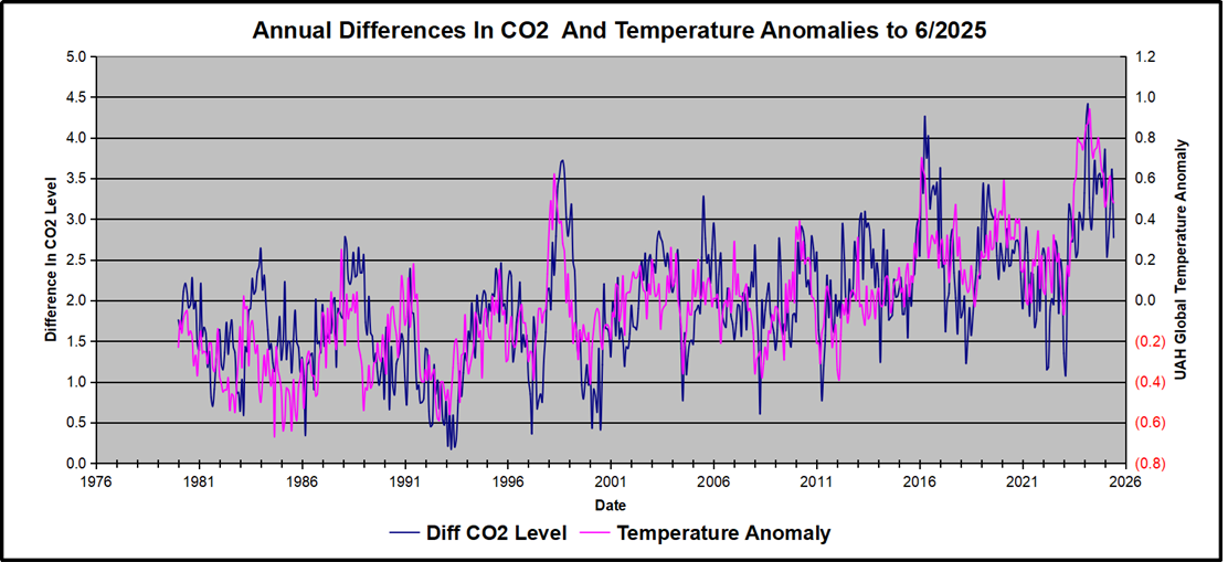
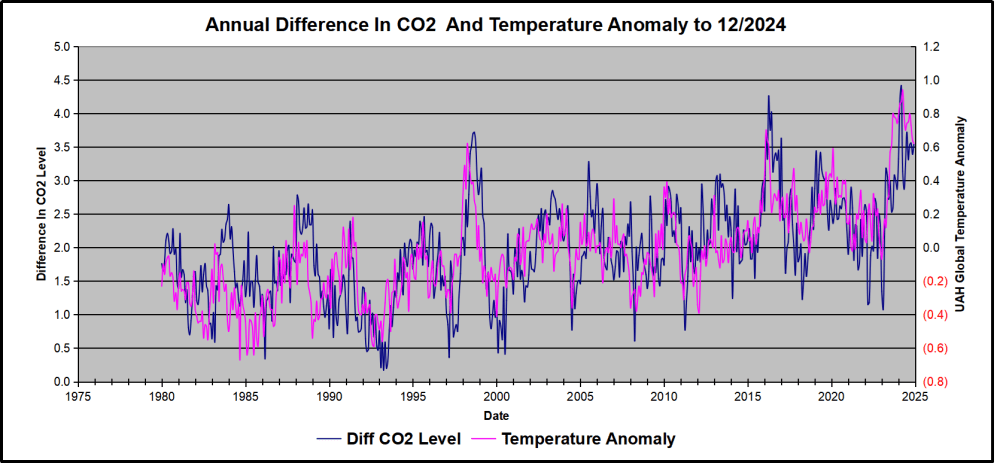
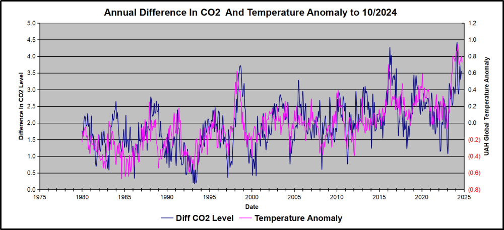
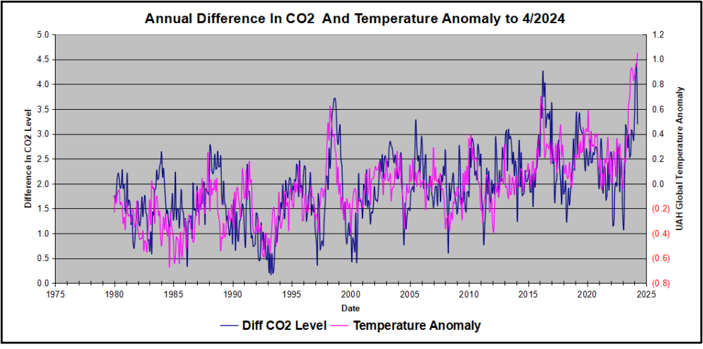
Above are UAH temperature anomalies compared to CO2 monthly changes year over year.

Changes in monthly CO2 synchronize with temperature fluctuations, which for UAH are anomalies referenced to the 1991-2020 period. CO2 differentials are calculated for the present month by subtracting the value for the same month in the previous year (for example October 2025 minus October 2024).  Temp anomalies are calculated by comparing the present month with the baseline month. Note the recent CO2 upward spike and drop following the temperature spike and drop.

The final proof that CO2 follows temperature due to stimulation of natural CO2 reservoirs is demonstrated by the ability to calculate CO2 levels since 1979 with a simple mathematical formula:

For each subsequent year, the CO2 level for each month was generated

CO2  this month this year = a + b × Temp this month this year  + CO2 this month last year

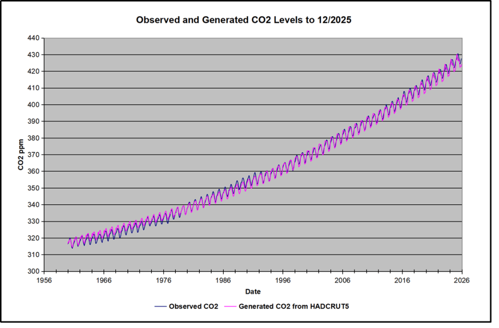
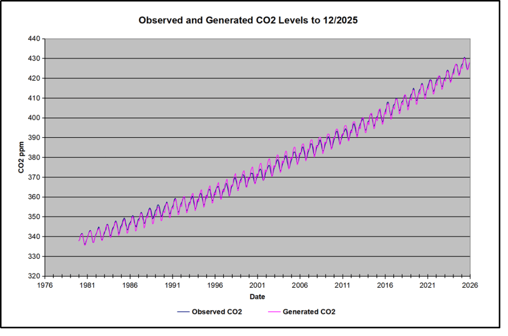
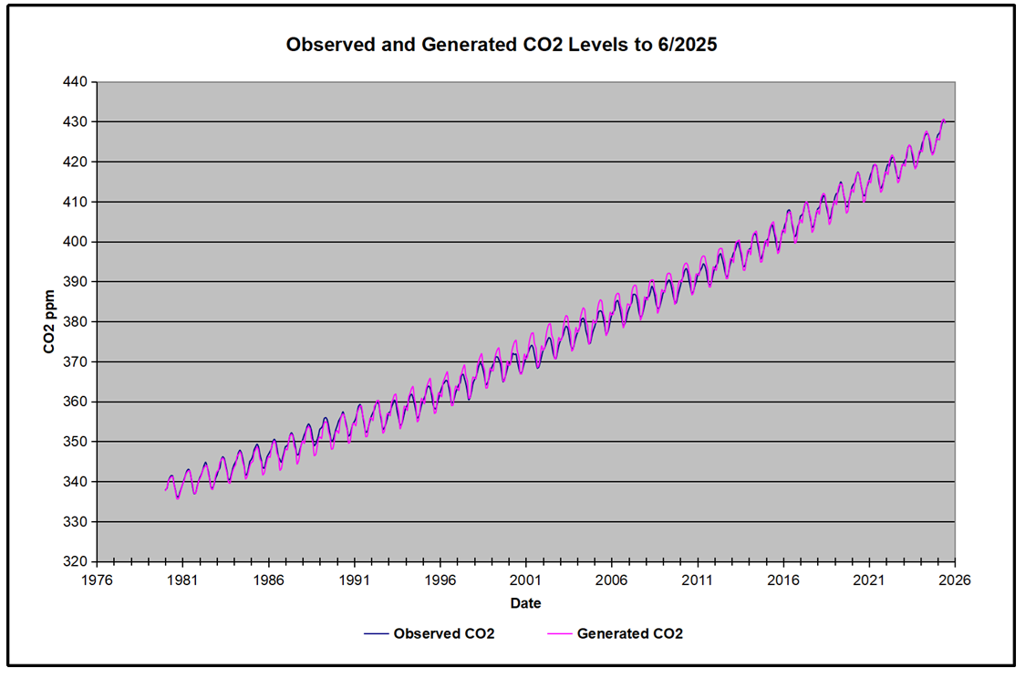
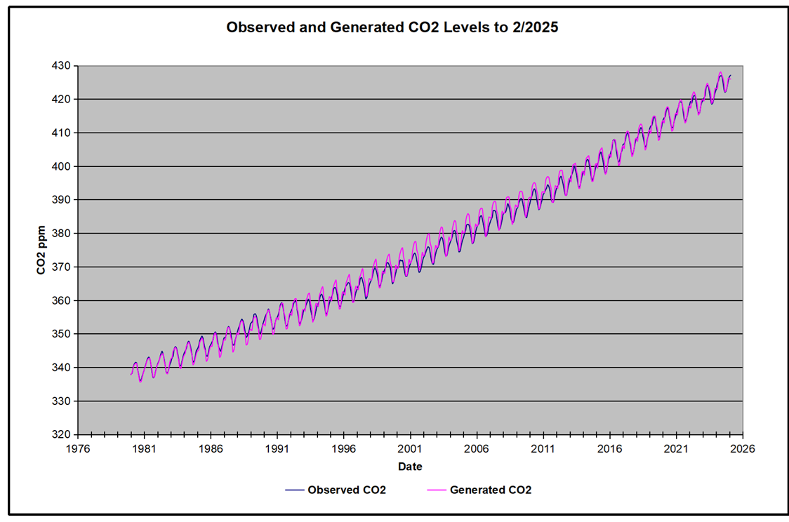
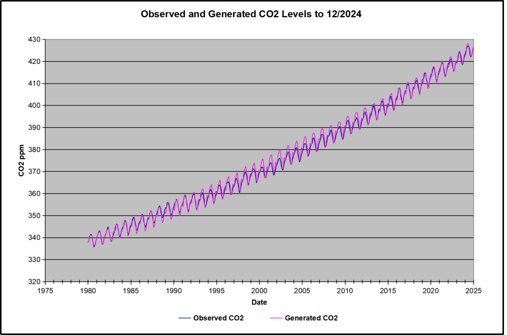
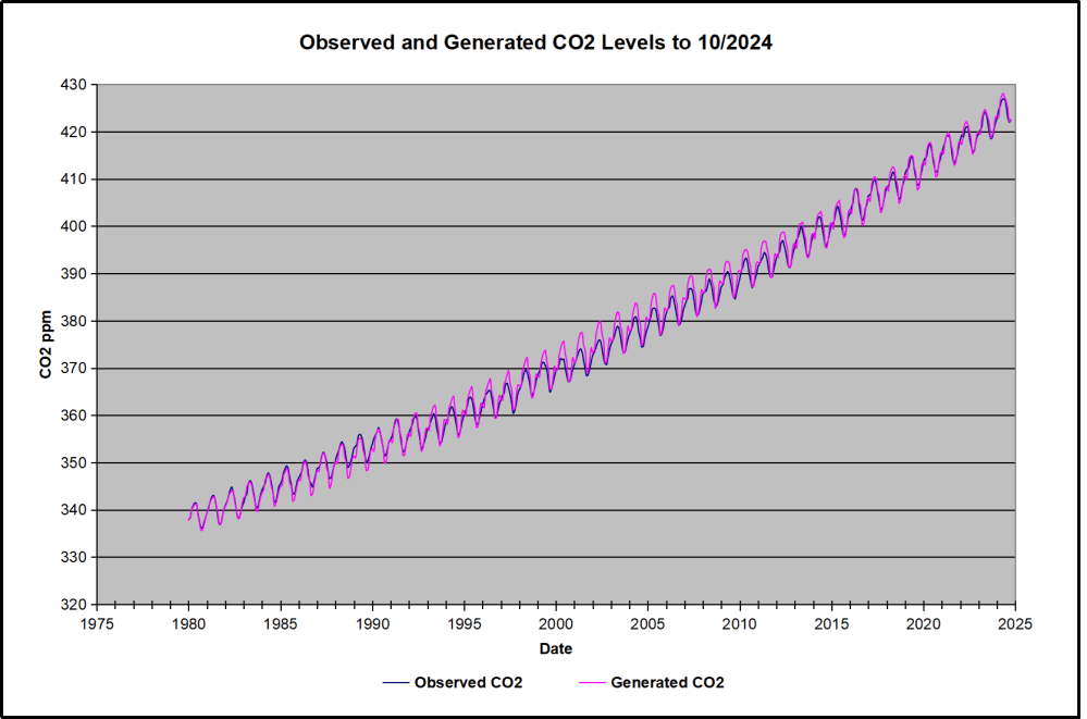
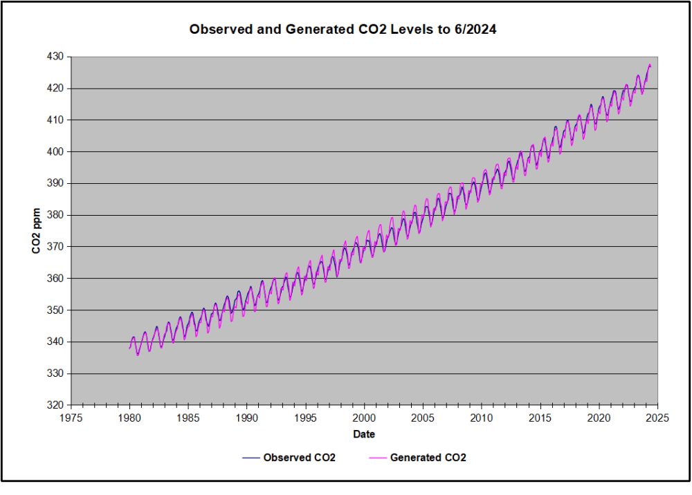
The values for a and b are constants applied to all monthly temps, and are chosen to scale the forecasted CO2 level for comparison with the observed value. Here is the result of those calculations.
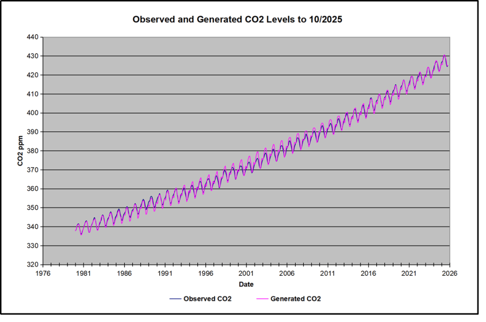
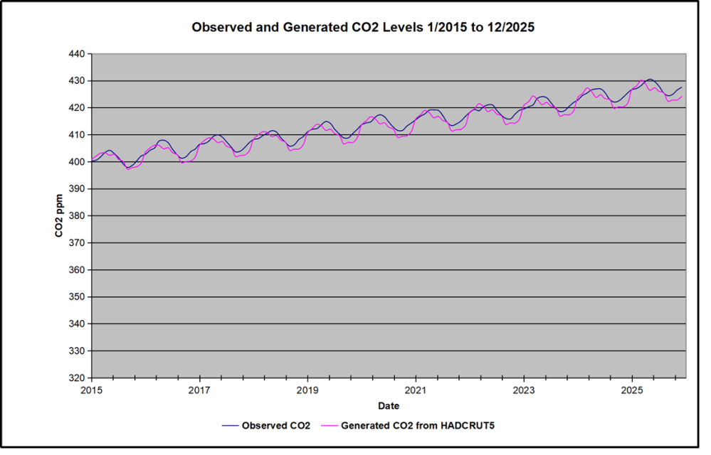
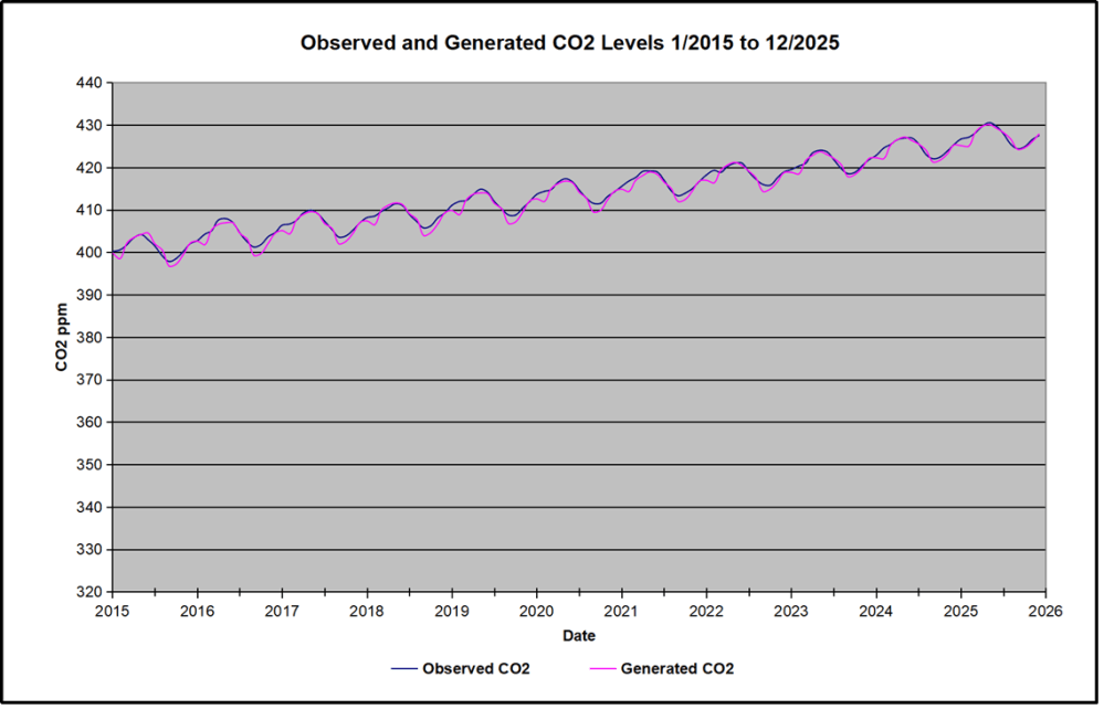
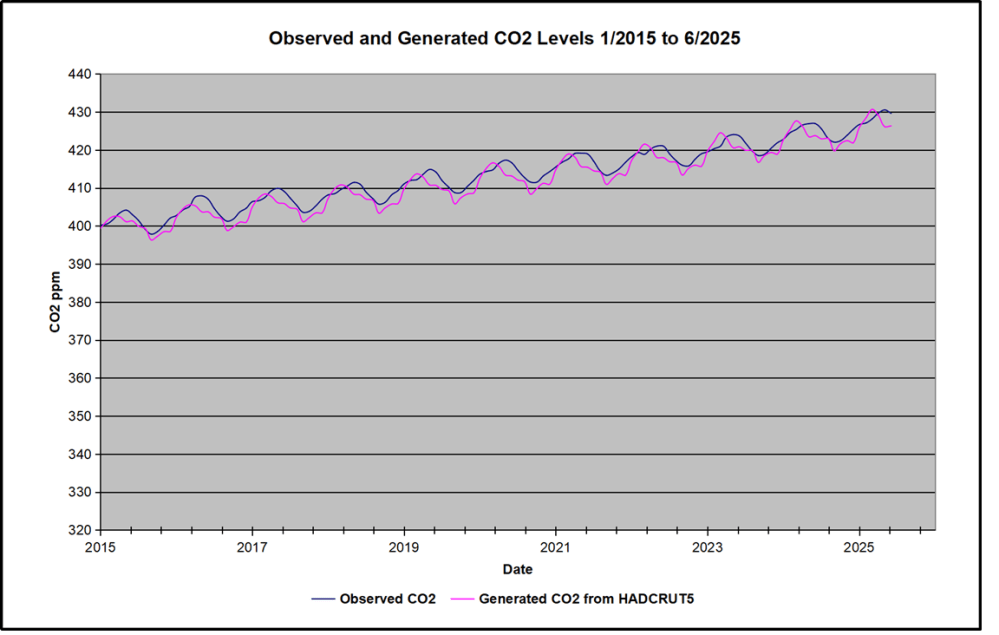
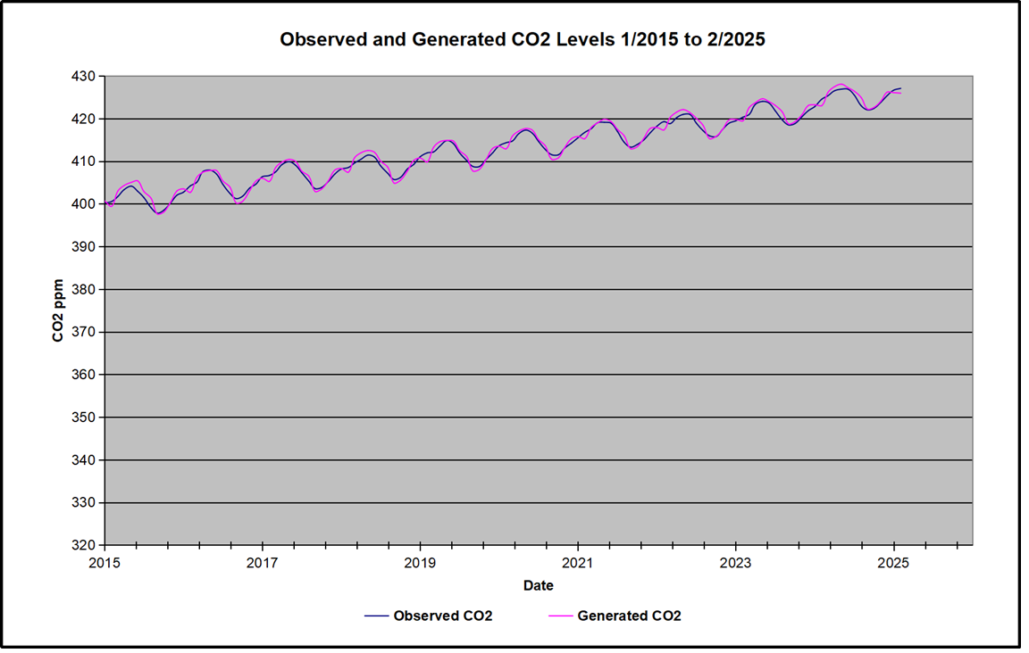
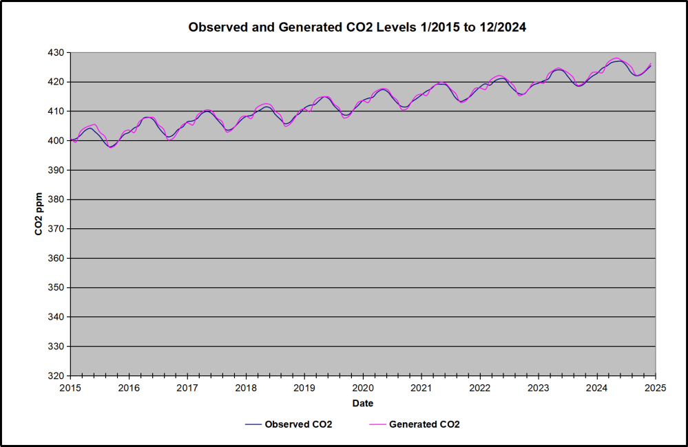
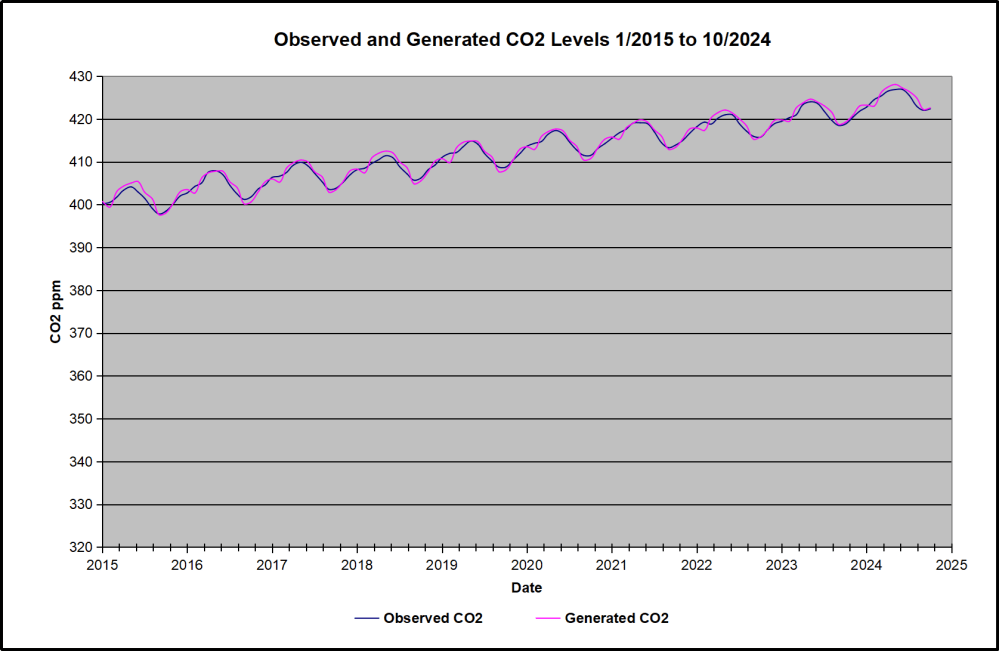
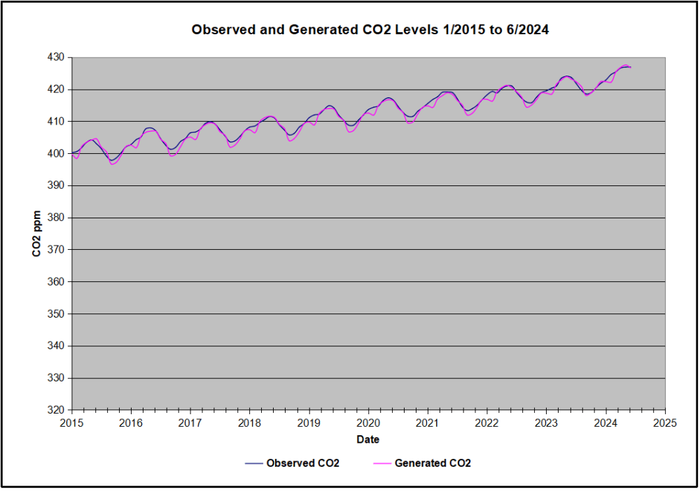
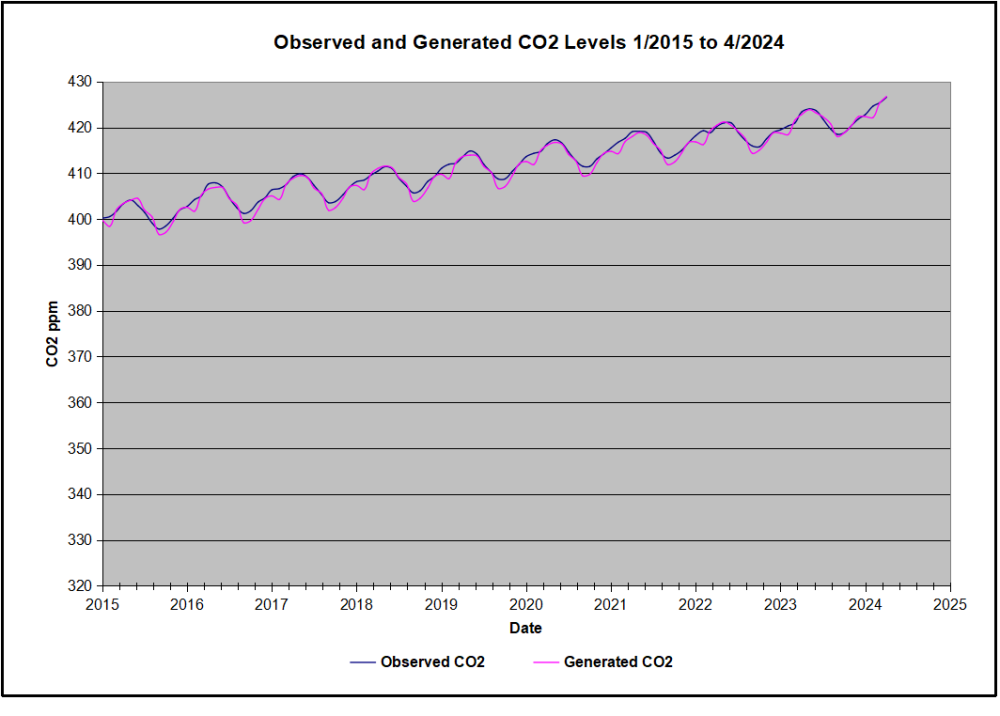
In the chart calculated CO2 levels correlate with observed CO2 levels at 0.9988 out of 1.0000.  This mathematical generation of CO2 atmospheric levels is only possible if they are driven by temperature-dependent natural sources, and not by human emissions which are small in comparison, rise steadily and monotonically.  For a more detailed look at the recent fluxes, here are the results since 2015, an ENSO neutral year.
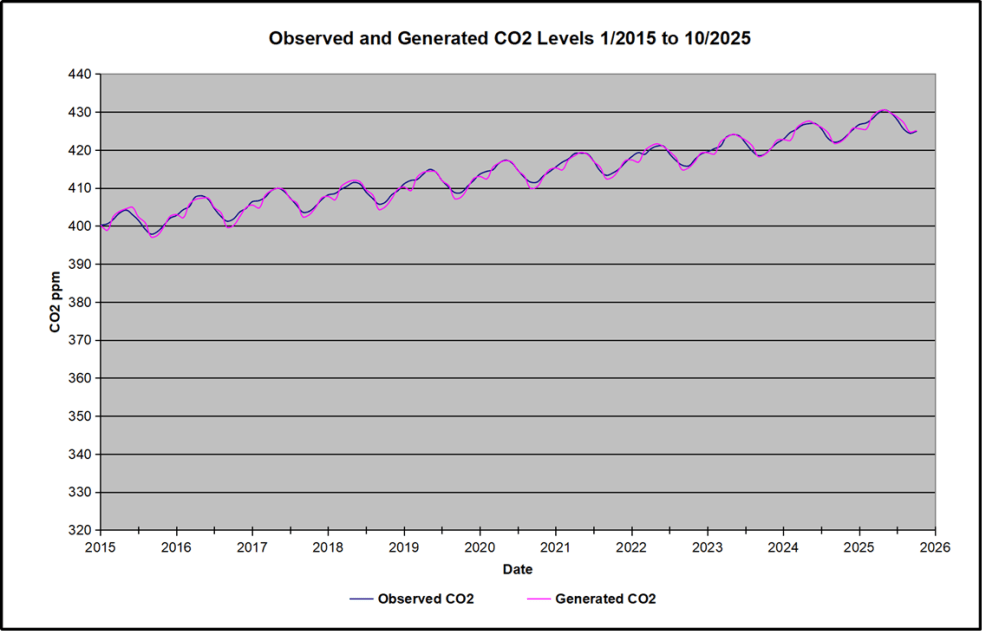
For this recent period, the calculated CO2 values match well the annual highs, while some annual generated values of CO2 are slightly higher or lower than observed at other months of the year. Still the correlation for this period is 0.9941.

Key Point

Changes in CO2 follow changes in global temperatures on all time scales, from last month’s observations to ice core datasets spanning millennia. Since CO2 is the lagging variable, it cannot logically be the cause of temperature, the leading variable. It is folly to imagine that by reducing human emissions of CO2, we can change global temperatures, which are obviously driven by other factors.
Background Post Temperature Changes Cause CO2 Changes, Not the Reverse

This post is about proving that CO2 changes in response to temperature changes, not the other way around, as is often claimed.  In order to do  that we need two datasets: one for measurements of changes in atmospheric CO2 concentrations over time and one for estimates of Global Mean Temperature changes over time.

Climate science is unsettling because past data are not fixed, but change later on.  I ran into this previously in 2021 and 2022 when I set out to update an analysis done in 2014 by Jeremy Shiers (discussed in a previous post reprinted at the end).  Jeremy provided a spreadsheet in his essay Murray Salby Showed CO2 Follows Temperature Now You Can Too posted in January 2014. I downloaded his spreadsheet intending to bring the analysis up to the present to see if the results hold up.  The two sources of data were:

Temperature anomalies from RSS here:  http://www.remss.com/missions/amsu

CO2 monthly levels from NOAA (Mauna Loa): https://www.esrl.noaa.gov/gmd/ccgg/trends/data.html

Changes in CO2 (ΔCO2)

Uploading the CO2 dataset showed that many numbers had changed (why?).
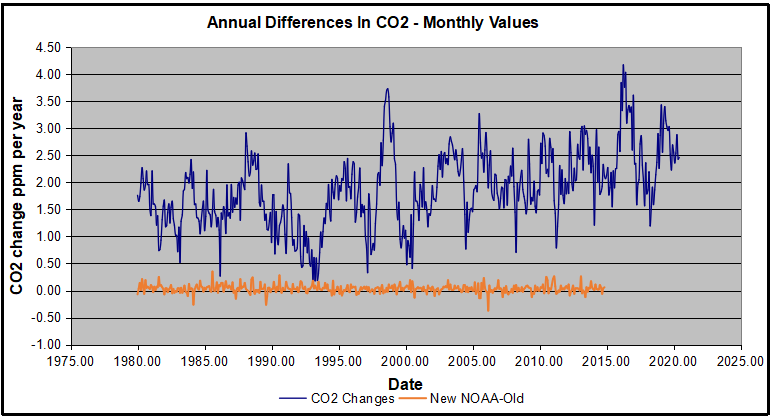
The blue line shows annual observed differences in monthly values year over year, e.g. June 2020 minus June 2019 etc.  The first 12 months (1979) provide the observed starting values from which differentials are calculated.  The orange line shows those CO2 values changed slightly in the 2020 dataset vs. the 2014 dataset, on average +0.035 ppm.  But there is no pattern or trend added, and deviations vary randomly between + and -.  So last year I took the 2020 dataset to replace the older one for updating the analysis.

Now I find the NOAA dataset starting in 2021 has almost completely new values due to a method shift in February 2021, requiring a recalibration of all previous measurements.  The new picture of ΔCO2 is graphed below.
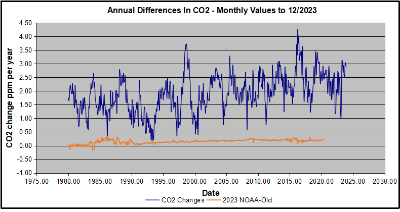
The method shift is reported at a NOAA Global Monitoring Laboratory webpage, Carbon Dioxide (CO2) WMO Scale, with a justification for the difference between X2007 results and the new results from X2019 now in force.  The orange line shows that the shift has resulted in higher values, especially early on and a general slightly increasing trend over time.  However, these are small variations at the decimal level on values 340 and above.  Further, the graph shows that yearly differentials month by month are virtually the same as before.  Thus I redid the analysis with the new values.

Global Temperature Anomalies (ΔTemp)

The other time series was the record of global temperature anomalies according to RSS. The current RSS dataset is not at all the same as the past.
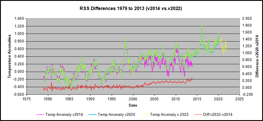
Here we see some seriously unsettling science at work.  The purple line is RSS in 2014, and the blue is RSS as of 2020.  Some further increases appear in the gold 2022 rss dataset. The red line shows alterations from the old to the new.  There is a slight cooling of the data in the beginning years, then the three versions mostly match until 1997, when systematic warming enters the record.  From 1997/5 to 2003/12 the average anomaly increases by 0.04C.  After 2004/1 to 2012/8 the average increase is 0.15C.  At the end from 2012/9 to 2013/12, the average anomaly was higher by 0.21. The 2022 version added slight warming over 2020 values.

RSS continues that accelerated warming to the present, but it cannot be trusted.  And who knows what the numbers will be a few years down the line?  As Dr. Ole Humlum said some years ago (regarding Gistemp): “It should however be noted, that a temperature record which keeps on changing the past hardly can qualify as being correct.”

Given the above manipulations, I went instead to the other satellite dataset UAH version 6. UAH has also made a shift by changing its baseline from 1981-2010 to 1991-2020.  This resulted in systematically reducing the anomaly values, but did not alter the pattern of variation over time.  For comparison, here are the two records with measurements through December 2023.

Comparing UAH temperature anomalies to NOAA CO2 changes.

Here are UAH temperature anomalies compared to CO2 monthly changes year over year.

Changes in monthly CO2 synchronize with temperature fluctuations, which for UAH are anomalies now referenced to the 1991-2020 period.  As stated above, CO2 differentials are calculated for the present month by subtracting the value for the same month in the previous year (for example June 2022 minus June 2021).   Temp anomalies are calculated by comparing the present month with the baseline month.

The final proof that CO2 follows temperature due to stimulation of natural CO2 reservoirs is demonstrated by the ability to calculate CO2 levels since 1979 with a simple mathematical formula:

For each subsequent year, the co2 level for each month was generated

CO2  this month this year = a + b × Temp this month this year  + CO2 this month last year

Jeremy used Python to estimate a and b, but I used his spreadsheet to guess values that place for comparison the observed and calculated CO2 levels on top of each other.

In the chart calculated CO2 levels correlate with observed CO2 levels at 0.9986 out of 1.0000.  This mathematical generation of CO2 atmospheric levels is only possible if they are driven by temperature-dependent natural sources, and not by human emissions which are small in comparison, rise steadily and monotonically.

Comment:  UAH dataset reported a sharp warming spike starting mid year, with causes speculated but not proven.  In any case, that surprising peak has not yet driven CO2 higher, though it might,  but only if it persists despite the likely cooling already under way.

Previous Post:  What Causes Rising Atmospheric CO2?
nasa_carbon_cycle_2008-1

This post is prompted by a recent exchange with those reasserting the “consensus” view attributing all additional atmospheric CO2 to humans burning fossil fuels.

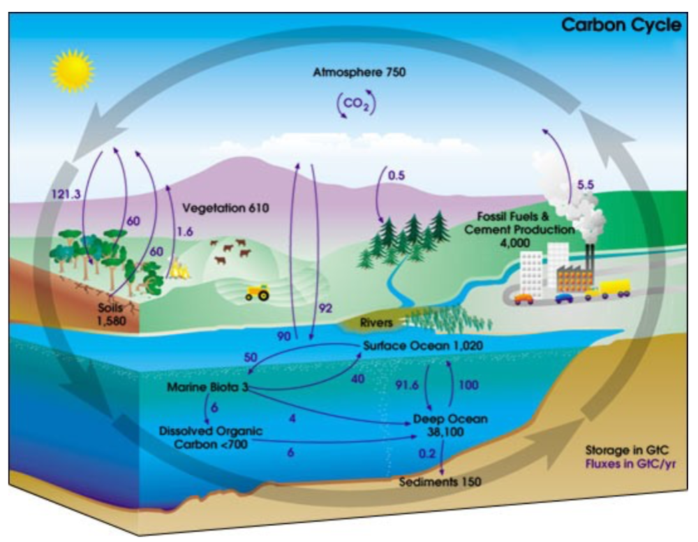
The IPCC doctrine which has long been promoted goes as follows. We have a number over here for monthly fossil fuel CO2 emissions, and a number over there for monthly atmospheric CO2. We don’t have good numbers for the rest of it-oceans, soils, biosphere–though rough estimates are orders of magnitude higher, dwarfing human CO2.  So we ignore nature and assume it is always a sink, explaining the difference between the two numbers we do have. Easy peasy, science settled.

What about the fact that nature continues to absorb about half of human emissions, even while FF CO2 increased by 60% over the last 2 decades? What about the fact that in 2020 FF CO2 declined significantly with no discernable impact on rising atmospheric CO2?

These and other issues are raised by Murray Salby and others who conclude that it is not that simple, and the science is not settled. And so these dissenters must be cancelled lest the narrative be weakened.

The non-IPCC paradigm is that atmospheric CO2 levels are a function of two very different fluxes. FF CO2 changes rapidly and increases steadily, while Natural CO2 changes slowly over time, and fluctuates up and down from temperature changes. The implications are that human CO2 is a simple addition, while natural CO2 comes from the integral of previous fluctuations.  Jeremy Shiers has a series of posts at his blog clarifying this paradigm. See Increasing CO2 Raises Global Temperature Or Does Increasing Temperature Raise CO2 Excerpts in italics with my bolds.

The following graph which shows the change in CO2 levels (rather than the levels directly) makes this much clearer.

Note the vertical scale refers to the first differential of the CO2 level not the level itself. The graph depicts that change rate in ppm per year.

There are big swings in the amount of CO2 emitted. Taking the mean as 1.6 ppmv/year (at a guess) there are +/- swings of around 1.2 nearly +/- 100%.

And, surprise surprise, the change in net emissions of CO2 is very strongly correlated with changes in global temperature.

This clearly indicates the net amount of CO2 emitted in any one year is directly linked to global mean temperature in that year.

For any given year the amount of CO2 in the atmosphere will be the sum of

  • all the net annual emissions of CO2
  • in all previous years.

For each year the net annual emission of CO2 is proportional to the annual global mean temperature.

This means the amount of CO2 in the atmosphere will be related to the sum of temperatures in previous years.

So CO2 levels are not directly related to the current temperature but the integral of temperature over previous years.

The following graph again shows observed levels of CO2 and global temperatures but also has calculated levels of CO2 based on sum of previous years temperatures (dotted blue line).

Summary:

The massive fluxes from natural sources dominate the flow of CO2 through the atmosphere.  Human CO2 from burning fossil fuels is around 4% of the annual addition from all sources. Even if rising CO2 could cause rising temperatures (no evidence, only claims), reducing our emissions would have little impact.

Atmospheric CO2 Math

Ins: 4% human, 96% natural
Outs: 0% human, 98% natural.
Atmospheric storage difference: +2%
(so that: Ins = Outs + Atmospheric storage difference)

Balance = Atmospheric storage difference: 2%, of which,
Humans: 2% X 4% = 0.08%
Nature: 2% X 96 % = 1.92%

Ratio Natural : Human =1.92% : 0.08% = 24 : 1

Resources
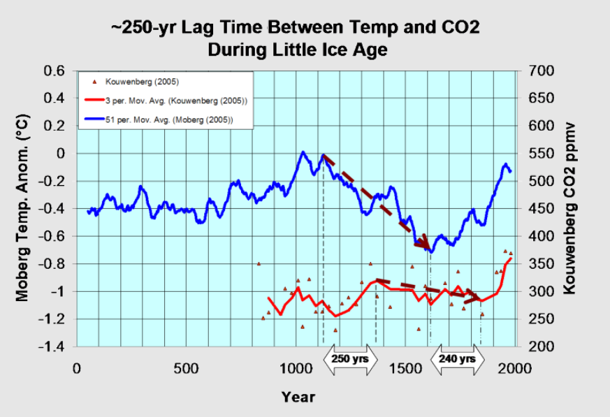
For a possible explanation of natural warming and CO2 emissions see Little Ice Age Warming Recovery May be Over
Resources:

CO2 Fluxes, Sources and Sinks

Who to Blame for Rising CO2?

Fearless Physics from Dr. Salby
ML CO2 Follows Temperatures From HadCRUT5

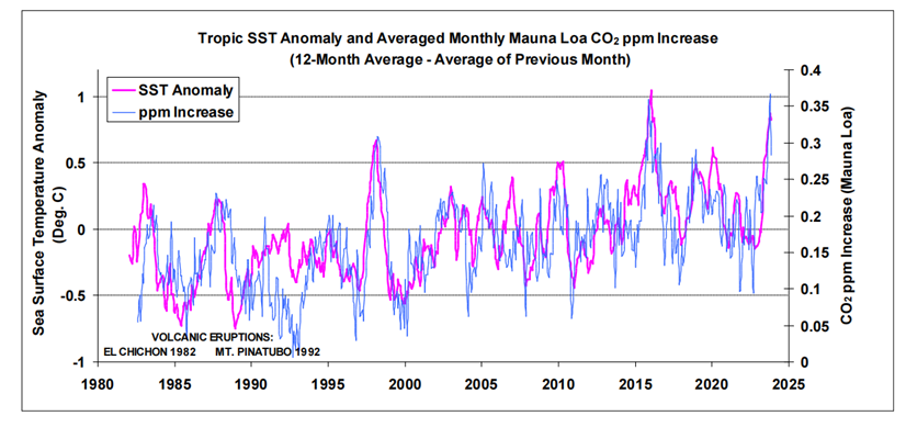
Previously I have demonstrated that temperature changes are predictive of changes in atmospheric CO2 concentrations.  That includes the remarkable GMT spike starting in January 2023 and rising to a peak in April 2024.  The most recent study was June 2025 Update–Temperature Falls, CO2 Follows employing Mauna Loa CO2 data and UAH GMT data.

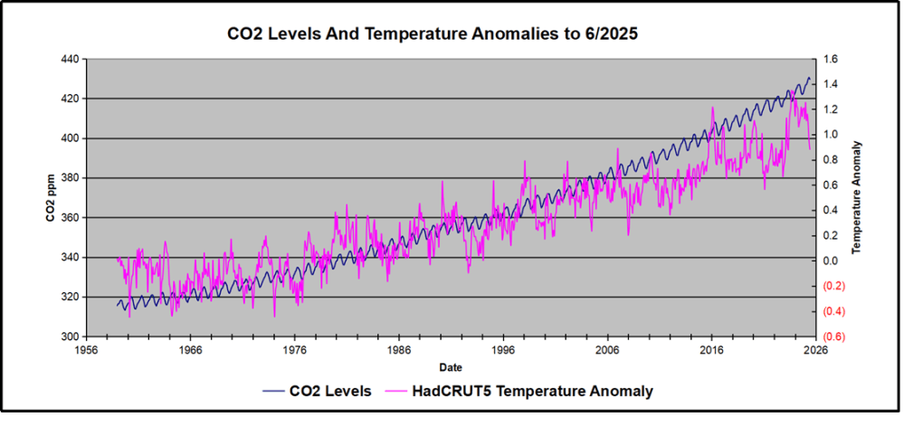
More recently another researcher, Bernard Robbins, found similar causation between ML CO2 and SST fluctuations reported by NOAA Global SST dataset.  See More Evidence Temperatures Drive CO2 Levels, Not the Reverse.    Along with some comments on my blog, I wondered whether the entire ML record of CO2 levels could be predicted from global temperature changes, which would require a GMT dataset covering 1959 to the present.  This post shows that HADCRUT5 qualifies and indeed confirms other studies by researchers. I was particularly interested in the lack of warming in the 1960s and 70s, before the satellite temperature data became available.

The answer is yes: Just as temperature spikes result
in a corresponding CO2 spike as expected.  Cooler temperatures
are predictive of lower CO2 levels.

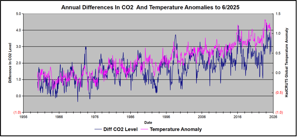
Above are HadCRUT5 temperature anomalies compared to CO2 monthly changes year over year.

Changes in monthly CO2 synchronize with temperature fluctuations, which for HadCRUT5 are anomalies referenced to the 1961-1990 period. CO2 differentials are calculated for the present month by subtracting the value for the same month in the previous year (for example February 2025 minus February 2024).  Temp anomalies are calculated by comparing the present month with the baseline month. Note the recent CO2 upward spike and drop following the temperature spike and drop.

The final proof that CO2 follows temperature due to stimulation of natural CO2 reservoirs is demonstrated by the ability to calculate CO2 levels since 1959 with a simple mathematical formula:

For each subsequent year, the CO2 level for each month was generated

CO2  this month this year = a + b × Temp this month this year  + CO2 this month last year

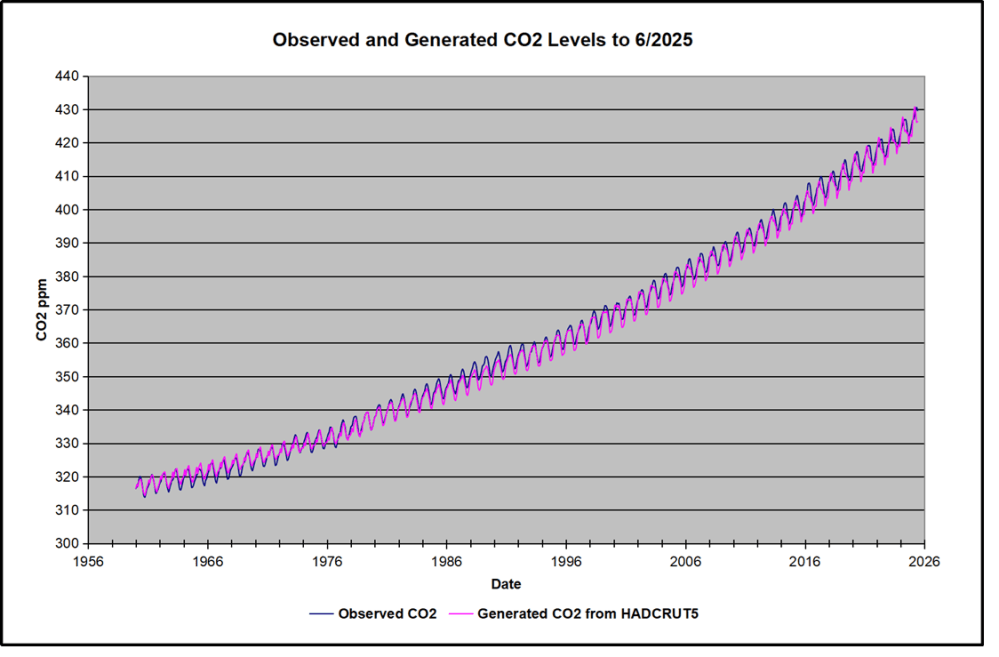
The values for a and b are constants applied to all monthly temps, and are chosen to scale the forecasted CO2 level for comparison with the observed value. The values for scaling HADCRUT5 and MLCO2 were “a” = 1.12 and “b” = 1.65 Here is the result of those calculations.

In the chart calculated CO2 levels correlate with observed CO2 levels at 0.9992 out of 1.0000.  This mathematical generation of CO2 atmospheric levels is only possible if they are driven by temperature-dependent natural sources, and not by human emissions which are small in comparison, rise steadily and monotonically.  For a more detailed look at the recent fluxes, here are the results since 2015, an ENSO neutral year.

For this recent period, the calculated CO2 values match well the annual lows, while some annual generated values of CO2 are slightly higher or lower than observed at other months of the year. Still the correlation for this period is 0.98

Key Point

Changes in CO2 follow changes in global temperatures on all time scales, from last month’s observations to ice core datasets spanning millennia. Since CO2 is the lagging variable, it cannot logically be the cause of temperature, the leading variable. It is folly to imagine that by reducing human emissions of CO2, we can change global temperatures, which are obviously driven by other factors.

Background Post Temperature Changes Cause CO2 Changes, Not the Reverse

This post is about proving that CO2 changes in response to temperature changes, not the other way around, as is often claimed.  In order to do  that we need two datasets: one for measurements of changes in atmospheric CO2 concentrations over time and one for estimates of Global Mean Temperature changes over time.

Climate science is unsettling because past data are not fixed, but change later on.  I ran into this previously and now again in 2021 and 2022 when I set out to update an analysis done in 2014 by Jeremy Shiers (discussed in a previous post reprinted at the end).  Jeremy provided a spreadsheet in his essay Murray Salby Showed CO2 Follows Temperature Now You Can Too posted in January 2014. I downloaded his spreadsheet intending to bring the analysis up to the present to see if the results hold up.  The two sources of data were:

Temperature anomalies from RSS here:  http://www.remss.com/missions/amsu

CO2 monthly levels from NOAA (Mauna Loa): https://www.esrl.noaa.gov/gmd/ccgg/trends/data.html

Changes in CO2 (ΔCO2)

Uploading the CO2 dataset showed that many numbers had changed (why?).

The blue line shows annual observed differences in monthly values year over year, e.g. June 2020 minus June 2019 etc.  The first 12 months (1979) provide the observed starting values from which differentials are calculated.  The orange line shows those CO2 values changed slightly in the 2020 dataset vs. the 2014 dataset, on average +0.035 ppm.  But there is no pattern or trend added, and deviations vary randomly between + and -.  So last year I took the 2020 dataset to replace the older one for updating the analysis.

Now I find the NOAA dataset starting in 2021 has almost completely new values due to a method shift in February 2021, requiring a recalibration of all previous measurements.  The new picture of ΔCO2 is graphed below.

The method shift is reported at a NOAA Global Monitoring Laboratory webpage, Carbon Dioxide (CO2) WMO Scale, with a justification for the difference between X2007 results and the new results from X2019 now in force.  The orange line shows that the shift has resulted in higher values, especially early on and a general slightly increasing trend over time.  However, these are small variations at the decimal level on values 340 and above.  Further, the graph shows that yearly differentials month by month are virtually the same as before.  Thus I redid the analysis with the new values.

Global Temperature Anomalies (ΔTemp)

The other time series was the record of global temperature anomalies according to RSS. The current RSS dataset is not at all the same as the past.

Here we see some seriously unsettling science at work.  The purple line is RSS in 2014, and the blue is RSS as of 2020.  Some further increases appear in the gold 2022 rss dataset. The red line shows alterations from the old to the new.  There is a slight cooling of the data in the beginning years, then the three versions mostly match until 1997, when systematic warming enters the record.  From 1997/5 to 2003/12 the average anomaly increases by 0.04C.  After 2004/1 to 2012/8 the average increase is 0.15C.  At the end from 2012/9 to 2013/12, the average anomaly was higher by 0.21. The 2022 version added slight warming over 2020 values.

RSS continues that accelerated warming to the present, but it cannot be trusted.  And who knows what the numbers will be a few years down the line?  As Dr. Ole Humlum said some years ago (regarding Gistemp): “It should however be noted, that a temperature record which keeps on changing the past hardly can qualify as being correct.”

Given the above manipulations, I went instead to the other satellite dataset UAH version 6. UAH has also made a shift by changing its baseline from 1981-2010 to 1991-2020.  This resulted in systematically reducing the anomaly values, but did not alter the pattern of variation over time.  For comparison, here are the two records with measurements through December 2023.

Comparing UAH temperature anomalies to NOAA CO2 changes.

Here are UAH temperature anomalies compared to CO2 monthly changes year over year.

Changes in monthly CO2 synchronize with temperature fluctuations, which for UAH are anomalies now referenced to the 1991-2020 period.  As stated above, CO2 differentials are calculated for the present month by subtracting the value for the same month in the previous year (for example June 2022 minus June 2021).   Temp anomalies are calculated by comparing the present month with the baseline month.

The final proof that CO2 follows temperature due to stimulation of natural CO2 reservoirs is demonstrated by the ability to calculate CO2 levels since 1979 with a simple mathematical formula:

For each subsequent year, the co2 level for each month was generated

CO2  this month this year = a + b × Temp this month this year  + CO2 this month last year

Jeremy used Python to estimate a and b, but I used his spreadsheet to guess values that place for comparison the observed and calculated CO2 levels on top of each other.

In the chart calculated CO2 levels correlate with observed CO2 levels at 0.9986 out of 1.0000.  This mathematical generation of CO2 atmospheric levels is only possible if they are driven by temperature-dependent natural sources, and not by human emissions which are small in comparison, rise steadily and monotonically.

Comment:  UAH dataset reported a sharp warming spike starting mid year, with causes speculated but not proven.  In any case, that surprising peak has not yet driven CO2 higher, though it might,  but only if it persists despite the likely cooling already under way.

Previous Post:  What Causes Rising Atmospheric CO2?

nasa_carbon_cycle_2008-1

This post is prompted by a recent exchange with those reasserting the “consensus” view attributing all additional atmospheric CO2 to humans burning fossil fuels.

The IPCC doctrine which has long been promoted goes as follows. We have a number over here for monthly fossil fuel CO2 emissions, and a number over there for monthly atmospheric CO2. We don’t have good numbers for the rest of it-oceans, soils, biosphere–though rough estimates are orders of magnitude higher, dwarfing human CO2.  So we ignore nature and assume it is always a sink, explaining the difference between the two numbers we do have. Easy peasy, science settled.

What about the fact that nature continues to absorb about half of human emissions, even while FF CO2 increased by 60% over the last 2 decades? What about the fact that in 2020 FF CO2 declined significantly with no discernable impact on rising atmospheric CO2?

These and other issues are raised by Murray Salby and others who conclude that it is not that simple, and the science is not settled. And so these dissenters must be cancelled lest the narrative be weakened.

The non-IPCC paradigm is that atmospheric CO2 levels are a function of two very different fluxes. FF CO2 changes rapidly and increases steadily, while Natural CO2 changes slowly over time, and fluctuates up and down from temperature changes. The implications are that human CO2 is a simple addition, while natural CO2 comes from the integral of previous fluctuations.  Jeremy Shiers has a series of posts at his blog clarifying this paradigm. See Increasing CO2 Raises Global Temperature Or Does Increasing Temperature Raise CO2 Excerpts in italics with my bolds.

The following graph which shows the change in CO2 levels (rather than the levels directly) makes this much clearer.

Note the vertical scale refers to the first differential of the CO2 level not the level itself. The graph depicts that change rate in ppm per year.

There are big swings in the amount of CO2 emitted. Taking the mean as 1.6 ppmv/year (at a guess) there are +/- swings of around 1.2 nearly +/- 100%.

And, surprise surprise, the change in net emissions of CO2 is very strongly correlated with changes in global temperature.

This clearly indicates the net amount of CO2 emitted in any one year is directly linked to global mean temperature in that year.

For any given year the amount of CO2 in the atmosphere will be the sum of

  • all the net annual emissions of CO2
  • in all previous years.

For each year the net annual emission of CO2 is proportional to the annual global mean temperature.

This means the amount of CO2 in the atmosphere will be related to the sum of temperatures in previous years.

So CO2 levels are not directly related to the current temperature but the integral of temperature over previous years.

The following graph again shows observed levels of CO2 and global temperatures but also has calculated levels of CO2 based on sum of previous years temperatures (dotted blue line).

Summary:

The massive fluxes from natural sources dominate the flow of CO2 through the atmosphere.  Human CO2 from burning fossil fuels is around 4% of the annual addition from all sources. Even if rising CO2 could cause rising temperatures (no evidence, only claims), reducing our emissions would have little impact.

Atmospheric CO2 Math

Ins: 4% human, 96% natural
Outs: 0% human, 98% natural.
Atmospheric storage difference: +2%
(so that: Ins = Outs + Atmospheric storage difference)

Balance = Atmospheric storage difference: 2%, of which,
Humans: 2% X 4% = 0.08%
Nature: 2% X 96 % = 1.92%

Ratio Natural : Human =1.92% : 0.08% = 24 : 1

Resources
For a possible explanation of natural warming and CO2 emissions see Little Ice Age Warming Recovery May be Over
Resources:

CO2 Fluxes, Sources and Sinks

Who to Blame for Rising CO2?

Fearless Physics from Dr. Salby

June 2025 Update–Temperature Falls, CO2 Follows

Previously I have demonstrated that changes in atmospheric CO2 levels follow changes in Global Mean Temperatures (GMT) as shown by satellite measurements from University of Alabama at Huntsville (UAH). That background post is reprinted later below.

My curiosity was piqued by the remarkable GMT spike starting in January 2023 and rising to a peak in April 2024. GMT has declined steadily, and now 14 months later, the anomaly is 0.48C down from 0.94C.  I also became aware that UAH has recalibrated their dataset due to a satellite drift that can no longer be corrected. The values since 2020 have shifted slightly in version 6.1, as shown in my recent report NH and Tropics Lead UAH Temps Lower May 2025.  The data here comes from UAH record of temperatures measured in the lower troposphere (TLT).

In this post, I test the premise that temperature changes are predictive of changes in atmospheric CO2 concentrations.  The chart above shows the two monthly datasets: CO2 levels in blue reported at Mauna Loa, and Global temperature anomalies in purple reported by UAHv6.1, both through June 2025. Would such a sharp increase in temperature be reflected in rising CO2 levels, according to the successful mathematical forecasting model? Would CO2 levels decline as temperatures dropped following the peak?

The answer is yes: that temperature spike resulted
in a corresponding CO2 spike as expected.
And lower CO2 levels followed the temperature decline.

Above are UAH temperature anomalies compared to CO2 monthly changes year over year.

Changes in monthly CO2 synchronize with temperature fluctuations, which for UAH are anomalies referenced to the 1991-2020 period. CO2 differentials are calculated for the present month by subtracting the value for the same month in the previous year (for example February 2025 minus February 2024).  Temp anomalies are calculated by comparing the present month with the baseline month. Note the recent CO2 upward spike and drop following the temperature spike and drop.

The final proof that CO2 follows temperature due to stimulation of natural CO2 reservoirs is demonstrated by the ability to calculate CO2 levels since 1979 with a simple mathematical formula:

For each subsequent year, the CO2 level for each month was generated

CO2  this month this year = a + b × Temp this month this year  + CO2 this month last year

The values for a and b are constants applied to all monthly temps, and are chosen to scale the forecasted CO2 level for comparison with the observed value. Here is the result of those calculations.

In the chart calculated CO2 levels correlate with observed CO2 levels at 0.9988 out of 1.0000.  This mathematical generation of CO2 atmospheric levels is only possible if they are driven by temperature-dependent natural sources, and not by human emissions which are small in comparison, rise steadily and monotonically.  For a more detailed look at the recent fluxes, here are the results since 2015, an ENSO neutral year.

For this recent period, the calculated CO2 values match well the annual highs, while some annual generated values of CO2 are slightly higher or lower than observed at other months of the year. Still the correlation for this period is 0.9939.

Key Point

Changes in CO2 follow changes in global temperatures on all time scales, from last month’s observations to ice core datasets spanning millennia. Since CO2 is the lagging variable, it cannot logically be the cause of temperature, the leading variable. It is folly to imagine that by reducing human emissions of CO2, we can change global temperatures, which are obviously driven by other factors.

Background Post Temperature Changes Cause CO2 Changes, Not the Reverse

This post is about proving that CO2 changes in response to temperature changes, not the other way around, as is often claimed.  In order to do  that we need two datasets: one for measurements of changes in atmospheric CO2 concentrations over time and one for estimates of Global Mean Temperature changes over time.

Climate science is unsettling because past data are not fixed, but change later on.  I ran into this previously and now again in 2021 and 2022 when I set out to update an analysis done in 2014 by Jeremy Shiers (discussed in a previous post reprinted at the end).  Jeremy provided a spreadsheet in his essay Murray Salby Showed CO2 Follows Temperature Now You Can Too posted in January 2014. I downloaded his spreadsheet intending to bring the analysis up to the present to see if the results hold up.  The two sources of data were:

Temperature anomalies from RSS here:  http://www.remss.com/missions/amsu

CO2 monthly levels from NOAA (Mauna Loa): https://www.esrl.noaa.gov/gmd/ccgg/trends/data.html

Changes in CO2 (ΔCO2)

Uploading the CO2 dataset showed that many numbers had changed (why?).

The blue line shows annual observed differences in monthly values year over year, e.g. June 2020 minus June 2019 etc.  The first 12 months (1979) provide the observed starting values from which differentials are calculated.  The orange line shows those CO2 values changed slightly in the 2020 dataset vs. the 2014 dataset, on average +0.035 ppm.  But there is no pattern or trend added, and deviations vary randomly between + and -.  So last year I took the 2020 dataset to replace the older one for updating the analysis.

Now I find the NOAA dataset starting in 2021 has almost completely new values due to a method shift in February 2021, requiring a recalibration of all previous measurements.  The new picture of ΔCO2 is graphed below.

The method shift is reported at a NOAA Global Monitoring Laboratory webpage, Carbon Dioxide (CO2) WMO Scale, with a justification for the difference between X2007 results and the new results from X2019 now in force.  The orange line shows that the shift has resulted in higher values, especially early on and a general slightly increasing trend over time.  However, these are small variations at the decimal level on values 340 and above.  Further, the graph shows that yearly differentials month by month are virtually the same as before.  Thus I redid the analysis with the new values.

Global Temperature Anomalies (ΔTemp)

The other time series was the record of global temperature anomalies according to RSS. The current RSS dataset is not at all the same as the past.

Here we see some seriously unsettling science at work.  The purple line is RSS in 2014, and the blue is RSS as of 2020.  Some further increases appear in the gold 2022 rss dataset. The red line shows alterations from the old to the new.  There is a slight cooling of the data in the beginning years, then the three versions mostly match until 1997, when systematic warming enters the record.  From 1997/5 to 2003/12 the average anomaly increases by 0.04C.  After 2004/1 to 2012/8 the average increase is 0.15C.  At the end from 2012/9 to 2013/12, the average anomaly was higher by 0.21. The 2022 version added slight warming over 2020 values.

RSS continues that accelerated warming to the present, but it cannot be trusted.  And who knows what the numbers will be a few years down the line?  As Dr. Ole Humlum said some years ago (regarding Gistemp): “It should however be noted, that a temperature record which keeps on changing the past hardly can qualify as being correct.”

Given the above manipulations, I went instead to the other satellite dataset UAH version 6. UAH has also made a shift by changing its baseline from 1981-2010 to 1991-2020.  This resulted in systematically reducing the anomaly values, but did not alter the pattern of variation over time.  For comparison, here are the two records with measurements through December 2023.

Comparing UAH temperature anomalies to NOAA CO2 changes.

Here are UAH temperature anomalies compared to CO2 monthly changes year over year.

Changes in monthly CO2 synchronize with temperature fluctuations, which for UAH are anomalies now referenced to the 1991-2020 period.  As stated above, CO2 differentials are calculated for the present month by subtracting the value for the same month in the previous year (for example June 2022 minus June 2021).   Temp anomalies are calculated by comparing the present month with the baseline month.

The final proof that CO2 follows temperature due to stimulation of natural CO2 reservoirs is demonstrated by the ability to calculate CO2 levels since 1979 with a simple mathematical formula:

For each subsequent year, the co2 level for each month was generated

CO2  this month this year = a + b × Temp this month this year  + CO2 this month last year

Jeremy used Python to estimate a and b, but I used his spreadsheet to guess values that place for comparison the observed and calculated CO2 levels on top of each other.

In the chart calculated CO2 levels correlate with observed CO2 levels at 0.9986 out of 1.0000.  This mathematical generation of CO2 atmospheric levels is only possible if they are driven by temperature-dependent natural sources, and not by human emissions which are small in comparison, rise steadily and monotonically.

Comment:  UAH dataset reported a sharp warming spike starting mid year, with causes speculated but not proven.  In any case, that surprising peak has not yet driven CO2 higher, though it might,  but only if it persists despite the likely cooling already under way.

Previous Post:  What Causes Rising Atmospheric CO2?

nasa_carbon_cycle_2008-1

This post is prompted by a recent exchange with those reasserting the “consensus” view attributing all additional atmospheric CO2 to humans burning fossil fuels.

The IPCC doctrine which has long been promoted goes as follows. We have a number over here for monthly fossil fuel CO2 emissions, and a number over there for monthly atmospheric CO2. We don’t have good numbers for the rest of it-oceans, soils, biosphere–though rough estimates are orders of magnitude higher, dwarfing human CO2.  So we ignore nature and assume it is always a sink, explaining the difference between the two numbers we do have. Easy peasy, science settled.

What about the fact that nature continues to absorb about half of human emissions, even while FF CO2 increased by 60% over the last 2 decades? What about the fact that in 2020 FF CO2 declined significantly with no discernable impact on rising atmospheric CO2?

These and other issues are raised by Murray Salby and others who conclude that it is not that simple, and the science is not settled. And so these dissenters must be cancelled lest the narrative be weakened.

The non-IPCC paradigm is that atmospheric CO2 levels are a function of two very different fluxes. FF CO2 changes rapidly and increases steadily, while Natural CO2 changes slowly over time, and fluctuates up and down from temperature changes. The implications are that human CO2 is a simple addition, while natural CO2 comes from the integral of previous fluctuations.  Jeremy Shiers has a series of posts at his blog clarifying this paradigm. See Increasing CO2 Raises Global Temperature Or Does Increasing Temperature Raise CO2 Excerpts in italics with my bolds.

The following graph which shows the change in CO2 levels (rather than the levels directly) makes this much clearer.

Note the vertical scale refers to the first differential of the CO2 level not the level itself. The graph depicts that change rate in ppm per year.

There are big swings in the amount of CO2 emitted. Taking the mean as 1.6 ppmv/year (at a guess) there are +/- swings of around 1.2 nearly +/- 100%.

And, surprise surprise, the change in net emissions of CO2 is very strongly correlated with changes in global temperature.

This clearly indicates the net amount of CO2 emitted in any one year is directly linked to global mean temperature in that year.

For any given year the amount of CO2 in the atmosphere will be the sum of

  • all the net annual emissions of CO2
  • in all previous years.

For each year the net annual emission of CO2 is proportional to the annual global mean temperature.

This means the amount of CO2 in the atmosphere will be related to the sum of temperatures in previous years.

So CO2 levels are not directly related to the current temperature but the integral of temperature over previous years.

The following graph again shows observed levels of CO2 and global temperatures but also has calculated levels of CO2 based on sum of previous years temperatures (dotted blue line).

Summary:

The massive fluxes from natural sources dominate the flow of CO2 through the atmosphere.  Human CO2 from burning fossil fuels is around 4% of the annual addition from all sources. Even if rising CO2 could cause rising temperatures (no evidence, only claims), reducing our emissions would have little impact.

Atmospheric CO2 Math

Ins: 4% human, 96% natural
Outs: 0% human, 98% natural.
Atmospheric storage difference: +2%
(so that: Ins = Outs + Atmospheric storage difference)

Balance = Atmospheric storage difference: 2%, of which,
Humans: 2% X 4% = 0.08%
Nature: 2% X 96 % = 1.92%

Ratio Natural : Human =1.92% : 0.08% = 24 : 1

Resources
For a possible explanation of natural warming and CO2 emissions see Little Ice Age Warming Recovery May be Over
Resources:

CO2 Fluxes, Sources and Sinks

Who to Blame for Rising CO2?

Fearless Physics from Dr. Salby

02/2025 Update–Temperature Changes, CO2 Follows

Previously I have demonstrated that changes in atmospheric CO2 levels follow changes in Global Mean Temperatures (GMT) as shown by satellite measurements from University of Alabama at Huntsville (UAH). That background post is reprinted later below.

My curiosity was piqued by the remarkable GMT spike starting in January 2023 and rising to a peak in April 2024, and then declining afterward.  I also became aware that UAH has recalibrated their dataset due to a satellite drift that can no longer be corrected. The values since 2020 have shifted slightly in version 6.1, as shown in my recent report Oceans Rapidly Cooling UAH January 2025.

In this post, I test the premise that temperature changes are predictive of changes in atmospheric CO2 concentrations.  The chart above shows the two monthly datasets: CO2 levels in blue reported at Mauna Loa, and Global temperature anomalies in purple reported by UAHv6.1, both through February 2025. Would such a sharp increase in temperature be reflected in rising CO2 levels, according to the successful mathematical forecasting model? Would CO2 levels decline as temperatures dropped following the peak?

The answer is yes: that temperature spike resulted
in a corresponding CO2 spike as expected.
And lower CO2 levels followed the temperature decline.

Above are UAH temperature anomalies compared to CO2 monthly changes year over year.

Changes in monthly CO2 synchronize with temperature fluctuations, which for UAH are anomalies now referenced to the 1991-2020 period. CO2 differentials are calculated for the present month by subtracting the value for the same month in the previous year (for example February 2025 minus February 2024).  Temp anomalies are calculated by comparing the present month with the baseline month. Note the recent CO2 upward spike and drop following the temperature spike and drop.

The final proof that CO2 follows temperature due to stimulation of natural CO2 reservoirs is demonstrated by the ability to calculate CO2 levels since 1979 with a simple mathematical formula:

For each subsequent year, the CO2 level for each month was generated

CO2  this month this year = a + b × Temp this month this year  + CO2 this month last year

The values for a and b are constants applied to all monthly temps, and are chosen to scale the forecasted CO2 level for comparison with the observed value. Here is the result of those calculations.

In the chart calculated CO2 levels correlate with observed CO2 levels at 0.9987 out of 1.0000.  This mathematical generation of CO2 atmospheric levels is only possible if they are driven by temperature-dependent natural sources, and not by human emissions which are small in comparison, rise steadily and monotonically.  For a more detailed look at the recent fluxes, here are the results since 2015, an ENSO neutral year.

For this recent period, the calculated CO2 values match the annual lows, while some annual generated values of CO2 are slightly higher or lower than observed at other months of the year. Still the correlation for this period is 0.9932.

Key Point

Changes in CO2 follow changes in global temperatures on all time scales, from last month’s observations to ice core datasets spanning millennia. Since CO2 is the lagging variable, it cannot logically be the cause of temperature, the leading variable. It is folly to imagine that by reducing human emissions of CO2, we can change global temperatures, which are obviously driven by other factors.

Background Post Temperature Changes Cause CO2 Changes, Not the Reverse

This post is about proving that CO2 changes in response to temperature changes, not the other way around, as is often claimed.  In order to do  that we need two datasets: one for measurements of changes in atmospheric CO2 concentrations over time and one for estimates of Global Mean Temperature changes over time.

Climate science is unsettling because past data are not fixed, but change later on.  I ran into this previously and now again in 2021 and 2022 when I set out to update an analysis done in 2014 by Jeremy Shiers (discussed in a previous post reprinted at the end).  Jeremy provided a spreadsheet in his essay Murray Salby Showed CO2 Follows Temperature Now You Can Too posted in January 2014. I downloaded his spreadsheet intending to bring the analysis up to the present to see if the results hold up.  The two sources of data were:

Temperature anomalies from RSS here:  http://www.remss.com/missions/amsu

CO2 monthly levels from NOAA (Mauna Loa): https://www.esrl.noaa.gov/gmd/ccgg/trends/data.html

Changes in CO2 (ΔCO2)

Uploading the CO2 dataset showed that many numbers had changed (why?).

The blue line shows annual observed differences in monthly values year over year, e.g. June 2020 minus June 2019 etc.  The first 12 months (1979) provide the observed starting values from which differentials are calculated.  The orange line shows those CO2 values changed slightly in the 2020 dataset vs. the 2014 dataset, on average +0.035 ppm.  But there is no pattern or trend added, and deviations vary randomly between + and -.  So last year I took the 2020 dataset to replace the older one for updating the analysis.

Now I find the NOAA dataset starting in 2021 has almost completely new values due to a method shift in February 2021, requiring a recalibration of all previous measurements.  The new picture of ΔCO2 is graphed below.

The method shift is reported at a NOAA Global Monitoring Laboratory webpage, Carbon Dioxide (CO2) WMO Scale, with a justification for the difference between X2007 results and the new results from X2019 now in force.  The orange line shows that the shift has resulted in higher values, especially early on and a general slightly increasing trend over time.  However, these are small variations at the decimal level on values 340 and above.  Further, the graph shows that yearly differentials month by month are virtually the same as before.  Thus I redid the analysis with the new values.

Global Temperature Anomalies (ΔTemp)

The other time series was the record of global temperature anomalies according to RSS. The current RSS dataset is not at all the same as the past.

Here we see some seriously unsettling science at work.  The purple line is RSS in 2014, and the blue is RSS as of 2020.  Some further increases appear in the gold 2022 rss dataset. The red line shows alterations from the old to the new.  There is a slight cooling of the data in the beginning years, then the three versions mostly match until 1997, when systematic warming enters the record.  From 1997/5 to 2003/12 the average anomaly increases by 0.04C.  After 2004/1 to 2012/8 the average increase is 0.15C.  At the end from 2012/9 to 2013/12, the average anomaly was higher by 0.21. The 2022 version added slight warming over 2020 values.

RSS continues that accelerated warming to the present, but it cannot be trusted.  And who knows what the numbers will be a few years down the line?  As Dr. Ole Humlum said some years ago (regarding Gistemp): “It should however be noted, that a temperature record which keeps on changing the past hardly can qualify as being correct.”

Given the above manipulations, I went instead to the other satellite dataset UAH version 6. UAH has also made a shift by changing its baseline from 1981-2010 to 1991-2020.  This resulted in systematically reducing the anomaly values, but did not alter the pattern of variation over time.  For comparison, here are the two records with measurements through December 2023.

Comparing UAH temperature anomalies to NOAA CO2 changes.

Here are UAH temperature anomalies compared to CO2 monthly changes year over year.

Changes in monthly CO2 synchronize with temperature fluctuations, which for UAH are anomalies now referenced to the 1991-2020 period.  As stated above, CO2 differentials are calculated for the present month by subtracting the value for the same month in the previous year (for example June 2022 minus June 2021).   Temp anomalies are calculated by comparing the present month with the baseline month.

The final proof that CO2 follows temperature due to stimulation of natural CO2 reservoirs is demonstrated by the ability to calculate CO2 levels since 1979 with a simple mathematical formula:

For each subsequent year, the co2 level for each month was generated

CO2  this month this year = a + b × Temp this month this year  + CO2 this month last year

Jeremy used Python to estimate a and b, but I used his spreadsheet to guess values that place for comparison the observed and calculated CO2 levels on top of each other.

In the chart calculated CO2 levels correlate with observed CO2 levels at 0.9986 out of 1.0000.  This mathematical generation of CO2 atmospheric levels is only possible if they are driven by temperature-dependent natural sources, and not by human emissions which are small in comparison, rise steadily and monotonically.

Comment:  UAH dataset reported a sharp warming spike starting mid year, with causes speculated but not proven.  In any case, that surprising peak has not yet driven CO2 higher, though it might,  but only if it persists despite the likely cooling already under way.

Previous Post:  What Causes Rising Atmospheric CO2?

nasa_carbon_cycle_2008-1

This post is prompted by a recent exchange with those reasserting the “consensus” view attributing all additional atmospheric CO2 to humans burning fossil fuels.

The IPCC doctrine which has long been promoted goes as follows. We have a number over here for monthly fossil fuel CO2 emissions, and a number over there for monthly atmospheric CO2. We don’t have good numbers for the rest of it-oceans, soils, biosphere–though rough estimates are orders of magnitude higher, dwarfing human CO2.  So we ignore nature and assume it is always a sink, explaining the difference between the two numbers we do have. Easy peasy, science settled.

What about the fact that nature continues to absorb about half of human emissions, even while FF CO2 increased by 60% over the last 2 decades? What about the fact that in 2020 FF CO2 declined significantly with no discernable impact on rising atmospheric CO2?

These and other issues are raised by Murray Salby and others who conclude that it is not that simple, and the science is not settled. And so these dissenters must be cancelled lest the narrative be weakened.

The non-IPCC paradigm is that atmospheric CO2 levels are a function of two very different fluxes. FF CO2 changes rapidly and increases steadily, while Natural CO2 changes slowly over time, and fluctuates up and down from temperature changes. The implications are that human CO2 is a simple addition, while natural CO2 comes from the integral of previous fluctuations.  Jeremy Shiers has a series of posts at his blog clarifying this paradigm. See Increasing CO2 Raises Global Temperature Or Does Increasing Temperature Raise CO2 Excerpts in italics with my bolds.

The following graph which shows the change in CO2 levels (rather than the levels directly) makes this much clearer.

Note the vertical scale refers to the first differential of the CO2 level not the level itself. The graph depicts that change rate in ppm per year.

There are big swings in the amount of CO2 emitted. Taking the mean as 1.6 ppmv/year (at a guess) there are +/- swings of around 1.2 nearly +/- 100%.

And, surprise surprise, the change in net emissions of CO2 is very strongly correlated with changes in global temperature.

This clearly indicates the net amount of CO2 emitted in any one year is directly linked to global mean temperature in that year.

For any given year the amount of CO2 in the atmosphere will be the sum of

  • all the net annual emissions of CO2
  • in all previous years.

For each year the net annual emission of CO2 is proportional to the annual global mean temperature.

This means the amount of CO2 in the atmosphere will be related to the sum of temperatures in previous years.

So CO2 levels are not directly related to the current temperature but the integral of temperature over previous years.

The following graph again shows observed levels of CO2 and global temperatures but also has calculated levels of CO2 based on sum of previous years temperatures (dotted blue line).

Summary:

The massive fluxes from natural sources dominate the flow of CO2 through the atmosphere.  Human CO2 from burning fossil fuels is around 4% of the annual addition from all sources. Even if rising CO2 could cause rising temperatures (no evidence, only claims), reducing our emissions would have little impact.

Atmospheric CO2 Math

Ins: 4% human, 96% natural
Outs: 0% human, 98% natural.
Atmospheric storage difference: +2%
(so that: Ins = Outs + Atmospheric storage difference)

Balance = Atmospheric storage difference: 2%, of which,
Humans: 2% X 4% = 0.08%
Nature: 2% X 96 % = 1.92%

Ratio Natural : Human =1.92% : 0.08% = 24 : 1

Resources
For a possible explanation of natural warming and CO2 emissions see Little Ice Age Warming Recovery May be Over
Resources:

CO2 Fluxes, Sources and Sinks

Who to Blame for Rising CO2?

Fearless Physics from Dr. Salby

12/2024 Update–As Temperature Changes, CO2 Follows

Previously I have demonstrated that changes in atmospheric CO2 levels follow changes in Global Mean Temperatures (GMT) as shown by satellite measurements from University of Alabama at Huntsville (UAH). That background post is reprinted later below.

My curiosity was piqued by the remarkable GMT spike starting in January 2023 and rising to a peak in April 2024, and then declining afterward.  I also became aware that UAH has recalibrated their dataset due to a satellite drift that can no longer be corrected. The values since 2020 have shifted slightly in version 6.1, as shown in my recent report  Ocean Leads Cooling UAH December 2024.

In this post, I test the premise that temperature changes are predictive of changes in atmospheric CO2 concentrations.  The chart above shows the two monthly datasets: CO2 levels in blue reported at Mauna Loa, and Global temperature anomalies in purple reported by UAHv6.1, both through December 2024. Would such a sharp increase in temperature be reflected in rising CO2 levels, according to the successful mathematical forecasting model? Would CO2 levels decline as temperatures dropped following the peak?

The answer is yes: that temperature spike resulted
in a corresponding CO2 spike as expected.
And lower CO2 levels followed the temperature decline.

Above are UAH temperature anomalies compared to CO2 monthly changes year over year.

Changes in monthly CO2 synchronize with temperature fluctuations, which for UAH are anomalies now referenced to the 1991-2020 period. CO2 differentials are calculated for the present month by subtracting the value for the same month in the previous year (for example December 2024 minus December 2023).  Temp anomalies are calculated by comparing the present month with the baseline month. Note the recent CO2 upward spike and drop following the temperature spike and drop.

The final proof that CO2 follows temperature due to stimulation of natural CO2 reservoirs is demonstrated by the ability to calculate CO2 levels since 1979 with a simple mathematical formula:

For each subsequent year, the CO2 level for each month was generated

CO2  this month this year = a + b × Temp this month this year  + CO2 this month last year

The values for a and b are constants applied to all monthly temps, and are chosen to scale the forecasted CO2 level for comparison with the observed value. Here is the result of those calculations.

In the chart calculated CO2 levels correlate with observed CO2 levels at 0.9987 out of 1.0000.  This mathematical generation of CO2 atmospheric levels is only possible if they are driven by temperature-dependent natural sources, and not by human emissions which are small in comparison, rise steadily and monotonically.  For a more detailed look at the recent fluxes, here are the results since 2015, an ENSO neutral year.

For this recent period, the calculated CO2 values match the annual lows, while some annual generated values of CO2 are slightly higher or lower than observed at other months of the year. Still the correlation for this period is 0.9931.

Key Point

Changes in CO2 follow changes in global temperatures on all time scales, from last month’s observations to ice core datasets spanning millennia. Since CO2 is the lagging variable, it cannot logically be the cause of temperature, the leading variable. It is folly to imagine that by reducing human emissions of CO2, we can change global temperatures, which are obviously driven by other factors.

Background Post Temperature Changes Cause CO2 Changes, Not the Reverse

This post is about proving that CO2 changes in response to temperature changes, not the other way around, as is often claimed.  In order to do  that we need two datasets: one for measurements of changes in atmospheric CO2 concentrations over time and one for estimates of Global Mean Temperature changes over time.

Climate science is unsettling because past data are not fixed, but change later on.  I ran into this previously and now again in 2021 and 2022 when I set out to update an analysis done in 2014 by Jeremy Shiers (discussed in a previous post reprinted at the end).  Jeremy provided a spreadsheet in his essay Murray Salby Showed CO2 Follows Temperature Now You Can Too posted in January 2014. I downloaded his spreadsheet intending to bring the analysis up to the present to see if the results hold up.  The two sources of data were:

Temperature anomalies from RSS here:  http://www.remss.com/missions/amsu

CO2 monthly levels from NOAA (Mauna Loa): https://www.esrl.noaa.gov/gmd/ccgg/trends/data.html

Changes in CO2 (ΔCO2)

Uploading the CO2 dataset showed that many numbers had changed (why?).

The blue line shows annual observed differences in monthly values year over year, e.g. June 2020 minus June 2019 etc.  The first 12 months (1979) provide the observed starting values from which differentials are calculated.  The orange line shows those CO2 values changed slightly in the 2020 dataset vs. the 2014 dataset, on average +0.035 ppm.  But there is no pattern or trend added, and deviations vary randomly between + and -.  So last year I took the 2020 dataset to replace the older one for updating the analysis.

Now I find the NOAA dataset starting in 2021 has almost completely new values due to a method shift in February 2021, requiring a recalibration of all previous measurements.  The new picture of ΔCO2 is graphed below.

The method shift is reported at a NOAA Global Monitoring Laboratory webpage, Carbon Dioxide (CO2) WMO Scale, with a justification for the difference between X2007 results and the new results from X2019 now in force.  The orange line shows that the shift has resulted in higher values, especially early on and a general slightly increasing trend over time.  However, these are small variations at the decimal level on values 340 and above.  Further, the graph shows that yearly differentials month by month are virtually the same as before.  Thus I redid the analysis with the new values.

Global Temperature Anomalies (ΔTemp)

The other time series was the record of global temperature anomalies according to RSS. The current RSS dataset is not at all the same as the past.

Here we see some seriously unsettling science at work.  The purple line is RSS in 2014, and the blue is RSS as of 2020.  Some further increases appear in the gold 2022 rss dataset. The red line shows alterations from the old to the new.  There is a slight cooling of the data in the beginning years, then the three versions mostly match until 1997, when systematic warming enters the record.  From 1997/5 to 2003/12 the average anomaly increases by 0.04C.  After 2004/1 to 2012/8 the average increase is 0.15C.  At the end from 2012/9 to 2013/12, the average anomaly was higher by 0.21. The 2022 version added slight warming over 2020 values.

RSS continues that accelerated warming to the present, but it cannot be trusted.  And who knows what the numbers will be a few years down the line?  As Dr. Ole Humlum said some years ago (regarding Gistemp): “It should however be noted, that a temperature record which keeps on changing the past hardly can qualify as being correct.”

Given the above manipulations, I went instead to the other satellite dataset UAH version 6. UAH has also made a shift by changing its baseline from 1981-2010 to 1991-2020.  This resulted in systematically reducing the anomaly values, but did not alter the pattern of variation over time.  For comparison, here are the two records with measurements through December 2023.

Comparing UAH temperature anomalies to NOAA CO2 changes.

Here are UAH temperature anomalies compared to CO2 monthly changes year over year.

Changes in monthly CO2 synchronize with temperature fluctuations, which for UAH are anomalies now referenced to the 1991-2020 period.  As stated above, CO2 differentials are calculated for the present month by subtracting the value for the same month in the previous year (for example June 2022 minus June 2021).   Temp anomalies are calculated by comparing the present month with the baseline month.

The final proof that CO2 follows temperature due to stimulation of natural CO2 reservoirs is demonstrated by the ability to calculate CO2 levels since 1979 with a simple mathematical formula:

For each subsequent year, the co2 level for each month was generated

CO2  this month this year = a + b × Temp this month this year  + CO2 this month last year

Jeremy used Python to estimate a and b, but I used his spreadsheet to guess values that place for comparison the observed and calculated CO2 levels on top of each other.

In the chart calculated CO2 levels correlate with observed CO2 levels at 0.9986 out of 1.0000.  This mathematical generation of CO2 atmospheric levels is only possible if they are driven by temperature-dependent natural sources, and not by human emissions which are small in comparison, rise steadily and monotonically.

Comment:  UAH dataset reported a sharp warming spike starting mid year, with causes speculated but not proven.  In any case, that surprising peak has not yet driven CO2 higher, though it might,  but only if it persists despite the likely cooling already under way.

Previous Post:  What Causes Rising Atmospheric CO2?

nasa_carbon_cycle_2008-1

This post is prompted by a recent exchange with those reasserting the “consensus” view attributing all additional atmospheric CO2 to humans burning fossil fuels.

The IPCC doctrine which has long been promoted goes as follows. We have a number over here for monthly fossil fuel CO2 emissions, and a number over there for monthly atmospheric CO2. We don’t have good numbers for the rest of it-oceans, soils, biosphere–though rough estimates are orders of magnitude higher, dwarfing human CO2.  So we ignore nature and assume it is always a sink, explaining the difference between the two numbers we do have. Easy peasy, science settled.

What about the fact that nature continues to absorb about half of human emissions, even while FF CO2 increased by 60% over the last 2 decades? What about the fact that in 2020 FF CO2 declined significantly with no discernable impact on rising atmospheric CO2?

These and other issues are raised by Murray Salby and others who conclude that it is not that simple, and the science is not settled. And so these dissenters must be cancelled lest the narrative be weakened.

The non-IPCC paradigm is that atmospheric CO2 levels are a function of two very different fluxes. FF CO2 changes rapidly and increases steadily, while Natural CO2 changes slowly over time, and fluctuates up and down from temperature changes. The implications are that human CO2 is a simple addition, while natural CO2 comes from the integral of previous fluctuations.  Jeremy Shiers has a series of posts at his blog clarifying this paradigm. See Increasing CO2 Raises Global Temperature Or Does Increasing Temperature Raise CO2 Excerpts in italics with my bolds.

The following graph which shows the change in CO2 levels (rather than the levels directly) makes this much clearer.

Note the vertical scale refers to the first differential of the CO2 level not the level itself. The graph depicts that change rate in ppm per year.

There are big swings in the amount of CO2 emitted. Taking the mean as 1.6 ppmv/year (at a guess) there are +/- swings of around 1.2 nearly +/- 100%.

And, surprise surprise, the change in net emissions of CO2 is very strongly correlated with changes in global temperature.

This clearly indicates the net amount of CO2 emitted in any one year is directly linked to global mean temperature in that year.

For any given year the amount of CO2 in the atmosphere will be the sum of

  • all the net annual emissions of CO2
  • in all previous years.

For each year the net annual emission of CO2 is proportional to the annual global mean temperature.

This means the amount of CO2 in the atmosphere will be related to the sum of temperatures in previous years.

So CO2 levels are not directly related to the current temperature but the integral of temperature over previous years.

The following graph again shows observed levels of CO2 and global temperatures but also has calculated levels of CO2 based on sum of previous years temperatures (dotted blue line).

Summary:

The massive fluxes from natural sources dominate the flow of CO2 through the atmosphere.  Human CO2 from burning fossil fuels is around 4% of the annual addition from all sources. Even if rising CO2 could cause rising temperatures (no evidence, only claims), reducing our emissions would have little impact.

Atmospheric CO2 Math

Ins: 4% human, 96% natural
Outs: 0% human, 98% natural.
Atmospheric storage difference: +2%
(so that: Ins = Outs + Atmospheric storage difference)

Balance = Atmospheric storage difference: 2%, of which,
Humans: 2% X 4% = 0.08%
Nature: 2% X 96 % = 1.92%

Ratio Natural:Human =1.92% : 0.08% = 24 : 1

Resources
For a possible explanation of natural warming and CO2 emissions see Little Ice Age Warming Recovery May be Over
Resources:

CO2 Fluxes, Sources and Sinks

Who to Blame for Rising CO2?

Fearless Physics from Dr. Salby

10/2024 Update Recent Warming Spike Drives Rise in CO2

Previously I have demonstrated that changes in atmospheric CO2 levels follow changes in Global Mean Temperatures (GMT) as shown by satellite measurements from University of Alabama at Huntsville (UAH). That background post is reprinted later below.

My curiosity was piqued by the remarkable GMT spike starting in January 2023 and rising to a peak in April 2024.  I also became aware that UAH has recalibrated their dataset due to a satellite drift that can no longer be corrected. The values since 2020 have shifted slightly in version 6.1, as shown in my report yesterday UAH October 2024: NH and Tropics Lead Global Cooling.

In this post, I test the premise that temperature changes are predictive of changes in atmospheric CO2 concentrations.  The chart above shows the two monthly datasets: CO2 levels in blue reported at Mauna Loa, and Global temperature anomalies in purple reported by UAHv6.1, both up to October 2024. Would such a sharp increase in temperature be reflected in rising CO2 levels, according to the successful mathematical forecasting model?

The answer is yes: that temperature spike results
in a corresponding CO2 spike as expected.

Above are UAH temperature anomalies compared to CO2 monthly changes year over year.

Changes in monthly CO2 synchronize with temperature fluctuations, which for UAH are anomalies now referenced to the 1991-2020 period. CO2 differentials are calculated for the present month by subtracting the value for the same month in the previous year (for example October 2024 minus October 2023).   Temp anomalies are calculated by comparing the present month with the baseline month. Note the recent CO2 upward spike and drop following the temperature spike and drop.

The final proof that CO2 follows temperature due to stimulation of natural CO2 reservoirs is demonstrated by the ability to calculate CO2 levels since 1979 with a simple mathematical formula:

For each subsequent year, the CO2 level for each month was generated

CO2  this month this year = a + b × Temp this month this year  + CO2 this month last year

The values for a and b are constants applied to all monthly temps, and are chosen to scale the forecasted CO2 level for comparison with the observed value. Here is the result of those calculations.

In the chart calculated CO2 levels correlate with observed CO2 levels at 0.9987 out of 1.0000.  This mathematical generation of CO2 atmospheric levels is only possible if they are driven by temperature-dependent natural sources, and not by human emissions which are small in comparison, rise steadily and monotonically.  For a more detailed look at the recent fluxes, here are the results since 2015, an ENSO neutral year.

For this recent period, the calculated CO2 values match the annual lows, while some annual generated values of CO2 are slightly higher or lower than observed at other months of the year. Still the correlation for this period is 0.9928.

Key Point

Changes in CO2 follow changes in global temperatures on all time scales, from last month’s observations to ice core datasets spanning millennia. Since CO2 is the lagging variable, it cannot logically be the cause of temperature, the leading variable. It is folly to imagine that by reducing human emissions of CO2, we can change global temperatures, which are obviously driven by other factors.

Background Post Temperature Changes Cause CO2 Changes, Not the Reverse

This post is about proving that CO2 changes in response to temperature changes, not the other way around, as is often claimed.  In order to do  that we need two datasets: one for measurements of changes in atmospheric CO2 concentrations over time and one for estimates of Global Mean Temperature changes over time.

Climate science is unsettling because past data are not fixed, but change later on.  I ran into this previously and now again in 2021 and 2022 when I set out to update an analysis done in 2014 by Jeremy Shiers (discussed in a previous post reprinted at the end).  Jeremy provided a spreadsheet in his essay Murray Salby Showed CO2 Follows Temperature Now You Can Too posted in January 2014. I downloaded his spreadsheet intending to bring the analysis up to the present to see if the results hold up.  The two sources of data were:

Temperature anomalies from RSS here:  http://www.remss.com/missions/amsu

CO2 monthly levels from NOAA (Mauna Loa): https://www.esrl.noaa.gov/gmd/ccgg/trends/data.html

Changes in CO2 (ΔCO2)

Uploading the CO2 dataset showed that many numbers had changed (why?).

The blue line shows annual observed differences in monthly values year over year, e.g. June 2020 minus June 2019 etc.  The first 12 months (1979) provide the observed starting values from which differentials are calculated.  The orange line shows those CO2 values changed slightly in the 2020 dataset vs. the 2014 dataset, on average +0.035 ppm.  But there is no pattern or trend added, and deviations vary randomly between + and -.  So last year I took the 2020 dataset to replace the older one for updating the analysis.

Now I find the NOAA dataset starting in 2021 has almost completely new values due to a method shift in February 2021, requiring a recalibration of all previous measurements.  The new picture of ΔCO2 is graphed below.

The method shift is reported at a NOAA Global Monitoring Laboratory webpage, Carbon Dioxide (CO2) WMO Scale, with a justification for the difference between X2007 results and the new results from X2019 now in force.  The orange line shows that the shift has resulted in higher values, especially early on and a general slightly increasing trend over time.  However, these are small variations at the decimal level on values 340 and above.  Further, the graph shows that yearly differentials month by month are virtually the same as before.  Thus I redid the analysis with the new values.

Global Temperature Anomalies (ΔTemp)

The other time series was the record of global temperature anomalies according to RSS. The current RSS dataset is not at all the same as the past.

Here we see some seriously unsettling science at work.  The purple line is RSS in 2014, and the blue is RSS as of 2020.  Some further increases appear in the gold 2022 rss dataset. The red line shows alterations from the old to the new.  There is a slight cooling of the data in the beginning years, then the three versions mostly match until 1997, when systematic warming enters the record.  From 1997/5 to 2003/12 the average anomaly increases by 0.04C.  After 2004/1 to 2012/8 the average increase is 0.15C.  At the end from 2012/9 to 2013/12, the average anomaly was higher by 0.21. The 2022 version added slight warming over 2020 values.

RSS continues that accelerated warming to the present, but it cannot be trusted.  And who knows what the numbers will be a few years down the line?  As Dr. Ole Humlum said some years ago (regarding Gistemp): “It should however be noted, that a temperature record which keeps on changing the past hardly can qualify as being correct.”

Given the above manipulations, I went instead to the other satellite dataset UAH version 6. UAH has also made a shift by changing its baseline from 1981-2010 to 1991-2020.  This resulted in systematically reducing the anomaly values, but did not alter the pattern of variation over time.  For comparison, here are the two records with measurements through December 2023.

Comparing UAH temperature anomalies to NOAA CO2 changes.

Here are UAH temperature anomalies compared to CO2 monthly changes year over year.

Changes in monthly CO2 synchronize with temperature fluctuations, which for UAH are anomalies now referenced to the 1991-2020 period.  As stated above, CO2 differentials are calculated for the present month by subtracting the value for the same month in the previous year (for example June 2022 minus June 2021).   Temp anomalies are calculated by comparing the present month with the baseline month.

The final proof that CO2 follows temperature due to stimulation of natural CO2 reservoirs is demonstrated by the ability to calculate CO2 levels since 1979 with a simple mathematical formula:

For each subsequent year, the co2 level for each month was generated

CO2  this month this year = a + b × Temp this month this year  + CO2 this month last year

Jeremy used Python to estimate a and b, but I used his spreadsheet to guess values that place for comparison the observed and calculated CO2 levels on top of each other.

In the chart calculated CO2 levels correlate with observed CO2 levels at 0.9986 out of 1.0000.  This mathematical generation of CO2 atmospheric levels is only possible if they are driven by temperature-dependent natural sources, and not by human emissions which are small in comparison, rise steadily and monotonically.

Comment:  UAH dataset reported a sharp warming spike starting mid year, with causes speculated but not proven.  In any case, that surprising peak has not yet driven CO2 higher, though it might,  but only if it persists despite the likely cooling already under way.

Previous Post:  What Causes Rising Atmospheric CO2?

nasa_carbon_cycle_2008-1

This post is prompted by a recent exchange with those reasserting the “consensus” view attributing all additional atmospheric CO2 to humans burning fossil fuels.

The IPCC doctrine which has long been promoted goes as follows. We have a number over here for monthly fossil fuel CO2 emissions, and a number over there for monthly atmospheric CO2. We don’t have good numbers for the rest of it-oceans, soils, biosphere–though rough estimates are orders of magnitude higher, dwarfing human CO2.  So we ignore nature and assume it is always a sink, explaining the difference between the two numbers we do have. Easy peasy, science settled.

What about the fact that nature continues to absorb about half of human emissions, even while FF CO2 increased by 60% over the last 2 decades? What about the fact that in 2020 FF CO2 declined significantly with no discernable impact on rising atmospheric CO2?

These and other issues are raised by Murray Salby and others who conclude that it is not that simple, and the science is not settled. And so these dissenters must be cancelled lest the narrative be weakened.

The non-IPCC paradigm is that atmospheric CO2 levels are a function of two very different fluxes. FF CO2 changes rapidly and increases steadily, while Natural CO2 changes slowly over time, and fluctuates up and down from temperature changes. The implications are that human CO2 is a simple addition, while natural CO2 comes from the integral of previous fluctuations.  Jeremy Shiers has a series of posts at his blog clarifying this paradigm. See Increasing CO2 Raises Global Temperature Or Does Increasing Temperature Raise CO2 Excerpts in italics with my bolds.

The following graph which shows the change in CO2 levels (rather than the levels directly) makes this much clearer.

Note the vertical scale refers to the first differential of the CO2 level not the level itself. The graph depicts that change rate in ppm per year.

There are big swings in the amount of CO2 emitted. Taking the mean as 1.6 ppmv/year (at a guess) there are +/- swings of around 1.2 nearly +/- 100%.

And, surprise surprise, the change in net emissions of CO2 is very strongly correlated with changes in global temperature.

This clearly indicates the net amount of CO2 emitted in any one year is directly linked to global mean temperature in that year.

For any given year the amount of CO2 in the atmosphere will be the sum of

  • all the net annual emissions of CO2
  • in all previous years.

For each year the net annual emission of CO2 is proportional to the annual global mean temperature.

This means the amount of CO2 in the atmosphere will be related to the sum of temperatures in previous years.

So CO2 levels are not directly related to the current temperature but the integral of temperature over previous years.

The following graph again shows observed levels of CO2 and global temperatures but also has calculated levels of CO2 based on sum of previous years temperatures (dotted blue line).

Summary:

The massive fluxes from natural sources dominate the flow of CO2 through the atmosphere.  Human CO2 from burning fossil fuels is around 4% of the annual addition from all sources. Even if rising CO2 could cause rising temperatures (no evidence, only claims), reducing our emissions would have little impact.

Atmospheric CO2 Math

Ins: 4% human, 96% natural
Outs: 0% human, 98% natural.
Atmospheric storage difference: +2%
(so that: Ins = Outs + Atmospheric storage difference)

Balance = Atmospheric storage difference: 2%, of which,
Humans: 2% X 4% = 0.08%
Nature: 2% X 96 % = 1.92%

Ratio Natural:Human =1.92% : 0.08% = 24 : 1

Resources
For a possible explanation of natural warming and CO2 emissions see Little Ice Age Warming Recovery May be Over
Resources:

CO2 Fluxes, Sources and Sinks

Who to Blame for Rising CO2?

Fearless Physics from Dr. Salby

Mid 2024 More Proof Temp Changes Drive CO2 Changes

Previously I have demonstrated that changes in atmospheric CO2 levels follow changes in Global Mean Temperatures (GMT) as shown by satellite measurements from University of Alabama at Huntsville (UAH). That background post is reprinted later below.

My curiosity was piqued by the remarkable GMT spike starting in January 2023 and rising through April 2024, the monthly anomaly increasing from -0.04C to +1.05C that month. Now in May and June, temps have cooled, suggesting the warming peak is over. The chart above shows the two monthly datasets: CO2 levels in blue reported at Mauna Loa, and Global temperature anomalies in purple reported by UAH, both through June 2024. Would such a sharp increase in temperature be reflected in rising CO2 levels, according to the successful mathematical forecasting model? And would subsequent cooling lead to lower CO2 levels?

The answer is yes: that temperature spike results
in a corresponding CO2 rise and drop as expected.

Above are UAH temperature anomalies compared to CO2 monthly changes year over year.

Changes in monthly CO2 synchronize with temperature fluctuations, which for UAH are anomalies now referenced to the 1991-2020 period. CO2 differentials are calculated for the present month by subtracting the value for the same month in the previous year (for example June 2024 minus June 2023).   Temp anomalies are calculated by comparing the present month with the baseline month. Note the recent CO2 upward spike following the temperature spike and the drop afterward.

The final proof that CO2 follows temperature due to stimulation of natural CO2 reservoirs is demonstrated by the ability to calculate CO2 levels since 1979 with a simple mathematical formula:

For each subsequent year, the CO2 level for each month was generated

CO2  this month this year = a + b × Temp this month this year  + CO2 this month last year

The values for a and b are constants applied to all monthly temps, and are chosen to scale the forecasted CO2 level for comparison with the observed value. Here is the result of those calculations.

In the chart calculated CO2 levels correlate with observed CO2 levels at 0.9987 out of 1.0000.  This mathematical generation of CO2 atmospheric levels is only possible if they are driven by temperature-dependent natural sources, and not by human emissions which are small in comparison, rise steadily and monotonically.  For a more detailed look at the recent fluxes, here are the results since 2015, an ENSO neutral year.

For this recent period, the calculated CO2 values match the annual peaks, while some annual generated minimums of CO2 are slightly lower than those observed at that time of year, which tends to be Sept.-Nov. Still the correlation for this period is 0.9919.

Key Point

Changes in CO2 follow changes in global temperatures on all time scales, from last month’s observations to ice core datasets spanning millennia. Since CO2 is the lagging variable, it cannot logically be the cause of temperature, the leading variable. It is folly to imagine that by reducing human emissions of CO2, we can change global temperatures, which are obviously driven by other factors.

Background Post Temperature Changes Cause CO2 Changes, Not the Reverse

This post is about proving that CO2 changes in response to temperature changes, not the other way around, as is often claimed.  In order to do  that we need two datasets: one for measurements of changes in atmospheric CO2 concentrations over time and one for estimates of Global Mean Temperature changes over time.

Climate science is unsettling because past data are not fixed, but change later on.  I ran into this previously and now again in 2021 and 2022 when I set out to update an analysis done in 2014 by Jeremy Shiers (discussed in a previous post reprinted at the end).  Jeremy provided a spreadsheet in his essay Murray Salby Showed CO2 Follows Temperature Now You Can Too posted in January 2014. I downloaded his spreadsheet intending to bring the analysis up to the present to see if the results hold up.  The two sources of data were:

Temperature anomalies from RSS here:  http://www.remss.com/missions/amsu

CO2 monthly levels from NOAA (Mauna Loa): https://www.esrl.noaa.gov/gmd/ccgg/trends/data.html

Changes in CO2 (ΔCO2)

Uploading the CO2 dataset showed that many numbers had changed (why?).

The blue line shows annual observed differences in monthly values year over year, e.g. June 2020 minus June 2019 etc.  The first 12 months (1979) provide the observed starting values from which differentials are calculated.  The orange line shows those CO2 values changed slightly in the 2020 dataset vs. the 2014 dataset, on average +0.035 ppm.  But there is no pattern or trend added, and deviations vary randomly between + and -.  So last year I took the 2020 dataset to replace the older one for updating the analysis.

Now I find the NOAA dataset starting in 2021 has almost completely new values due to a method shift in February 2021, requiring a recalibration of all previous measurements.  The new picture of ΔCO2 is graphed below.

The method shift is reported at a NOAA Global Monitoring Laboratory webpage, Carbon Dioxide (CO2) WMO Scale, with a justification for the difference between X2007 results and the new results from X2019 now in force.  The orange line shows that the shift has resulted in higher values, especially early on and a general slightly increasing trend over time.  However, these are small variations at the decimal level on values 340 and above.  Further, the graph shows that yearly differentials month by month are virtually the same as before.  Thus I redid the analysis with the new values.

Global Temperature Anomalies (ΔTemp)

The other time series was the record of global temperature anomalies according to RSS. The current RSS dataset is not at all the same as the past.

Here we see some seriously unsettling science at work.  The purple line is RSS in 2014, and the blue is RSS as of 2020.  Some further increases appear in the gold 2022 rss dataset. The red line shows alterations from the old to the new.  There is a slight cooling of the data in the beginning years, then the three versions mostly match until 1997, when systematic warming enters the record.  From 1997/5 to 2003/12 the average anomaly increases by 0.04C.  After 2004/1 to 2012/8 the average increase is 0.15C.  At the end from 2012/9 to 2013/12, the average anomaly was higher by 0.21. The 2022 version added slight warming over 2020 values.

RSS continues that accelerated warming to the present, but it cannot be trusted.  And who knows what the numbers will be a few years down the line?  As Dr. Ole Humlum said some years ago (regarding Gistemp): “It should however be noted, that a temperature record which keeps on changing the past hardly can qualify as being correct.”

Given the above manipulations, I went instead to the other satellite dataset UAH version 6. UAH has also made a shift by changing its baseline from 1981-2010 to 1991-2020.  This resulted in systematically reducing the anomaly values, but did not alter the pattern of variation over time.  For comparison, here are the two records with measurements through December 2023.

Comparing UAH temperature anomalies to NOAA CO2 changes.

Here are UAH temperature anomalies compared to CO2 monthly changes year over year.

Changes in monthly CO2 synchronize with temperature fluctuations, which for UAH are anomalies now referenced to the 1991-2020 period.  As stated above, CO2 differentials are calculated for the present month by subtracting the value for the same month in the previous year (for example June 2022 minus June 2021).   Temp anomalies are calculated by comparing the present month with the baseline month.

The final proof that CO2 follows temperature due to stimulation of natural CO2 reservoirs is demonstrated by the ability to calculate CO2 levels since 1979 with a simple mathematical formula:

For each subsequent year, the co2 level for each month was generated

CO2  this month this year = a + b × Temp this month this year  + CO2 this month last year

Jeremy used Python to estimate a and b, but I used his spreadsheet to guess values that place for comparison the observed and calculated CO2 levels on top of each other.

In the chart calculated CO2 levels correlate with observed CO2 levels at 0.9986 out of 1.0000.  This mathematical generation of CO2 atmospheric levels is only possible if they are driven by temperature-dependent natural sources, and not by human emissions which are small in comparison, rise steadily and monotonically.

Comment:  UAH dataset reported a sharp warming spike starting mid year, with causes speculated but not proven.  In any case, that surprising peak has not yet driven CO2 higher, though it might,  but only if it persists despite the likely cooling already under way.

Previous Post:  What Causes Rising Atmospheric CO2?

nasa_carbon_cycle_2008-1

This post is prompted by a recent exchange with those reasserting the “consensus” view attributing all additional atmospheric CO2 to humans burning fossil fuels.

The IPCC doctrine which has long been promoted goes as follows. We have a number over here for monthly fossil fuel CO2 emissions, and a number over there for monthly atmospheric CO2. We don’t have good numbers for the rest of it-oceans, soils, biosphere–though rough estimates are orders of magnitude higher, dwarfing human CO2.  So we ignore nature and assume it is always a sink, explaining the difference between the two numbers we do have. Easy peasy, science settled.

What about the fact that nature continues to absorb about half of human emissions, even while FF CO2 increased by 60% over the last 2 decades? What about the fact that in 2020 FF CO2 declined significantly with no discernable impact on rising atmospheric CO2?

These and other issues are raised by Murray Salby and others who conclude that it is not that simple, and the science is not settled. And so these dissenters must be cancelled lest the narrative be weakened.

The non-IPCC paradigm is that atmospheric CO2 levels are a function of two very different fluxes. FF CO2 changes rapidly and increases steadily, while Natural CO2 changes slowly over time, and fluctuates up and down from temperature changes. The implications are that human CO2 is a simple addition, while natural CO2 comes from the integral of previous fluctuations.  Jeremy Shiers has a series of posts at his blog clarifying this paradigm. See Increasing CO2 Raises Global Temperature Or Does Increasing Temperature Raise CO2 Excerpts in italics with my bolds.

The following graph which shows the change in CO2 levels (rather than the levels directly) makes this much clearer.

Note the vertical scale refers to the first differential of the CO2 level not the level itself. The graph depicts that change rate in ppm per year.

There are big swings in the amount of CO2 emitted. Taking the mean as 1.6 ppmv/year (at a guess) there are +/- swings of around 1.2 nearly +/- 100%.

And, surprise surprise, the change in net emissions of CO2 is very strongly correlated with changes in global temperature.

This clearly indicates the net amount of CO2 emitted in any one year is directly linked to global mean temperature in that year.

For any given year the amount of CO2 in the atmosphere will be the sum of

  • all the net annual emissions of CO2
  • in all previous years.

For each year the net annual emission of CO2 is proportional to the annual global mean temperature.

This means the amount of CO2 in the atmosphere will be related to the sum of temperatures in previous years.

So CO2 levels are not directly related to the current temperature but the integral of temperature over previous years.

The following graph again shows observed levels of CO2 and global temperatures but also has calculated levels of CO2 based on sum of previous years temperatures (dotted blue line).

Summary:

The massive fluxes from natural sources dominate the flow of CO2 through the atmosphere.  Human CO2 from burning fossil fuels is around 4% of the annual addition from all sources. Even if rising CO2 could cause rising temperatures (no evidence, only claims), reducing our emissions would have little impact.

Atmospheric CO2 Math

Ins: 4% human, 96% natural
Outs: 0% human, 98% natural.
Atmospheric storage difference: +2%
(so that: Ins = Outs + Atmospheric storage difference)

Balance = Atmospheric storage difference: 2%, of which,
Humans: 2% X 4% = 0.08%
Nature: 2% X 96 % = 1.92%

Ratio Natural:Human =1.92% : 0.08% = 24 : 1

Resources
For a possible explanation of natural warming and CO2 emissions see Little Ice Age Warming Recovery May be Over
Resources:

CO2 Fluxes, Sources and Sinks

Who to Blame for Rising CO2?

Fearless Physics from Dr. Salby


Recent Warming Spike Drives Rise in CO2

Previously I have demonstrated that changes in atmospheric CO2 levels follow changes in Global Mean Temperatures (GMT) as shown by satellite measurements from University of Alabama at Huntsville (UAH). That background post is reprinted later below.

My curiosity was piqued by the remarkable GMT spike starting in January 2023 and rising through April 2024, the monthly anomaly increasing from -0.04C to +1.05C last month. The chart above shows the two monthly datasets: CO2 levels in blue reported at Mauna Loa, and Global temperature anomalies reported by UAH, both up to April 2024. Would such a sharp increase in temperature be reflected in rising CO2 levels, according to the successful mathematical forecasting model?

The answer is yes: that temperature spike results
in a corresponding CO2 spike as expected.

Above are UAH temperature anomalies compared to CO2 monthly changes year over year.

Changes in monthly CO2 synchronize with temperature fluctuations, which for UAH are anomalies now referenced to the 1991-2020 period. CO2 differentials are calculated for the present month by subtracting the value for the same month in the previous year (for example April 2024 minus April 2023).   Temp anomalies are calculated by comparing the present month with the baseline month. Note the recent CO2 upward spike following the temperature spike.

The final proof that CO2 follows temperature due to stimulation of natural CO2 reservoirs is demonstrated by the ability to calculate CO2 levels since 1979 with a simple mathematical formula:

For each subsequent year, the co2 level for each month was generated

CO2  this month this year = a + b × Temp this month this year  + CO2 this month last year

The values for a and b are constants applied to all monthly temps, and are chosen to scale the forecasted CO2 level for comparison with the observed value. Here is the result of those calculations.

In the chart calculated CO2 levels correlate with observed CO2 levels at 0.9987 out of 1.0000.  This mathematical generation of CO2 atmospheric levels is only possible if they are driven by temperature-dependent natural sources, and not by human emissions which are small in comparison, rise steadily and monotonically.  For a more detailed look at the recent fluxes, here are the results since 2015, an ENSO neutral year.

For this recent period, the calculated CO2 values match the annual peaks, while some annual generated minimums of CO2 are slightly lower than those observed at that time of year, which tends to be Sept.-Nov. Still the correlation for this period is 0.9913.

Key Point

Changes in CO2 follow changes in global temperatures on all time scales, from last month’s observations to ice core datasets spanning millenia. Since CO2 is the lagging variable, it cannot logically be the cause of temperature, the leading variable. It is folly to imagine that by reducing human emissions of CO2, we can change global temperatures, which are obviously driven by other factors.

Background Post Temperature Changes Cause CO2 Changes, Not the Reverse

This post is about proving that CO2 changes in response to temperature changes, not the other way around, as is often claimed.  In order to do  that we need two datasets: one for measurements of changes in atmospheric CO2 concentrations over time and one for estimates of Global Mean Temperature changes over time.

Climate science is unsettling because past data are not fixed, but change later on.  I ran into this previously and now again in 2021 and 2022 when I set out to update an analysis done in 2014 by Jeremy Shiers (discussed in a previous post reprinted at the end).  Jeremy provided a spreadsheet in his essay Murray Salby Showed CO2 Follows Temperature Now You Can Too posted in January 2014. I downloaded his spreadsheet intending to bring the analysis up to the present to see if the results hold up.  The two sources of data were:

Temperature anomalies from RSS here:  http://www.remss.com/missions/amsu

CO2 monthly levels from NOAA (Mauna Loa): https://www.esrl.noaa.gov/gmd/ccgg/trends/data.html

Changes in CO2 (ΔCO2)

Uploading the CO2 dataset showed that many numbers had changed (why?).

The blue line shows annual observed differences in monthly values year over year, e.g. June 2020 minus June 2019 etc.  The first 12 months (1979) provide the observed starting values from which differentials are calculated.  The orange line shows those CO2 values changed slightly in the 2020 dataset vs. the 2014 dataset, on average +0.035 ppm.  But there is no pattern or trend added, and deviations vary randomly between + and -.  So last year I took the 2020 dataset to replace the older one for updating the analysis.

Now I find the NOAA dataset starting in 2021 has almost completely new values due to a method shift in February 2021, requiring a recalibration of all previous measurements.  The new picture of ΔCO2 is graphed below.

The method shift is reported at a NOAA Global Monitoring Laboratory webpage, Carbon Dioxide (CO2) WMO Scale, with a justification for the difference between X2007 results and the new results from X2019 now in force.  The orange line shows that the shift has resulted in higher values, especially early on and a general slightly increasing trend over time.  However, these are small variations at the decimal level on values 340 and above.  Further, the graph shows that yearly differentials month by month are virtually the same as before.  Thus I redid the analysis with the new values.

Global Temperature Anomalies (ΔTemp)

The other time series was the record of global temperature anomalies according to RSS. The current RSS dataset is not at all the same as the past.

Here we see some seriously unsettling science at work.  The purple line is RSS in 2014, and the blue is RSS as of 2020.  Some further increases appear in the gold 2022 rss dataset. The red line shows alterations from the old to the new.  There is a slight cooling of the data in the beginning years, then the three versions mostly match until 1997, when systematic warming enters the record.  From 1997/5 to 2003/12 the average anomaly increases by 0.04C.  After 2004/1 to 2012/8 the average increase is 0.15C.  At the end from 2012/9 to 2013/12, the average anomaly was higher by 0.21. The 2022 version added slight warming over 2020 values.

RSS continues that accelerated warming to the present, but it cannot be trusted.  And who knows what the numbers will be a few years down the line?  As Dr. Ole Humlum said some years ago (regarding Gistemp): “It should however be noted, that a temperature record which keeps on changing the past hardly can qualify as being correct.”

Given the above manipulations, I went instead to the other satellite dataset UAH version 6. UAH has also made a shift by changing its baseline from 1981-2010 to 1991-2020.  This resulted in systematically reducing the anomaly values, but did not alter the pattern of variation over time.  For comparison, here are the two records with measurements through December 2023.

Comparing UAH temperature anomalies to NOAA CO2 changes.

Here are UAH temperature anomalies compared to CO2 monthly changes year over year.

Changes in monthly CO2 synchronize with temperature fluctuations, which for UAH are anomalies now referenced to the 1991-2020 period.  As stated above, CO2 differentials are calculated for the present month by subtracting the value for the same month in the previous year (for example June 2022 minus June 2021).   Temp anomalies are calculated by comparing the present month with the baseline month.

The final proof that CO2 follows temperature due to stimulation of natural CO2 reservoirs is demonstrated by the ability to calculate CO2 levels since 1979 with a simple mathematical formula:

For each subsequent year, the co2 level for each month was generated

CO2  this month this year = a + b × Temp this month this year  + CO2 this month last year

Jeremy used Python to estimate a and b, but I used his spreadsheet to guess values that place for comparison the observed and calculated CO2 levels on top of each other.

In the chart calculated CO2 levels correlate with observed CO2 levels at 0.9986 out of 1.0000.  This mathematical generation of CO2 atmospheric levels is only possible if they are driven by temperature-dependent natural sources, and not by human emissions which are small in comparison, rise steadily and monotonically.

Comment:  UAH dataset reported a sharp warming spike starting mid year, with causes speculated but not proven.  In any case, that surprising peak has not yet driven CO2 higher, though it might,  but only if it persists despite the likely cooling already under way.

Previous Post:  What Causes Rising Atmospheric CO2?

nasa_carbon_cycle_2008-1

This post is prompted by a recent exchange with those reasserting the “consensus” view attributing all additional atmospheric CO2 to humans burning fossil fuels.

The IPCC doctrine which has long been promoted goes as follows. We have a number over here for monthly fossil fuel CO2 emissions, and a number over there for monthly atmospheric CO2. We don’t have good numbers for the rest of it-oceans, soils, biosphere–though rough estimates are orders of magnitude higher, dwarfing human CO2.  So we ignore nature and assume it is always a sink, explaining the difference between the two numbers we do have. Easy peasy, science settled.

What about the fact that nature continues to absorb about half of human emissions, even while FF CO2 increased by 60% over the last 2 decades? What about the fact that in 2020 FF CO2 declined significantly with no discernable impact on rising atmospheric CO2?

These and other issues are raised by Murray Salby and others who conclude that it is not that simple, and the science is not settled. And so these dissenters must be cancelled lest the narrative be weakened.

The non-IPCC paradigm is that atmospheric CO2 levels are a function of two very different fluxes. FF CO2 changes rapidly and increases steadily, while Natural CO2 changes slowly over time, and fluctuates up and down from temperature changes. The implications are that human CO2 is a simple addition, while natural CO2 comes from the integral of previous fluctuations.  Jeremy Shiers has a series of posts at his blog clarifying this paradigm. See Increasing CO2 Raises Global Temperature Or Does Increasing Temperature Raise CO2 Excerpts in italics with my bolds.

The following graph which shows the change in CO2 levels (rather than the levels directly) makes this much clearer.

Note the vertical scale refers to the first differential of the CO2 level not the level itself. The graph depicts that change rate in ppm per year.

There are big swings in the amount of CO2 emitted. Taking the mean as 1.6 ppmv/year (at a guess) there are +/- swings of around 1.2 nearly +/- 100%.

And, surprise surprise, the change in net emissions of CO2 is very strongly correlated with changes in global temperature.

This clearly indicates the net amount of CO2 emitted in any one year is directly linked to global mean temperature in that year.

For any given year the amount of CO2 in the atmosphere will be the sum of

  • all the net annual emissions of CO2
  • in all previous years.

For each year the net annual emission of CO2 is proportional to the annual global mean temperature.

This means the amount of CO2 in the atmosphere will be related to the sum of temperatures in previous years.

So CO2 levels are not directly related to the current temperature but the integral of temperature over previous years.

The following graph again shows observed levels of CO2 and global temperatures but also has calculated levels of CO2 based on sum of previous years temperatures (dotted blue line).

Summary:

The massive fluxes from natural sources dominate the flow of CO2 through the atmosphere.  Human CO2 from burning fossil fuels is around 4% of the annual addition from all sources. Even if rising CO2 could cause rising temperatures (no evidence, only claims), reducing our emissions would have little impact.

Atmospheric CO2 Math

Ins: 4% human, 96% natural
Outs: 0% human, 98% natural.
Atmospheric storage difference: +2%
(so that: Ins = Outs + Atmospheric storage difference)

Balance = Atmospheric storage difference: 2%, of which,
Humans: 2% X 4% = 0.08%
Nature: 2% X 96 % = 1.92%

Ratio Natural:Human =1.92% : 0.08% = 24 : 1

Resources
For a possible explanation of natural warming and CO2 emissions see Little Ice Age Warming Recovery May be Over
Resources:

CO2 Fluxes, Sources and Sinks

Who to Blame for Rising CO2?

Fearless Physics from Dr. Salby


Temps Cause CO2 Changes, Not the Reverse. 2024 Update

This post is about proving that CO2 changes in response to temperature changes, not the other way around, as is often claimed.  In order to do  that we need two datasets: one for measurements of changes in atmospheric CO2 concentrations over time and one for estimates of Global Mean Temperature changes over time.

Climate science is unsettling because past data are not fixed, but change later on.  I ran into this previously and now again in 2021 and 2022 when I set out to update an analysis done in 2014 by Jeremy Shiers (discussed in a previous post reprinted at the end).  Jeremy provided a spreadsheet in his essay Murray Salby Showed CO2 Follows Temperature Now You Can Too posted in January 2014. I downloaded his spreadsheet intending to bring the analysis up to the present to see if the results hold up.  The two sources of data were:

Temperature anomalies from RSS here:  http://www.remss.com/missions/amsu

CO2 monthly levels from NOAA (Mauna Loa): https://www.esrl.noaa.gov/gmd/ccgg/trends/data.html

Changes in CO2 (ΔCO2)

Uploading the CO2 dataset showed that many numbers had changed (why?).

The blue line shows annual observed differences in monthly values year over year, e.g. June 2020 minus June 2019 etc.  The first 12 months (1979) provide the observed starting values from which differentials are calculated.  The orange line shows those CO2 values changed slightly in the 2020 dataset vs. the 2014 dataset, on average +0.035 ppm.  But there is no pattern or trend added, and deviations vary randomly between + and -.  So last year I took the 2020 dataset to replace the older one for updating the analysis.

Now I find the NOAA dataset starting in 2021 has almost completely new values due to a method shift in February 2021, requiring a recalibration of all previous measurements.  The new picture of ΔCO2 is graphed below.

The method shift is reported at a NOAA Global Monitoring Laboratory webpage, Carbon Dioxide (CO2) WMO Scale, with a justification for the difference between X2007 results and the new results from X2019 now in force.  The orange line shows that the shift has resulted in higher values, especially early on and a general slightly increasing trend over time.  However, these are small variations at the decimal level on values 340 and above.  Further, the graph shows that yearly differentials month by month are virtually the same as before.  Thus I redid the analysis with the new values.

Global Temperature Anomalies (ΔTemp)

The other time series was the record of global temperature anomalies according to RSS. The current RSS dataset is not at all the same as the past.

Here we see some seriously unsettling science at work.  The purple line is RSS in 2014, and the blue is RSS as of 2020.  Some further increases appear in the gold 2022 rss dataset. The red line shows alterations from the old to the new.  There is a slight cooling of the data in the beginning years, then the three versions mostly match until 1997, when systematic warming enters the record.  From 1997/5 to 2003/12 the average anomaly increases by 0.04C.  After 2004/1 to 2012/8 the average increase is 0.15C.  At the end from 2012/9 to 2013/12, the average anomaly was higher by 0.21. The 2022 version added slight warming over 2020 values.

RSS continues that accelerated warming to the present, but it cannot be trusted.  And who knows what the numbers will be a few years down the line?  As Dr. Ole Humlum said some years ago (regarding Gistemp): “It should however be noted, that a temperature record which keeps on changing the past hardly can qualify as being correct.”

Given the above manipulations, I went instead to the other satellite dataset UAH version 6. UAH has also made a shift by changing its baseline from 1981-2010 to 1991-2020.  This resulted in systematically reducing the anomaly values, but did not alter the pattern of variation over time.  For comparison, here are the two records with measurements through December 2023.

Comparing UAH temperature anomalies to NOAA CO2 changes.

Here are UAH temperature anomalies compared to CO2 monthly changes year over year.

Changes in monthly CO2 synchronize with temperature fluctuations, which for UAH are anomalies now referenced to the 1991-2020 period.  As stated above, CO2 differentials are calculated for the present month by subtracting the value for the same month in the previous year (for example June 2022 minus June 2021).   Temp anomalies are calculated by comparing the present month with the baseline month.

The final proof that CO2 follows temperature due to stimulation of natural CO2 reservoirs is demonstrated by the ability to calculate CO2 levels since 1979 with a simple mathematical formula:

For each subsequent year, the co2 level for each month was generated

CO2  this month this year = a + b × Temp this month this year  + CO2 this month last year

Jeremy used Python to estimate a and b, but I used his spreadsheet to guess values that place for comparison the observed and calculated CO2 levels on top of each other.

In the chart calculated CO2 levels correlate with observed CO2 levels at 0.9986 out of 1.0000.  This mathematical generation of CO2 atmospheric levels is only possible if they are driven by temperature-dependent natural sources, and not by human emissions which are small in comparison, rise steadily and monotonically.

Comment:  UAH dataset reported a sharp warming spike starting mid year, with causes speculated but not proven.  In any case, that surprising peak has not yet driven CO2 higher, though it might,  but only if it persists despite the likely cooling already under way.

Previous Post:  What Causes Rising Atmospheric CO2?

nasa_carbon_cycle_2008-1

This post is prompted by a recent exchange with those reasserting the “consensus” view attributing all additional atmospheric CO2 to humans burning fossil fuels.

The IPCC doctrine which has long been promoted goes as follows. We have a number over here for monthly fossil fuel CO2 emissions, and a number over there for monthly atmospheric CO2. We don’t have good numbers for the rest of it-oceans, soils, biosphere–though rough estimates are orders of magnitude higher, dwarfing human CO2.  So we ignore nature and assume it is always a sink, explaining the difference between the two numbers we do have. Easy peasy, science settled.

What about the fact that nature continues to absorb about half of human emissions, even while FF CO2 increased by 60% over the last 2 decades? What about the fact that in 2020 FF CO2 declined significantly with no discernable impact on rising atmospheric CO2?

These and other issues are raised by Murray Salby and others who conclude that it is not that simple, and the science is not settled. And so these dissenters must be cancelled lest the narrative be weakened.

The non-IPCC paradigm is that atmospheric CO2 levels are a function of two very different fluxes. FF CO2 changes rapidly and increases steadily, while Natural CO2 changes slowly over time, and fluctuates up and down from temperature changes. The implications are that human CO2 is a simple addition, while natural CO2 comes from the integral of previous fluctuations.  Jeremy Shiers has a series of posts at his blog clarifying this paradigm. See Increasing CO2 Raises Global Temperature Or Does Increasing Temperature Raise CO2 Excerpts in italics with my bolds.

The following graph which shows the change in CO2 levels (rather than the levels directly) makes this much clearer.

Note the vertical scale refers to the first differential of the CO2 level not the level itself. The graph depicts that change rate in ppm per year.

There are big swings in the amount of CO2 emitted. Taking the mean as 1.6 ppmv/year (at a guess) there are +/- swings of around 1.2 nearly +/- 100%.

And, surprise surprise, the change in net emissions of CO2 is very strongly correlated with changes in global temperature.

This clearly indicates the net amount of CO2 emitted in any one year is directly linked to global mean temperature in that year.

For any given year the amount of CO2 in the atmosphere will be the sum of

  • all the net annual emissions of CO2
  • in all previous years.

For each year the net annual emission of CO2 is proportional to the annual global mean temperature.

This means the amount of CO2 in the atmosphere will be related to the sum of temperatures in previous years.

So CO2 levels are not directly related to the current temperature but the integral of temperature over previous years.

The following graph again shows observed levels of CO2 and global temperatures but also has calculated levels of CO2 based on sum of previous years temperatures (dotted blue line).

Summary:

The massive fluxes from natural sources dominate the flow of CO2 through the atmosphere.  Human CO2 from burning fossil fuels is around 4% of the annual addition from all sources. Even if rising CO2 could cause rising temperatures (no evidence, only claims), reducing our emissions would have little impact.

Addendum:

Roland Van den Broek made the valid point in his comments below that any two data sets generally trending positive will show a high degree of correlation, not proving any causation.  Certainly, UAH reports rising GMA (Global Mean Anomalies) and MLO reports rising CO2.  Note however that Δ GMA predicts Δ CO2 with a correlation of 0.9986.  For comparison, I generated GMA from CO2 differentials, resulting in a lower correlation of 0.6030.  I conclude that Δ CO2 ⇒ Δ GMA is spurious, while Δ GMA ⇒ Δ CO2 is real.

Resources
For a possible explanation of natural warming and CO2 emissions see Little Ice Age Warming Recovery May be Over
Resources:

CO2 Fluxes, Sources and Sinks

Who to Blame for Rising CO2?

Fearless Physics from Dr. Salby

In this video presentation, Dr. Salby provides the evidence, math and charts supporting the non-IPCC paradigm.

Footnote:  As CO2 concentrations rose, BP shows Fossil Fuel consumption slumped in 2020, Then Recovered

See also 2022 Update: Fossil Fuels ≠ Global Warming

You Are the Carbon They Want to Reduce

Chris Talgo writes at American Thinker The actual ‘climate change’ agenda.  Excerpts in italics with my bolds and added images.

The latest edition of the State of the Climate Report, published this week in the journal BioScience, begins rather ominously: “Life on planet Earth is under siege. We are now in an uncharted territory.” These sentences are meant to instill abject fear and evoke a sense of doom in the general public. However, they are patently absurd and ought to be disregarded outright.

Like almost every climate change report I’ve come across, the 2023 State of the Climate Report is full of red herrings and bombastic assertions that are intended to alarm the public into believing that climate change is an existential threat that must be stopped at all costs, regardless of the collateral damage and unintended consequences that their so-called solutions would inevitably bring to bear.

But what I find most alarming about this particular report, which 15,000 scientists signed, is the anti-human and anti-progress message that lies at the heart of it.

These messages are most prevalent in the part of the report titled “Scientists’ warning recommendations,” which includes “coordinated efforts” intended to “support a broader agenda focused on holistic and equitable climate policy.”

The authors erroneously claim that “economic growth” is the driver of the climate crisis and that it prevents them from achieving their “social, climate, and biodiversity goals.” Unsurprisingly, they lay the blame on the world’s most prosperous nations, particularly those located in the “global north,” which they argue are preventing the need for “decoupling economic growth from harmful environmental impacts.” As such, they suggest we “change our economy to a system that supports meeting basic needs for all people instead of excessive consumption by the wealthy.”

As it turns out, this type of economic system has been implemented
many times over, most notably in the Soviet Union.
The results, in every single case, were downright dreadful.

In other words, these scientists dismiss the fact that economic growth under a free-market capitalist system, which has produced myriad technological advancements and innovations that have significantly improved the human experience in recent centuries, is a net positive. Casting economic growth and free enterprise in a mostly negative light is ludicrous. Thanks to economic growth over the past few decades alone, humans are living longer than ever before, in less poverty than ever before, are able to communicate across the world in the blink of an eye, and live more comfortably than ever before.

In their misguided worldview, economic growth is a net harm because it does not automatically allocate resources in an equitable manner. Spoiler alert: neither does socialism. Apparently, these scientists are unaware that as President John F. Kennedy famously put it, “a rising tide lifts all boats.”

Aside from their anti-economic growth stance, the authors also recommend “eliminating” “fossil fuels” and “transitioning away from coal” while calling for “funding to build out renewable energy capacity.” Based on statements like these, I wonder if the scientists who produce these types of reports are delusional.

If we were to eliminate fossil fuels and stop using coal as a fuel source,
the entire global economy would grind to a halt,
billions of people would suffer, and millions would die.

But maybe that is the point, or at least a part of it. One of the last recommendations the scientists make is downright chilling: “gradually decrease the human population.”

Make no mistake, for decades, climate-change zealots have been calling for degrowth and depopulation. From Paul Ehrlich to Rep. Alexandria Ocasio-Cortez (D-NY), the list is too long to catalogue. For some strange reason, this call for depopulation and degrowth is resonating across academia and the illiberal Left. Even worse, it seems to be in vogue among today’s youth.

Across the West or “global north,” birth rates have been declining precipitously. In many countries, including the United States, the birth rate has dropped below the level of replacement.

Sadly, the climate change-industrial complex, a multi-trillion-dollar money machine, has irrevocably corrupted the once-hallowed scientific community. As most scientists know, though are probably less-than-willing to go on record for fear of cancelation and loss of grants and such, climate change is not an existential threat. However, if we unflinchingly take their recommendations as gospel, and plow forward with their idiotic degrowth and depopulation agenda, you better believe humanity will face an existential crisis like none before: the possible extinction of the human species.

Addendum: Zero CO2 is a Suicide Pact (Dr. Happer)

Biznews published excerpts from an interview with Dr. William Happer Sign  Elimination of CO2 is a suicide pact.  Text below in italiics with my bolds and added images.

Overview

It’s safe to assume no one consciously sets out to challenge a narrative as deeply entrenched and emotionally charged as climate change. Dr William Happer, an American physicist and Professor Emeritus in the Department of Physics at Princeton University, certainly didn’t. It was only in 1991, upon Happer’s appointment by President George W Bush as director of Energy Research in the US Department of Energy, that his interaction with climate change authorities – and their refusal to engage in customary scientific debate on climate change – piqued his interest.

Thereafter, Happer was dismissed for his contrarian views and ‘head butting’ with climate change luminary Al Gore, only to be brought back to Washington by former president Donald Trump in 2018. BizNews spoke to Happer about his prodigious career and discovery that the burgeoning climate change hysteria had no scientific basis. Happer meticulously detailed why and how CO2, the “demon gas”, is not a pollutant but is essential to mankind’s prosperity.

Professor William Happer on the effect of carbon dioxide on planet Earth

Carbon dioxide is what drives life on Earth. The growth of plants depends on carbon dioxide. The carbon dioxide in the air diffuses into the leaves of plants through little holes, and the plants combine this with water and it requires energy. This energy comes from sunlight. So, the combination of carbon dioxide, the so-called pollutant, water and sunlight is what makes life. You know, that’s what we live on. And carbon dioxide at the present time is much lower [in] concentration than has prevailed over most of geological history. [During] most of geological history, it’s pretty clear from proxy records, CO2 levels have been two or three times greater than they are now.

We probably don’t have enough fossil fuels around to restore those levels
where plants evolve and where they function best.

But even the relatively small increases we’ve had – from maybe 280, 300 parts per million 200 years ago to a little over 400 today – that’s not a big increase. It’s 35%, maybe. But it has caused greening all around the Earth. You can see that from satellites looking down over the last two or three decades. Earth is getting greener. Especially arid regions are getting greener. You know, the edges of the great deserts of the Earth are shrinking. They’re not growing, they are shrinking.
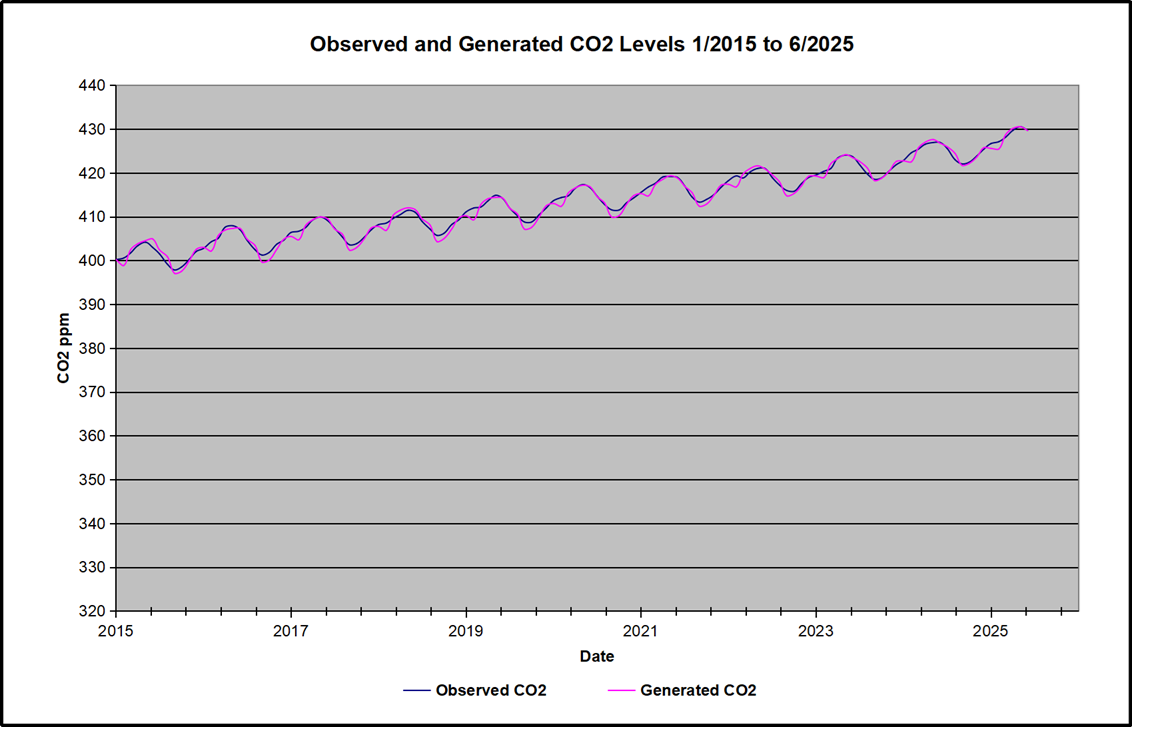
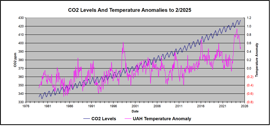
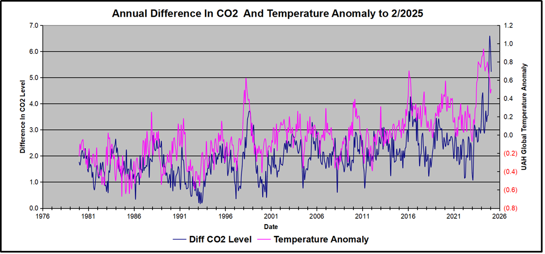
They’re shrinking because of more CO2. And the reason is that there are a number of benefits from more CO2, but one of the most important ones is that if there’s more CO2, plants can live with less water. They don’t waste as much water with more CO2 in the air, because they grow leaves with fewer holes in them so they don’t leak as much water. And the little holes, the stomata – the little mouths, that’s what it means and it’s where the CO2 comes in – don’t open as wide. So, the problem with sucking CO2 out of the air, which is what plants have to do, is for every CO2 molecule that diffuses into your leaf, you lose a hundred water molecules diffusing the other way. This is a real dilemma for the planet.

It’s true. CO2 is a greenhouse gas and it warms the Earth,
but the warming isn’t enough to matter.

It’s very small. And so, it’s probably beneficial on balance. If you double CO2, it seems like a lot, that’s a 100% increase of CO2. How much does that affect the cooling radiation that goes off to space? That sounds like a lot, but in effect it only decreases the radiation to space by 1%. So, 100% increase of CO2, 1% decrease in radiation to space. It’s a very small effect, and you don’t have to change the Earth’s temperature very much or cloudiness very much to bring it back into equilibrium with the situation before you increase the CO2.

So, it’s an ineffective climate influencer. Yet you get this demon gas that is going to cause us all to boil to death or something like that. Nothing could be further from the truth. It’s a trivial gas, but it’s very, very good for life on Earth. More CO2 has been wonderful for mankind because it helps provide the abundance of food we have today and it’s caused no harm, whatsoever.

On climate change activism having become like a religious cult

It is a religious cult for many people. Many people have stopped believing in traditional religions, you know? So, they don’t believe in God, but they need something beyond themselves to believe in. What could be more noble than saving the planet? “The planet is threatened by the demon gas CO2, so we’re going to save it.” The fact that it means essentially suicide for the human race doesn’t get into their brains. But that is what it means.

You cannot immediately eliminate CO2 and let the human population survive.
It can’t be done. So, it’s a suicide pact, you know, what is being proposed.

The movement is a joke – a little bit – but it’s not so different from a coalition of organised crime and religious fanaticism. And the religious fanatics … You know, you don’t argue with someone about their religion. This is not a joking matter. It brings crusades and religious wars and God knows what. So, that’s a big problem. There is this religious aspect; so many people now have been brainwashed into thinking there really is an emergency. And anyone who stands in the way of saving the planet is Satan incarnate. They are sincere people but they’re just badly misled.

Many of the most vociferous climate emergency folks; if you press them, they say, “Yes, the real problem is not fossil fuels, it’s human beings. You know, there are just too many people. We should not have more than a billion people.” We’re roughly eight billion now, so that means seven out of eight of us should disappear from the planet. This is extremely dangerous. It’s an evil cult.

On what has been lost owing to climate hysteria

The alarmist community recognised 20 years ago that the warming is a lot less than their models had predicted. “Just you wait,” they’d say, “Sooner or later it will warm. But in the meantime, we need something else to keep the alarm going.” And they seized on extreme weather and rising sea levels and ocean acidification… Things that really were not warming. And they changed the name from global warming to climate change because warming wasn’t going to cut it. There wasn’t enough warming.

Earth has an unstable climate which isn’t very well understood to this day, and it would be wonderful if we understood it better. But I think our ability to understand it has been set back very badly by the climate hysteria. So, what could’ve been 20, 30 years of good, basic research and real understanding of the climate has been wasted with hysteria about this false climate emergency, which does not exist. In the meantime, the real parts of the climate – which would be good to understand – have been ignored.