
Roger Andrews does a thorough job analyzing the effects of adjustments upon Surface Air Temperature (SAT) datasets. His article at Energy Matters is Adjusting Measurements to Match the Models – Part 1: Surface Air Temperatures. Excerpts of text and some images are below. The whole essay is informative and supports his conclusion:
In previous posts and comments I had said that adjustments had added only about 0.2°C of spurious warming to the global SAT record over the last 100 years or so – not enough to make much difference. But after further review it now appears that they may have added as much as 0.4°C.
For example, these graphs show warming of the GISS dataset:

Figure 2: Comparison of “Old” and “Current” GISS meteorological station surface air temperature series, annual anomalies relative to 1950-1990 means
The current GISS series shows about 0.3°C more global warming than the old version, with about 0.2°C more warming in the Northern Hemisphere and about 0.5°C more in the Southern. The added warming trends are almost exactly linear except for the downturns after 2000, which I suspect (although can’t confirm) are a result of attempts to track the global warming “pause”. How did GISS generate all this extra straight-line warming? It did it by replacing the old unadjusted records with “homogeneity-adjusted” versions.
The homogenization operators used by others have had similar impacts, with Berkeley Earth Surface Temperature (BEST) being a case in point. Figure 3, which compares warming gradients measured at 86 South American stations before and after BEST’s homogeneity adjustments (from Reference 1) visually illustrates what a warming-biased operator does at larger scales. Before homogenization 58 of the 86 stations showed overall warming, 28 showed overall cooling and the average warming trend for all stations was 0.54°C/century. After homogenization all 86 stations show warming and the average warming trend increases to 1.09°C/century:
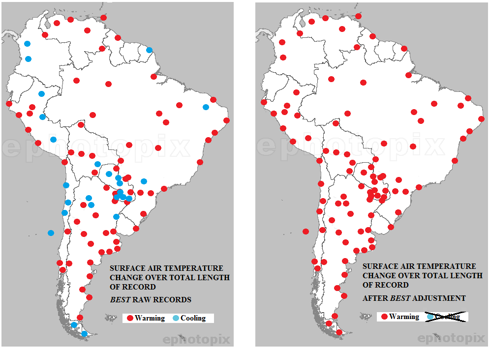
Figure 3: Warming vs. cooling at 86 South American stations before and after BEST homogeneity adjustments
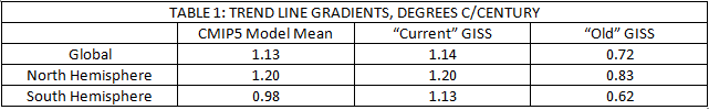
The adjusted “current” GISS series match the global and Northern Hemisphere model trend line gradients almost exactly but overstate warming relative to the models in the Southern (although this has only a minor impact on the global mean because the Southern Hemisphere has a lot less land and therefore contributes less to the global mean than does the Northern). But the unadjusted “old” GISS series, which I independently verified with my own from-scratch reconstructions, consistently show much less warming than the models, confirming that the generally good model/observation match is entirely a result of the homogeneity adjustments applied to the raw SAT records.
Summary
In this post I have chosen to combine a large number of individual examples of “data being adjusted to match it to the theory” into one single example that blankets all of the surface air temperature records. The results indicate that warming-biased homogeneity adjustments have resulted in current published series overestimating the amount by which surface air temperatures over land have warmed since 1900 by about 0.4°C (Table 1), and that global surface air temperatures have increased by only about 0.7°C over this period, not by the ~1.1°C shown by the published SAT series.
Land, however, makes up only about 30% of the Earth’s surface. The subject of the next post will be sea surface temperatures in the oceans, which cover the remaining 70%. In it I will document more examples of measurement manipulation malfeasance, but with a twist. Stay tuned.
Footnote:
I have also looked into this issue by analyzing a set of US stations considered to have the highest CRN rating. The impact of adjustments was similarly evident and in the direction of warming the trends. See Temperature Data Review Project: My Submission

Are these adjustments made to data already processed by NOAA ?
LikeLike
rw, my understanding is that NOAA applies its own homogenization algorithm to the GHCN raw data, which is different than the homogenization algorithm used by GISS, also applied to GHCN raw data. And BEST has its own adjustment process.
There is also the question of infilling missing data from other places, which is making up data, not adjusting. My own study also showed that selectively deleting records can also cause rising trends at the individual station level, even before the infilling is done.
LikeLiked by 1 person
Okay. Thanks for the clarification.
LikeLike
I spent a while looking at temperature homogenization a couple of years ago at the same time as Euan Mearns and Roger Andrews. There are two distinct methods of homogenization. The Hadley / GISS / NOAA method is the relative homogenization approach.
From Venema et al (Benchmarking homogenization algorithms for monthly data, Clim. Past, 8, 89-115, doi:10.5194/cp-8-89-2012) explain
The BEST method, I believe first derives a land-area weighted average for the temperature stations in an area. Then BEST uses “an automated procedure identifies discontinuities in the data; the data are then broken into two parts at those times, and the parts treated as separate records.”
LikeLike
It would be interesting to read what Steve Mosher would say about this.
Please submit this to WUWT.
It is important for people to start seeing the reality that like with every other apocalyptic claptrap the evidence is contrived.
LikeLike
Btw, I posted a link to this essay over at Jennifer Marohasy’s. She has been documenting data tampering in Australia for sometime, when not working on utilizing neural networking programs to research ways to do what the climate obsessed have failed to do: make better weather forecasts.
LikeLike
Where I believe all methods of temperature station homogenization break down is in the assumption (Venema et al 2012)
Having checked the data in a number of different areas (following Euan Mearns lead in many cases) this is clearly not the case. South America is a case in point. Common to eight temperature stations, covering much of southern Paraguay, was a drop in average temperatures of between 0.8 and 1.2 at the end of the 1960s. As this was not replicated in surrounding areas, so homogenization removes this feature.
LikeLike
Roger Andrews obtained a similar result independently of my own.
http://euanmearns.com/probing-the-puzzle-of-paraguayan-temperatures/
LikeLike
Thanks for adding the edifying comments manic. So, they assume a “climate signal”, then impose it on the data through adjustments. Pretty slick.
LikeLike
Had an interesting thought that maybe the skeptical science escalator graph is actually showing, pause by pause, where the actual adjustments made by Zeke and friends have been put in place.
Would it not be funny if there graph is actually proof of tampering.Will post Zekes comment when I find it which confirms all your points re adjustment.
LikeLike
Thanks angech, please do show us what Zeke had to say.
LikeLike
There is this from Dec 2014:
This comment by Zeke Hausfather:
http://www.yaleclimateconnections.org/2011/02/global-temperature-in-2010-hottest-year/
Seems to plot out the UAH and the RSS against the GISTemp and HadCRUT. They seem pretty close. Trenberth had this to say about what we may be seeing: “in terms of the global mean temperature, instead of having a gradual trend going up, maybe the way to think of it is we have a series of steps, like a staircase. And, and, it’s possible, that we’re approaching one of those steps.” Discussing a possible change to a warm PDO. The PDO by some has been described by some as confused. Not a typical cool phase but more of both phases alternating. It might be expected that a re-established cool phase would move the trend line down. This line: “And the answer is clear: the 0.116 since 1998 is not significantly different from those 0.175 °C per decade since 1979 in this sense.” By using the error bars of the 0.116, yes we can say we haven’t moved far enough away from the other number with enough confidence. The error bars for shorter time frames seem to be bigger. So the question is, has there been a relatively short term change? We are uncertain. We seem to have slowed the ascent but we can’t tell yet. If we believe in abrupt climate shifts, that would seem to place more weight on the short term point of view, in order to identify these shifts in a timely manner.
LikeLiked by 1 person
Zeke (Comment #130058)
June 7th, 2014 at 11:45 am
Mosh,
Actually, your explanation of adjusting distant past temperatures as a result of using reference stations is not correct. NCDC uses a common anomaly method, not RFM.
The reason why station values in the distant past end up getting adjusted is due to a choice by NCDC to assume that current values are the “true” values. Each month, as new station data come in, NCDC runs their pairwise homogenization algorithm which looks for non-climatic breakpoints by comparing each station to its surrounding stations. When these breakpoints are detected, they are removed. If a small step change is detected in a 100-year station record in the year 2006, for example, removing that step change will move all the values for that station prior to 2006 up or down by the amount of the breakpoint removed. As long as new data leads to new breakpoint detection, the past station temperatures will be raised or lowered by the size of the breakpoint.
An alternative approach would be to assume that the initial temperature reported by a station when it joins the network is “true”, and remove breakpoints relative to the start of the network rather than the end. It would have no effect at all on the trends over the period, of course, but it would lead to less complaining about distant past temperatures changing at the expense of more present temperatures changing.
LikeLike
Thanks angech. That explains a lot.
LikeLiked by 1 person
I would say that when a science is so self deluded that it rewrites past data then it is no longer a science but is rather a political movement.
What is clear is that human caused climate change is in fact caused by people. People who are tampering with the evidence.
LikeLike
I would love to see Zeke do the second. Cannot imagine how keeping the original temps and putting in the current temps would lead to the same trend unless one reported sll current temps as artificially high
LikeLike
If you use the unadjusted data and do the trends at the station level, you see much less warming and places that have cooled.
LikeLike
The climatocracy appears to have been “reinterpreting” the data under the guise of QC in Australia in near real time.
I wonder how much good data has been corrupted in this way worldwide?
I urge you to read and post your insights at Jennifer Marohasy’s. One argument the hypesters are using to dismiss her discovery of data tampering is that it is rare and justified.
Your work clearly shows it is worldwide.
LikeLike