Climate Science: Put Up or Shut Up

That’s the theme of an article by Rowan Dean in The Courier-Mail, Australia:  Time for climate scientists to produce evidence that carbon dioxide emissions affect climate  Full text below with my bolds and images.

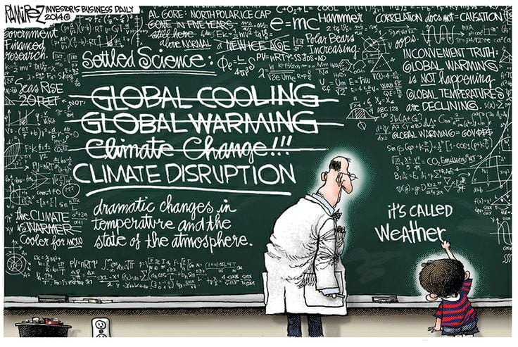
IT’S time for so-called climate scientists to either cough up one single, solitary shred of genuine scientific evidence that proves that the climate is being changed by mankind’s carbon dioxide emissions, or ‘fess up and admit that the whole thing is a gigantic hoax.

That’s the bottom line.

Asked at the beginning of this year for one of those “predictions for 2017”, I claimed that this would be the year the Australian public wakes up and realises they are being hoodwinked by the whole climate change/renewables scam.

I told Paul Murray’s lively late night TV show on Sky News that 2017 would be the year the climate con comes to an end. So how is my prediction going?

Well, so far this year two extraordinary books have come out, and one insightful film, that support my argument that the public is indeed waking up to the tricks of the climate change/renewables fraud.

Climate Change: The Facts 2017, a series of essays published by the Institute of Public Affairs, not only debunks the entire scare campaign about the Great Barrier Reef, but in a piece of superb investigative work Dr Jennifer Marohasy exposes the Bureau of Meteorology’s embarrassing manipulation of temperature data.

The book has sold out three print runs and gained serious attention overseas. Then came the surprise hit film Climate Hustle by sceptic Marc Morano, which was, ironically, more popular than the scaremongering Al Gore film it challenged.

And this week a new book is coming out by Australia’s Ian Plimer, one of our greatest geologists.

Called Climate Change Delusion and the Great Electricity Rip-off it’s a must-read for anyone who still believes they’re saving the planet by paying through the nose for electricity.  Because you’re not. The planet is doing just fine with or without your financial impoverishment, and whatever changes may or may not be occurring to our planet’s climate, it almost certainly has nothing to do with your gas bill.

As Plimer points out, Australia is blessed with an abundance of the cheapest and cleanest energy on the planet, yet we are paying the highest electricity prices on earth.

Put simply, that doesn’t add up. And when something smells fishy, it’s because it is.

Australian taxpayers are being ripped off by deluded luvvies (Turnbull is one of the worst) pandering to the voracious leeches of the renewables industry and their greedy investors gorging on a bloated smorgasbord of your cash which they siphon up via subsidies, targets and bills.

Yet, as Plimer points out, it’s all in vain. With rigorous scientific and geological data, Plimer provides evidence that the climate “experts” fail to provide. He shows that Earth has frequently warmed up, cooled down, and warmed up again, but this process has never had anything to do with CO2.

Indeed, the geological evidence is that Earth’s coldest periods often had far higher atmospheric CO2 levels than we do now. What’s more, the mild warming we may currently be experiencing (we are, geologically speaking, still in an Ice Age and moving slowly out of it) has always been associated in human history with increased health, wealth, fertility and prosperity.

Mankind’s most successful times have been in periods such as the Roman era or medieval warming when the Earth was warmer than it is now.

Indeed, we are currently seeing flora around the globe getting greener and more fertile as CO2 levels increase.

Meanwhile, desperately trying to reinvigorate the whole tiresome climate change alarmist nonsense, this year we got Al Gore’s latest horror flick-cum-ad for his own renewables investments An Inconvenient Sequel (what an unoriginal title).

Showing suitably terrifying footage of storms, floods and hurricanes, the film was a box-office flop that received lacklustre reviews at best. Oh, and the other day an ANU “climate scientist” made the hysterical (and unprovable) claim that Sydney and Melbourne “could” roast in 50 degree summers by the end of the century.

Global Mean Temperature from land and ocean expressed in absolute degrees F.

That’s it. And still no proof that man-made carbon dioxide emissions are warming the planet. Still no proof that a warmer planet can be avoided, or would actually be a bad thing. Still no proof that removing civilisation’s reliance on coal is even remotely feasible. Still no proof that even if we did do all the things climate fanatics want us to do and destroy our economies and lifestyles, it would make the slightest difference to global temperatures. And still no proof that we even need to.

The biggest con of all is that Australian voters are denied any political leadership courageous enough to call out this scaremongering for what it is, cancel all our subsidies, targets and the Paris Agreement, which only enrich renewables carpetbaggers, and return us to a land blessed with cheap, abundant energy.


A VALVE TURNER’S TRIAL: MOSTLY GUILTY October 6, 2017

Climate activist Michael Foster is on trial in North Dakota this week. The judge has barred Dr. James Hansen and other climate science experts from testifying. (Photo: Climate Direct Action)

Excerpts (my bolds) from article published in the High Plains Reader, Fargo North Dakota A Valve Turner’s Trial: Mostly Guilty

Friends call Michael Foster the valve turner a hero, the state is trying him as a criminal, and the Keystone Pipeline named him a terrorist for stopping their oil pipeline flow for eight hours in 2016.  After a week of trial and a five-hour deliberation, a jury found Foster guilty on all counts, except reckless endangerment, leaving felony criminal mischief, felony conspiracy to commit criminal mischief, and criminal trespass, a misdemeanor.

Foster’s co-defendant, Sam Jessup, who filmed the action, was convicted of felony conspiracy to commit criminal mischief and misdemeanor conspiracy trespass, both sentences which could carry a maximum of 11 years imprisonment.

Foster’s trial brought activist groups, civil rights advocates, climate change analysts, reporters from Washington D.C. and New York, to the picturesque town of Cavalier, population barely 1,300, the seat of Pembina County.

Lady Justice stands tall above the neoclassical-styled courthouse, but her scales dipped heavily with Foster’s case. On the trial’s third and fourth days, Judge Laurie A. Fontaine denied Foster’s necessity defense, denied the testimonies of four expert witnesses on Climate Change, and denied motions for acquittal by the defense.

“While the proffered experts could testify to the data supporting the existence and severity of climate change, there is no argument that they have the knowledge or expertise to testify on how knowledge of climate change affects an individual defendant’s mental state, intent, or level of culpability,” court documents said.

Foster, 52, stands accused of felonies with a maximum sentence of 22 years in prison, years more than any other activist arrested. His action – considered the biggest coordinated move on U.S. energy infrastructure undertaken by environmental protesters – has been covered by national media, but little has been reported by mainstream media in North Dakota.

Foster helped halt 15 percent of US oil consumption for the day. Jessup, who filmed Foster on October 11, 2016, is being tried as a conspirator.  Kirschner argued for his client, Jessup, that the two did not conspire; Jessup was there to film, and he never entered the manual shut-off valve control area, known as Walhalla 8-2, as it is 8.2 miles from the Canadian border.

“My client was there when a crime was being committed,” Kirschner said. “My client was there to record and live stream. Just being there doesn’t make him a conspirator to criminal trespass. There is no evidence that he said or planned anything beforehand.”

“He bragged ahead of time, he boasted after the fact,” prosecutor Byers said of Foster. “He shut down the Keystone Pipeline, he knew he would cause losses of more than $10,000. Yes, nobody was injured, but an untrained operator not knowing the equipment he’s using – it didn’t go bad, but it certainly could have. There is enough evidence to have a jury possibly convict.”

Climate guru Dr. James Hansen, a former NASA researcher, was one of the expert witnesses planning to testify. “I’m the one who said tar sands are ‘game over’ for climate, and here [is Michael Foster] facing trial for trying to do something about it.”

Sentences will be handed down next week.

Lady Justice stands tall above the neoclassical-styled courthouse, Pembina County, North Dakota

Summary

That’s three of four valve turners who failed to get the necessity defense to work.  (Minnesota case TBD)  A previous defendant, who attended this trial, got off with time served, a slap on the wrist.  This no nonsense judge seems determined to apply the law with no allowance for religious beliefs concerning the climate.  I particularly liked the ruling barring experts since it suggested that claiming climate necessity is like pleading insanity.  The sentences should be interesting.

Background on climate criminal cases: https://rclutz.wordpress.com/2017/02/04/jury-hangs-instead-of-climate-activist/


October Arctic Surprise

Click on image to enlarge.

In recent years, October has seen some rapid recoveries of Arctic ice extents.  But this year may become something special.  With the early onset of Siberian snow cover and the resulting surface cooling, ice is roaring back, especially on the Asian side.  Consider the refreezing during the last 11 days through yesterday.

The graph compares extents over the last 10 days.

2017 has reached 5.7M km2, 460k km2 more than the strong 2016 recovery, now tracking the 10 year average.  2007 remains 1.1M km2 behind, and 2012 is 1.7M km2 less than 2017.  SII is showing similar ice gains in October.

Halloween is Coming!

Footnote

Some people unhappy with the higher amounts of ice extent shown by MASIE continue to claim that Sea Ice Index is the only dataset that can be used. This is false in fact and in logic. Why should anyone accept that the highest quality picture of ice day to day has no shelf life, that one year’s charts can not be compared with another year? Researchers do this analysis, including Walt Meier in charge of Sea Ice Index. That said, I understand his interest in directing people to use his product rather than one he does not control. As I have said before:

MASIE is rigorous, reliable, serves as calibration for satellite products, and uses modern technologies to continue the long and honorable tradition of naval ice charting.  More on this at my post Support MASIE Arctic Ice Dataset


Natural Climate Factors: Snow

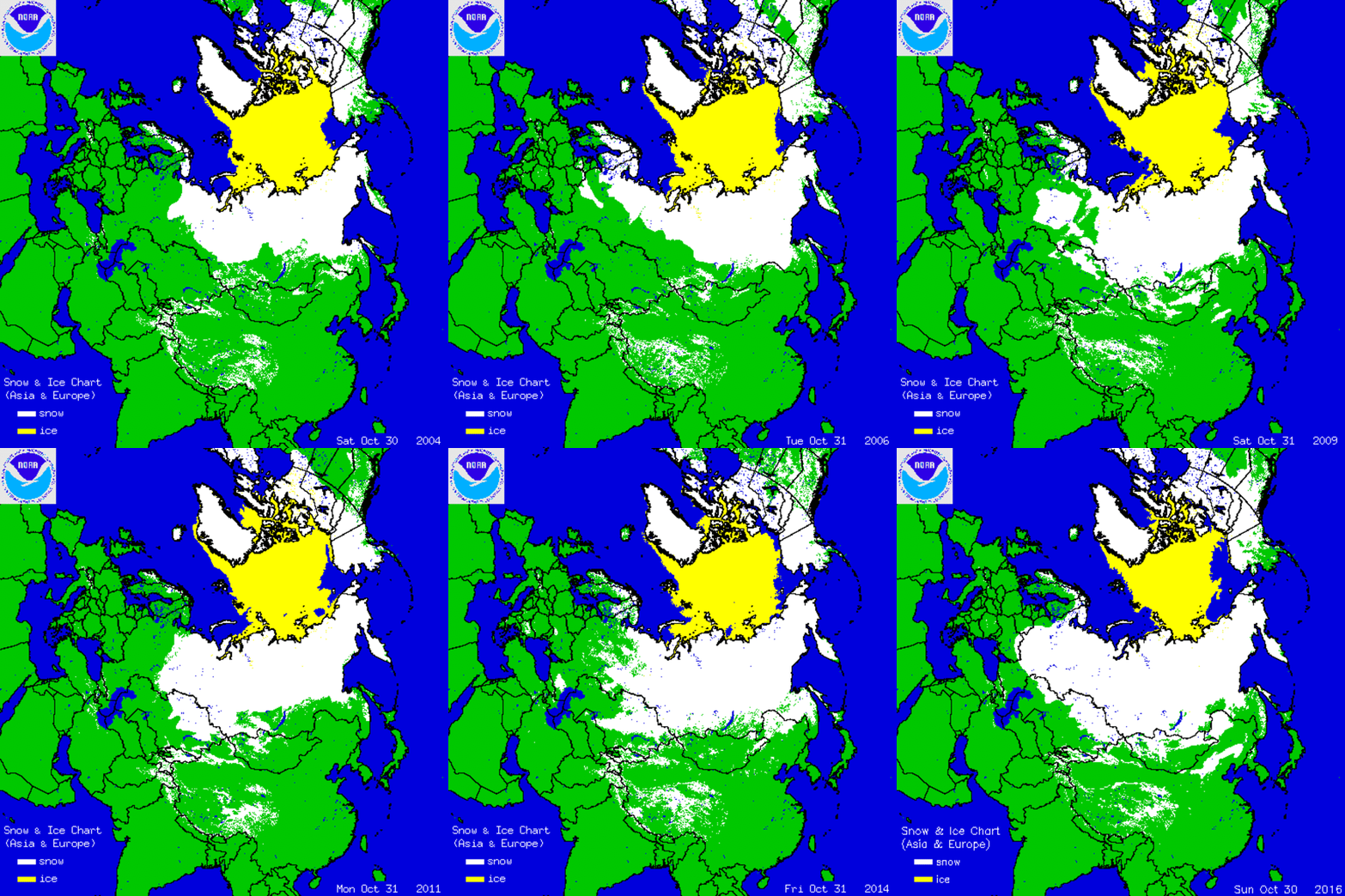
Variations in Siberian snow cover October (day 304) 2004 to 2016. Eurasian snow charts from IMS.

Previously I posted an explanation by Dr. Judah Cohen regarding a correlation between autumn Siberian snow cover and the following winter conditions, not only in the Arctic but extending across the Northern Hemisphere. More recently, in looking into Climate Model Upgraded: INMCM5, I noticed some of the scientists were also involved in confirming the importance of snow cover for climate forecasting. Since the poles function as the primary vents for global cooling, what happens in the Arctic in no way stays in the Arctic. This post explores data suggesting changes in snow cover drive some climate changes.

The Snow Cover Climate Factor

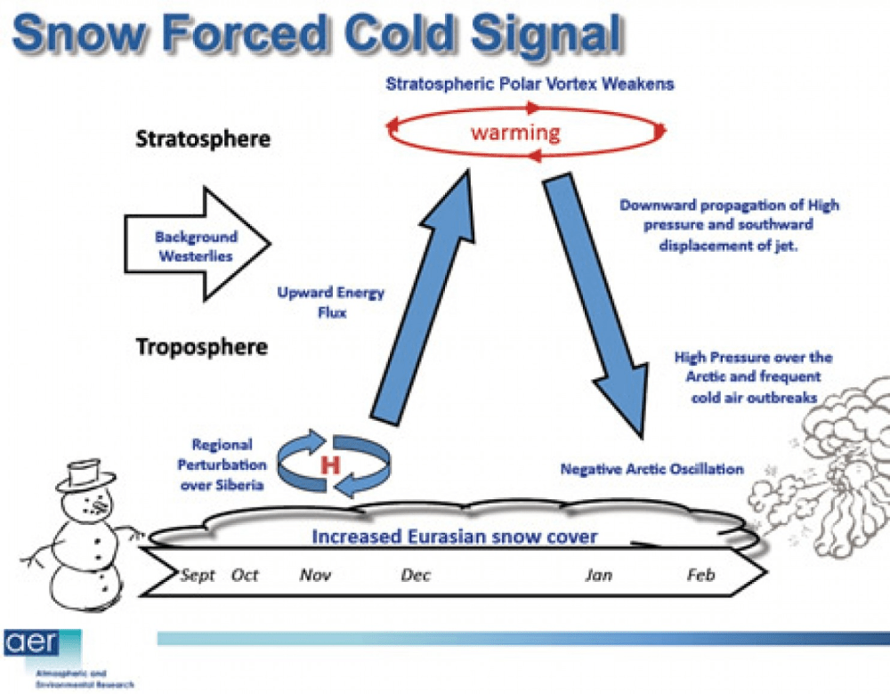
The diagram represents how Dr. judah Cohen pictures the Northern Hemisphere wintertime climate system.  He leads research regarding Arctic and NH weather patterns for AER.

cohen-schematic2

Dr. Cohen explains the mechanism in this diagram.

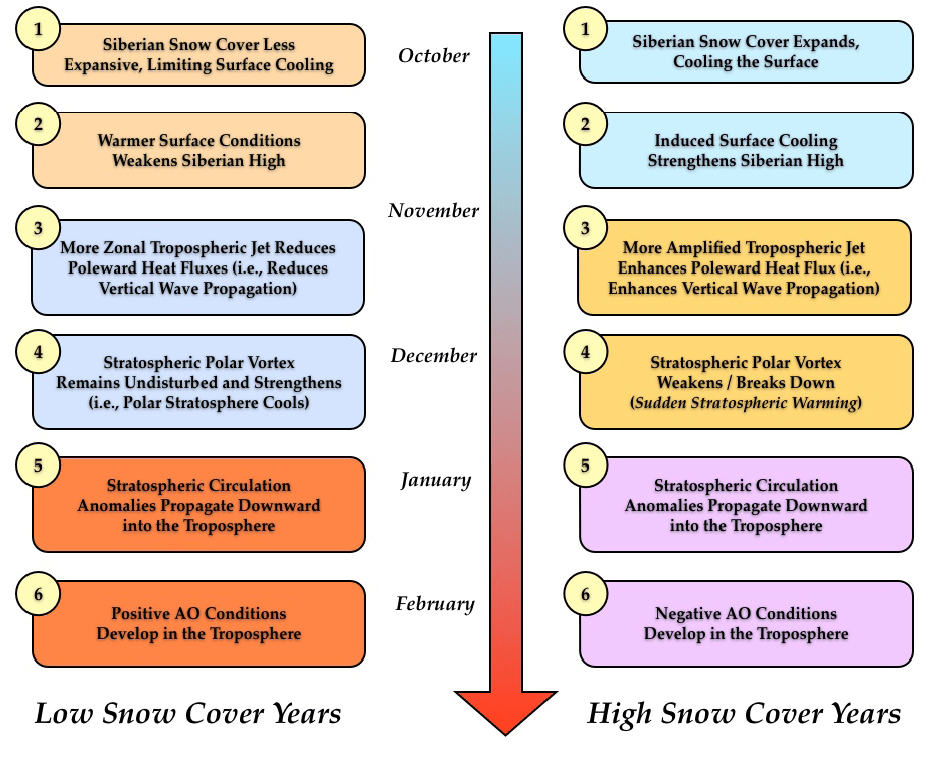
Conceptual model for how fall snow cover modifies winter circulation in both the stratosphere and the troposphere–The case for low snow cover on left; the case for extensive snow cover on right.

1. Snow cover increases rapidly in the fall across Siberia, when snow cover is above normal diabatic cooling helps to;
2. Strengthen the Siberian high and leads to below normal temperatures.
3. Snow forced diabatic cooling in proximity to high topography of Asia increases upward flux of energy in the troposphere, which is absorbed in the stratosphere.
4. Strong convergence of WAF (Wave Activity Flux) indicates higher geopotential heights.
5. A weakened polar vortex and warmer down from the stratosphere into the troposphere all the way to the surface.
6. Dynamic pathway culminates with strong negative phase of the Arctic Oscillation at the surface.

From Eurasian Snow Cover Variability and Links with Stratosphere-Troposphere
Coupling and Their Potential Use in Seasonal to Decadal Climate Predictions by Judah Cohen.

Observations of the Snow Climate Factor

The animation at the top shows from remote sensing that Eurasian snow cover fluctuates significantly from year to year, taking the end of October as a key indicator.

For several decades the IMS snow cover images have been digitized to produce a numerical database for NH snow cover, including area extents for Eurasia. The NOAA climate data record of Northern Hemisphere snow cover extent, Version 1, is archived and distributed by NCDC’s satellite Climate Data Record Program. The CDR is forward processed operationally every month, along with figures and tables made available at Rutgers University Global Snow Lab.

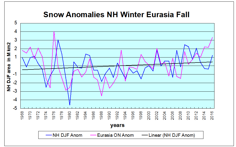
This first graph shows the snow extents of interest in Dr. Cohen’s paradigm. The Autumn snow area in Siberia is represented by the annual Eurasian averages of the months of October and November (ON). The following NH Winter is shown as the average snow area for December, January and February (DJF). Thus the year designates the December of that year plus the first two months of the next year.

Notes: NH snow cover minimum was 1981, trending upward since.  Siberian autumn snow cover was lowest in 1989, increasing since then.  Autumn Eurasian snow cover is about 1/3 of Winter NH snow area. Note also that fluctuations are sizable and correlated.

The second graph presents annual anomalies for the two series, each calculated as the deviation from the mean of its entire time series. Strikingly, the Eurasian Autumn flux is on the same scale as total NH flux, and closely aligned. While NH snow cover declined a few years prior to 2016, Eurasian snow is trending upward strongly.  If Dr. Cohen is correct, NH snowfall will follow. The linear trend is slightly positive, suggesting that fears of children never seeing snowfall have been exaggerated. The Eurasian trend line (not shown) is almost the same.

What About Winter 2017-2018?

These data confirm that Dr. Cohen and colleagues are onto something. Here are excerpts from his October 2 outlook for the upcoming season AER. (my bolds)

The main block/high pressure feature influencing Eurasian weather is currently centered over the Barents-Kara Seas and is predicted to first weaken and then strengthen over the next two weeks.

Blocking in the Barents-Kara Seas favors troughing/negative geopotential height anomalies and cool temperatures downstream over Eurasia but especially Central and East Asia. The forecast for the next two weeks across Central Asia is for continuation of overall below normal temperatures and new snowfall.

Currently the largest negative anomalies in sea ice extent are in the Chukchi and Beaufort Seas but that will change over the next month or so during the critical months of November-February. In my opinion low Arctic sea ice favors a more severe winter but not necessarily hemisphere-wide and depends on the regions of the strongest anomalies. Strong negative departures in the Barents-Kara Seas favors cold temperatures in Asia while strong negative departures near Greenland and/or the Beaufort Sea favor cold temperatures in eastern North America.

Siberian snow cover is advancing quickly relative to climatology and is on a pace similar to last year at this time. My, along with my colleagues and others, research has shown that extensive Siberian snow cover in the fall favors a trough across East Asia with a ridge to the west near the Urals. The atmospheric circulation pattern favors more active poleward heat flux, a weaker PV and cold temperatures across the NH. It is very early in the snow season but recent falls have been snowy across Siberia and therefore I do expect another upcoming snowy fall across Siberia.

Summary

In summary the three main predictors that I follow in the fall months most closely, the presence or absence of high latitude blocking, Arctic sea ice extent and Siberian snow cover extent all point towards a more severe winter across the continents of the NH.

Uh oh.  Now where did I put away my long johns?

Another Climate Push Poll

University of Chicago News headline says Most Americans want government to combat climate change, poll finds

The report is summarized in this graphic:
climate20poll202_1012

It should be obvious that for decades, opinion polls have been deployed as a marketing tool. Information is gathered, but more importantly public awareness and concern is raised according to the interests of the survey sponsors. The industry calls these “push polls” and conduct them annually, or even more frequently, intending to mold public opinion in the direction of climate alarmism, and to claim support for policies favored by sponsors.

Interpreting Poll Results

In order to take meaning from a poll, you have to know the context and specifically what questions were asked, what responses were allowed and in what sequence (i.e. the methodology).

Some contextual facts were suppressed in the above report. To discuss them, let us consider the first question put to participants:

Q31. How important are the following issues to you personally?

The grid shows results from two surveys, the last one 8/17-21/2017, and the previous one 6/8-11/2017. First column includes six issues and the number of participants in the August survey. The June survey only had five issues.  Numbers in the grid are % of responses.

8//2017 8//2017 8//2017 6//2017 6//2017 6//2017
AP-NORC/EPIC 8/17-21/2017 Not at all
/slightly
important
Moderately
important
Very/
extremely
important
Not at all
/slightly
important
Moderately
important
Very/
extremely
important
The economy (n=992) 5 18 77 4 14 81
Immigration (n=1,038) 17 32 50 21 32 47
Health care (n=992) 5 11 84 3 14 82
Climate change (n=1,038) 25 26 48 25 21 53
Terrorism (n=992) 10 22 68 8 14 77
Energy policy (n=1,038) 16 29 54 NA NA NA

Regarding Participation: We have responses from 1038 Americans, which was a completion rate of 27%. Thus these results come from a subset of people who chose to respond, and unsurprisingly they express concerns. Of course, we don’t know about what the others care.

In that context, all the issues rate as important, with climate change coming in last place in August, and next to last in June.

Regarding Survey Frame:

The Survey is entitled Public Opinion on Energy Policy under the Trump Administration, and sure enough, the second question is:
Q32. Overall, do you approve or disapprove of the way Donald Trump is handling his job as president? (with follow ups to get whether strongly or only somewhat).

Since the pollsters know more people disapprove of Trump than approve, putting this question early creates a central tendency to respond in negation to perceived Trump positions. Further, it signals that this is about politics not science.

Regarding the Survey Subject:

Now to the meat (or rather the lack of it). Next Question:
Q33. Do you think climate change is happening, do you think climate change is not happening, or aren’t you sure?

Here people are asked about an undefined buzzword “climate change” and whether it is happening or not, in their opinion. Could any question be more vacuous?
(Synonyms for “Vacuous”: silly, inane, unintelligent, insipid, foolish, stupid, fatuous, idiotic, brainless, witless, vapid, vacant, empty-headed.)

The responses tell us only about badges that people like or dislike. And since “climate change” has been a political football, used by the left as a wedge issue, this will be a positive buzzword for Democrats and a negative one for Republicans. And since the population has more Dems, and since the survey sample is 36% Democrats and 23% Republicans, the desired response is assured.

Survey Says:  Happening 72%, Not Happening 9%, Not sure 19%.

BTW in 2017 Happening is down 5% from 2016, while Not Sure is up 6%, so you can read the tea leaves any way you like.

Then, for those who think climate change is happening (Lord only knows what that actually means for any of the individuals), they then get to tell us about causation:

If climate change is happening in Q33
Q34. Do you think climate change is caused entirely by human activities, caused mostly by human activities, caused about equally by human activities and natural changes in the environment, caused mostly by natural changes in the environment, or caused entirely by natural changes in the environment?

Since this question is only put to the 72%, who said yes in Q33, the responses to Q34 are:
55% out of 774 say Caused entirely/mostly by human activities
32% out ot 774 say Caused equally by human activities and natural changes in the environment
12% out of 774 say Caused mostly/entirely by natural changes in the environment

Pollsters will be tempted to add the 32% to 55%, but that is misleading. The equally caused response is a mixed bag. Some knowledgeable people (like Dr. Curry) know that human and natural factors of global warming (if that is what we are talking about) have not yet been separated, and 50-50 can be an educated guess.

But from experience I can say that the equal causation includes many people who didn’t want to say “Don’t know.” Often these climate push polls ask people: “How much do you feel you know about global warming?” Typically about 25% say they know a lot, 60% say they know a little, and the rest less than a little. As we know from other researchers, more climate knowledge increases skepticism for many, so it is likely the soft number includes many who feel they really don’t know.

The only firm number out of this is that 41% of respondents feel that climate change is happening and that humans are mostly the cause. (426 out of 1038). Not surprisingly that finding does not appear anywhere.

Regarding Polling Bias

The poll was funded by EPIC ( Energy Policy Institute at the University of Chicago). In presenting their climate research, EPIC says this:

Climate change is considered by many to be the most urgent, global challenge. The impacts of climate change are already emerging in more damaging and frequent storms, extreme temperature changes, agricultural changes, and depleting water supplies. Efforts to address climate change, however, have proceeded slowly.

I think we can guess how EPIC personnel would answer the questionnaire.

There are many additional questions in the poll results (here)

For example, consider several questions raised regarding fracking. Included were these:

Q44B. One recent study found babies in the womb experience negative health effects from close exposure to a hydraulic fracturing site. The effects were strongest within a half mile of the site, with babies 25% more likely to have a low birth weight. Birth weights were not different for pregnant mothers living more than 2 miles from the site. Would you say you favor, oppose, or neither favor nor oppose the use of hydraulic fracturing in the United States?

Q44D. One recent study found that hydraulic fracturing triggered earthquakes in Oklahoma. The study found that the injection of wastewater, part of the hydraulic fracturing process, triggered the earthquakes. Would you say you favor, oppose, or neither favor nor oppose the use of hydraulic fracturing in the United States?

And this one tests how you feel about being an outsider.

Q40. As you may know, nearly 200 countries recently signed an international agreement in Paris to reduce greenhouse gas emissions. Do you support, oppose, or neither support nor oppose the United States withdrawing from this international agreement?

Summary

Climate change is now totally a socio-political movement in support of a $1.5 trillion industry, and the only thing that matters is winning hearts and minds (well minds maybe not). A similar survey was done in Canada, specifically to claim public support for what Trudeau wanted to do all along: Impose a carbon tax. This was done despite what that survey showed behind the smoke and mirrors.

Note that Canadians may be more picky than Americans, and so they got a question with more substance:
1. “From what you’ve read and heard, is there solid evidence that the average temperature on earth has been getting warmer over the past four decades?”
2. [If yes, solid evidence] “Is the earth getting warmer mostly because of human activity such as burning fossil fuels or mostly because of natural patterns in the earth’s environment?”
For more see Uncensored: Canadians View Global Warming

This blog has as a slogan: Reading between the lines and underneath the hype. It doesn’t look like the job is getting any lighter.  When you see or hear anything climate-related in the media, start by assuming the report is myopic, lop-sided, or both, until proven otherwise.  How to go about proving otherwise is demonstrated with several examples in the post Impaired Climate Vision.

Climate Model Upgraded: INMCM5 Under the Hood

2018 Update: Best Climate Model INMCM5 October 22, 2018 (follow link to latest info on INMCM5)

A previous analysis Temperatures According to Climate Models showed that only one of 42 CMIP5 models was close to hindcasting past temperature fluctuations. That model was INMCM4, which also projected an unalarming 1.4C warming to the end of the century, in contrast to the other models programmed for future warming five times the past.
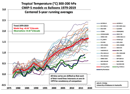
In a recent comment thread, someone asked what has been done recently with that model, given that it appears to be “best of breed.” So I went looking and this post summarizes further work to produce a new, hopefully improved version by the modelers at the Institute of Numerical Mathematics of the Russian Academy of Sciences.

Institute of Numerical Mathematics, Russian Academy of Sciences, Moscow, Russia

Earlier this year came this publication Simulation of the present-day climate with the climate model INMCM5 by E.M. Volodin et al. Excerpts below with my bolds.

In this paper we present the fifth generation of the INMCM climate model that is being developed at the Institute of Numerical Mathematics of the Russian Academy of Sciences (INMCM5). The most important changes with respect to the previous version (INMCM4) were made in the atmospheric component of the model. Its vertical resolution was increased to resolve the upper stratosphere and the lower mesosphere. A more sophisticated parameterization of condensation and cloudiness formation was introduced as well. An aerosol module was incorporated into the model. The upgraded oceanic component has a modified dynamical core optimized for better implementation on parallel computers and has two times higher resolution in both horizontal directions.

Analysis of the present-day climatology of the INMCM5 (based on the data of historical run for 1979–2005) shows moderate improvements in reproduction of basic circulation characteristics with respect to the previous version. Biases in the near-surface temperature and precipitation are slightly reduced compared with INMCM4 as  well as biases in oceanic temperature, salinity and sea surface height. The most notable improvement over INMCM4 is the capability of the new model to reproduce the equatorial stratospheric quasi-biannual oscillation and statistics of sudden stratospheric warmings.
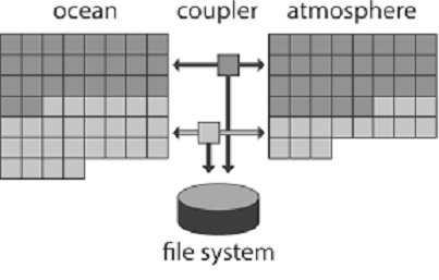
 

The family of INMCM climate models, as most climate system models, consists of two main blocks: the atmosphere general circulation model, and the ocean general circulation model. The atmospheric part is based on the standard set of hydrothermodynamic equations with hydrostatic approximation written in advective form. The model prognostic variables are wind horizontal components, temperature, specific humidity and surface pressure.

Atmosphere Module

The INMCM5 borrows most of the atmospheric parameterizations from its previous version. One of the few notable changes is the new parameterization of clouds and large-scale condensation. In the INMCM5 cloud area and cloud water are computed prognostically according to Tiedtke (1993). That includes the formation of large-scale cloudiness as well as the formation of clouds in the atmospheric boundary layer and clouds of deep convection. Decrease of cloudiness due to mixing with unsaturated environment and precipitation formation are also taken into account. Evaporation of precipitation is implemented according to Kessler (1969).

In the INMCM5 the atmospheric model is complemented by the interactive aerosol block, which is absent in the INMCM4. Concentrations of coarse and fine sea salt, coarse and fine mineral dust, SO2, sulfate aerosol, hydrophilic and hydrophobic black and organic carbon are all calculated prognostically.

Ocean Module

The oceanic module of the INMCM5 uses generalized spherical coordinates. The model “South Pole” coincides with the geographical one, while the model “North Pole” is located in Siberia beyond the ocean area to avoid numerical problems near the pole. Vertical sigma-coordinate is used. The finite-difference equations are written using the Arakawa C-grid. The differential and finite-difference equations, as well as methods of solving them can be found in Zalesny etal. (2010).

The INMCM5 uses explicit schemes for advection, while the INMCM4 used schemes based on splitting upon coordinates. Also, the iterative method for solving linear shallow water equation systems is used in the INMCM5 rather than direct method used in the INMCM4. The two previous changes were made to improve model parallel scalability. The horizontal resolution of the ocean part of the INMCM5 is 0.5 × 0.25° in longitude and latitude (compared to the INMCM4’s 1 × 0.5°).

Both the INMCM4 and the INMCM5 have 40 levels in vertical. The parallel implementation of the ocean model can be found in (Terekhov etal. 2011). The oceanic block includes vertical mixing and isopycnal diffusion parameterizations (Zalesny et al. 2010). Sea ice dynamics and thermodynamics are parameterized according to Iakovlev (2009). Assumptions of elastic-viscous-plastic rheology and single ice thickness gradation are used. The time step in the oceanic block of the INMCM5 is 15 min.
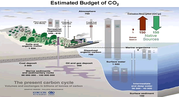
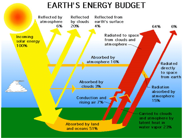
Note the size of the human emissions next to the red arrow.

Carbon Cycle Module

The climate model INMCM5 has а carbon cycle module (Volodin 2007), where atmospheric CO2 concentration, carbon in vegetation, soil and ocean are calculated. In soil, а single carbon pool is considered. In the ocean, the only prognostic variable in the carbon cycle is total inorganic carbon. Biological pump is prescribed. The model calculates methane emission from wetlands and has a simplified methane cycle (Volodin 2008). Parameterizations of some electrical phenomena, including calculation of ionospheric potential and flash intensity (Mareev and Volodin 2014), are also included in the model.

Surface Temperatures

When compared to the INMCM4 surface temperature climatology, the INMCM5 shows several improvements. Negative bias over continents is reduced mainly because of the increase in daily minimum temperature over land, which is achieved by tuning the surface flux parameterization. In addition, positive bias over southern Europe and eastern USA in summer typical for many climate models (Mueller and Seneviratne 2014) is almost absent in the INMCM5. A possible reason for this bias in many models is the shortage of soil water and suppressed evaporation leading to overestimation of the surface temperature. In the INMCM5 this problem was addressed by the increase of the minimum leaf resistance for some vegetation types.

Nevertheless, some problems migrate from one model version to the other: negative bias over most of the subtropical and tropical oceans, and positive bias over the Atlantic to the east of the USA and Canada. Root mean square (RMS) error of annual mean near surface temperature was reduced from 2.48 K in the INMCM4 to 1.85 K in the INMCM5.

Precipitation

In mid-latitudes, the positive precipitation bias over the ocean prevails in winter while negative bias occurs in summer. Compared to the INMCM4, the biases over the western Indian Ocean, Indonesia, the eastern tropical Pacific and the tropical Atlantic are reduced. A possible reason for this is the better reproduction of the tropical sea surface temperature (SST) in the INMCM5 due to the increase of the spatial resolution in the oceanic block, as well as the new condensation scheme. RMS annual mean model bias for precipitation is 1.35mm day−1 for the INMCM5 compared to 1.60mm day−1 for the INMCM4.

Cloud Radiation Forcing

Cloud radiation forcing (CRF) at the top of the atmosphere is one of the most important climate model characteristics, as errors in CRF frequently lead to an incorrect surface temperature.

In the high latitudes model errors in shortwave CRF are small. The model underestimates longwave CRF in the subtropics but overestimates it in the high latitudes. Errors in longwave CRF in the tropics tend to partially compensate errors in shortwave CRF. Both errors have positive sign near 60S leading to warm bias in the surface temperature here. As a result, we have some underestimation of the net CRF absolute value at almost all latitudes except the tropics. Additional experiments with tuned conversion of cloud water (ice) to precipitation (for upper cloudiness) showed that model bias in the net CRF could be reduced, but that the RMS bias for the surface temperature will increase in this case.
 

A table from another paper provides the climate parameters described by INMCM5.

Climate Parameters Observations INMCM3 INMCM4 INMCM5
Incoming solar radiation at TOA 341.3 [26] 341.7 341.8 341.4
Outgoing solar radiation at TOA   96–100 [26] 97.5 ± 0.1 96.2 ± 0.1 98.5 ± 0.2
Outgoing longwave radiation at TOA 236–242 [26] 240.8 ± 0.1 244.6 ± 0.1 241.6 ± 0.2
Solar radiation absorbed by surface 154–166 [26] 166.7 ± 0.2 166.7 ± 0.2 169.0 ± 0.3
Solar radiation reflected by surface     22–26 [26] 29.4 ± 0.1 30.6 ± 0.1 30.8 ± 0.1
Longwave radiation balance at surface –54 to 58 [26] –52.1 ± 0.1 –49.5 ± 0.1 –63.0 ± 0.2
Solar radiation reflected by atmosphere      74–78 [26] 68.1 ± 0.1 66.7 ± 0.1 67.8 ± 0.1
Solar radiation absorbed by atmosphere     74–91 [26] 77.4 ± 0.1 78.9 ± 0.1 81.9 ± 0.1
Direct hear flux from surface     15–25 [26] 27.6 ± 0.2 28.2 ± 0.2 18.8 ± 0.1
Latent heat flux from surface     70–85 [26] 86.3 ± 0.3 90.5 ± 0.3 86.1 ± 0.3
Cloud amount, %     64–75 [27] 64.2 ± 0.1 63.3 ± 0.1 69 ± 0.2
Solar radiation-cloud forcing at TOA         –47 [26] –42.3 ± 0.1 –40.3 ± 0.1 –40.4 ± 0.1
Longwave radiation-cloud forcing at TOA          26 [26] 22.3 ± 0.1 21.2 ± 0.1 24.6 ± 0.1
Near-surface air temperature, °С 14.0 ± 0.2 [26] 13.0 ± 0.1 13.7 ± 0.1 13.8 ± 0.1
Precipitation, mm/day 2.5–2.8 [23] 2.97 ± 0.01 3.13 ± 0.01 2.97 ± 0.01
River water inflow to the World Ocean,10^3 km^3/year 29–40 [28] 21.6 ± 0.1 31.8 ± 0.1 40.0 ± 0.3
Snow coverage in Feb., mil. Km^2 46 ± 2 [29] 37.6 ± 1.8 39.9 ± 1.5 39.4 ± 1.5
Permafrost area, mil. Km^2 10.7–22.8 [30] 8.2 ± 0.6 16.1 ± 0.4 5.0 ± 0.5
Land area prone to seasonal freezing in NH, mil. Km^2 54.4 ± 0.7 [31] 46.1 ± 1.1 48.3 ± 1.1 51.6 ± 1.0
Sea ice area in NH in March, mil. Km^2 13.9 ± 0.4 [32] 12.9 ± 0.3 14.4 ± 0.3 14.5 ± 0.3
Sea ice area in NH in Sept., mil. Km^2 5.3 ± 0.6 [32] 4.5 ± 0.5 4.5 ± 0.5 6.1 ± 0.5

Heat flux units are given in W/m^2; the other units are given with the title of corresponding parameter. Where possible, ± shows standard deviation for annual mean value.  Source: Simulation of Modern Climate with the New Version Of the INM RAS Climate Model (Bracketed numbers refer to sources for observations)

Ocean Temperature and Salinity

The model biases in potential temperature and salinity averaged over longitude with respect to WOA09 (Antonov et al. 2010) are shown in Fig.12. Positive bias in the Southern Ocean penetrates from the surface downward for up to 300 m, while negative bias in the tropics can be seen even in the 100–1000 m layer.

Nevertheless, zonal mean temperature error at any level from the surface to the bottom is small. This was not the case for the INMCM4, where one could see negative temperature bias up to 2–3 K from 1.5 km to the bottom nearly al all latitudes, and 2–3 K positive bias at levels of 700–1000 m. The reason for this improvement is the introduction of a higher background coefficient for vertical diffusion at high depth (3000 m and higher) than at intermediate depth (300–500m). Positive temperature bias at 45–65 N at all depths could probably be explained by shortcomings in the representation of deep convection [similar errors can be seen for most of the CMIP5 models (Flato etal. 2013, their Fig.9.13)].

Another feature common for many present day climate models (and for the INMCM5 as well) is negative bias in southern tropical ocean salinity from the surface to 500 m. It can be explained by overestimation of precipitation at the southern branch of the Inter Tropical Convergence zone. Meridional heat flux in the ocean (Fig.13) is not far from available estimates (Trenberth and Caron 2001). It looks similar to the one for the INMCM4, but maximum of northward transport in the Atlantic in the INMCM5 is about 0.1–0.2 × 10¹⁵ W higher than the one in the INMCM4, probably, because of the increased horizontal resolution in the oceanic block.

Sea Ice

In the Arctic, the model sea ice area is just slightly overestimated. Overestimation of the Arctic sea ice area is connected with negative bias in the surface temperature. In the same time, connection of the sea ice area error with the positive salinity bias is not evident because ice formation is almost compensated by ice melting, and the total salinity source for these pair of processes is not large. The amplitude and phase of the sea ice annual cycle are reproduced correctly by the model. In the Antarctic, sea ice area is underestimated by a factor of 1.5 in all seasons, apparently due to the positive temperature bias. Note that the correct simulation of sea ice area dynamics in both hemispheres simultaneously is a difficult task for climate modeling.

The analysis of the model time series of the SST anomalies shows that the El Niño event frequency is approximately the same in the model and data, but the model El Niños happen too regularly. Atmospheric response to the El Niño vents is also underestimated in the model by a factor of 1.5 with respect to the reanalysis data.

Conclusion

Based on the CMIP5 model INMCM4 the next version of the Institute of Numerical Mathematics RAS climate model was developed (INMCM5). The most important changes include new parameterizations of large scale condensation (cloud fraction and cloud water are now the prognostic variables), and increased vertical resolution in the atmosphere (73 vertical levels instead of 21, top model level raised from 30 to 60 km). In the oceanic block, horizontal resolution was increased by a factor of 2 in both directions.

The climate model was supplemented by the aerosol block. The model got a new parallel code with improved computational efficiency and scalability. With the new version of climate model we performed a test model run (80 years) to simulate the present-day Earth climate. The model mean state was compared with the available datasets. The structures of the surface temperature and precipitation biases in the INMCM5 are typical for the present climate models. Nevertheless, the RMS error in surface temperature, precipitation as well as zonal mean temperature and zonal wind are reduced in the INMCM5 with respect to its previous version, the INMCM4.

The model is capable of reproducing equatorial stratospheric QBO and SSWs.The model biases for the sea surface height and surface salinity are reduced in the new version as well, probably due to increasing spatial resolution in the oceanic block. Bias in ocean potential temperature at depths below 700 m in the INMCM5 is also reduced with respect to the one in the INMCM4. This is likely because of the tuning background vertical diffusion coefficient.

Model sea ice area is reproduced well enough in the Arctic, but is underestimated in the Antarctic (as a result of the overestimated surface temperature). RMS error in the surface salinity is reduced almost everywhere compared to the previous model except the Arctic (where the positive bias becomes larger). As a final remark one can conclude that the INMCM5 is substantially better in almost all aspects than its previous version and we plan to use this model as a core component for the coming CMIP6 experiment.

Summary

One the one hand, this model example shows that the intent is simple: To represent dynamically the energy balance of our planetary climate system.  On the other hand, the model description shows how many parameters are involved, and the complexity of processes interacting.  The attempt to simulate operations of the climate system is a monumental task with many outstanding challenges, and this latest version is another step in an iterative development.

Note:  Regarding the influence of rising CO2 on the energy balance.  Global warming advocates estimate a CO2 perturbation of 4 W/m^2.  In the climate parameters table above, observations of the radiation fluxes have a 2 W/m^2 error range at best, and in several cases are observed in ranges of 10 to 15 W/m^2.

We do not yet have access to the time series temperature outputs from INMCM5 to compare with observations or with other CMIP6 models.  Presumably that will happen in the future.
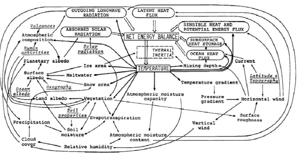
Early Schematic: Flows and Feedbacks for Climate Models
Overachieving September Arctic Ice

September daily extents are now fully reported and the 2017 September monthly results can be compared with years of the previous decade.  MASIE showed 2017 exceeded 4.8M km2  and SII was close behind, also reaching 4.8M for the month.  The 11 year linear trend is more upward for MASIE, mainly due to 2008 and 2009 reported higher in SII.  In either case, one can easily see the Arctic ice extents since 2007 have not declined and are now 500k km2 higher.

In August, 4.5M km2 was the median estimate of the September monthly average extent from the SIPN (Sea Ice Prediction Network) who use the reports from SII (Sea Ice Index), the NASA team satellite product from passive microwave sensors.

The graph below shows September comparisons through day 273 (Sept. 30).Note that starting day 260 2016 had begun its remarkable recovery, and is now well above the 10 year average, nearly matching 2017. Meanwhile 2007 is 1.1M km2 behind and the Great Arctic Cyclone year of 2012 is 1.4M km2 less than 2017.  Note also that SII is currently matching MASIE.

The narrative from activist ice watchers is along these lines:  2017 minimum is not especially low, but it is very thin.  “The Arctic is on thin ice.”  They are basing that notion on PIOMAS, a model-based estimate of ice volumes, combining extents with estimated thickness.  That technology is not mature, and in any case refers to the satellite era baseline, which began in 1979.

The formation of ice this year does not appear thin, since it is concentrated in the central Arctic.  For example, Consider how Laptev and East Siberian seas together added 180k km2 in the just the last ten days:

Click on image to enlarge.

The table shows ice extents in the regions for 2017, 10 year averages and 2007 for day 273. Decadal averages refer to 2007 through 2016 inclusive.

Region 2017273 Day 273
Average
2017-Ave. 2007273 2017-2007
 (0) Northern_Hemisphere 5200394 4944703 255690 4086883 1113511
 (1) Beaufort_Sea 397521 540936 -143415 498743 -101222
 (2) Chukchi_Sea 141983 217113 -75130 51 141932
 (3) East_Siberian_Sea 369289 326398 42891 311 368978
 (4) Laptev_Sea 377166 166604 210562 235245 141922
 (5) Kara_Sea 46667 28503 18164 15367 31300
 (6) Barents_Sea 2010 20562 -18552 4851 -2841
 (7) Greenland_Sea 134724 245771 -111046 353210 -218486
 (8) Baffin_Bay_Gulf_of_St._Lawrence 85755 48614 37141 42247 43508
 (9) Canadian_Archipelago 498801 356144 142657 307135 191666
 (10) Hudson_Bay 1621 4741 -3121 1936 -316
 (11) Central_Arctic 3143698 2988219 155479 2626511 517187

Deficits in Beaufort and Chukchi are more than offset by surpluses in East Siberian and Laptev. Kara and Barents together are average.  Greenland Sea is down but note the strong surpluses in Canadian Archipelago and the Central Arctic, which is already at 95% of its March maximum.

Summary

Earlier observations showed that Arctic ice extents were low in the 1940s, grew thereafter up to a peak in 1977, before declining.  That decline was gentle until 1994 which started a decade of multi-year ice loss through the Fram Strait.  There was also a major earthquake under the north pole in that period.  In any case, the effects and the decline ceased in 2007, 30 years after the previous peak.  Now we have a plateau in ice extents, which could be the precursor of a growing phase of the quasi-60 year Arctic ice oscillation.

For context, note that the average maximum has been 15M, so on average the extent shrinks to 30% of the March high before growing back the following winter.  In 2017 about 33% of the March maximum was retained, so the melt season losses were considerably less than in the past.

Background from Sept. 20

Dave Burton asked a great question in his previous comment, and triggered this response:

Dave, thanks for asking a great question. All queries are good, but a great one forces me to dig and learn something new, in this case a more detailed knowledge of what goes into MASIE reports.

You asked, where do they get their data? The answer is primarily from NIC’s Interactive Multisensor Snow and Ice Mapping System (IMS). From the documentation, the multiple sources feeding IMS are:

Platform(s) AQUA, DMSP, DMSP 5D-3/F17, GOES-10, GOES-11, GOES-13, GOES-9, METEOSAT, MSG, MTSAT-1R, MTSAT-2, NOAA-14, NOAA-15, NOAA-16, NOAA-17, NOAA-18, NOAA-N, RADARSAT-2, SUOMI-NPP, TERRA

Sensor(s): AMSU-A, ATMS, AVHRR, GOES I-M IMAGER, MODIS, MTSAT 1R Imager, MTSAT 2 Imager, MVIRI, SAR, SEVIRI, SSM/I, SSMIS, VIIRS

Summary: IMS Daily Northern Hemisphere Snow and Ice Analysis

The National Oceanic and Atmospheric Administration / National Environmental Satellite, Data, and Information Service (NOAA/NESDIS) has an extensive history of monitoring snow and ice coverage.Accurate monitoring of global snow/ice cover is a key component in the study of climate and global change as well as daily weather forecasting.

The Polar and Geostationary Operational Environmental Satellite programs (POES/GOES) operated by NESDIS provide invaluable visible and infrared spectral data in support of these efforts. Clear-sky imagery from both the POES and the GOES sensors show snow/ice boundaries very well; however, the visible and infrared techniques may suffer from persistent cloud cover near the snowline, making observations difficult (Ramsay, 1995). The microwave products (DMSP and AMSR-E) are unobstructed by clouds and thus can be used as another observational platform in most regions. Synthetic Aperture Radar (SAR) imagery also provides all-weather, near daily capacities to discriminate sea and lake ice. With several other derived snow/ice products of varying accuracy, such as those from NCEP and the NWS NOHRSC, it is highly desirable for analysts to be able to interactively compare and contrast the products so that a more accurate composite map can be produced.

The Satellite Analysis Branch (SAB) of NESDIS first began generating Northern Hemisphere Weekly Snow and Ice Cover analysis charts derived from the visible satellite imagery in November, 1966. The spatial and temporal resolutions of the analysis (190 km and 7 days, respectively) remained unchanged for the product’s 33-year lifespan.

As a result of increasing customer needs and expectations, it was decided that an efficient, interactive workstation application should be constructed which would enable SAB to produce snow/ice analyses at a higher resolution and on a daily basis (~25 km / 1024 x 1024 grid and once per day) using a consolidated array of new as well as existing satellite and surface imagery products. The Daily Northern Hemisphere Snow and Ice Cover chart has been produced since February, 1997 by SAB meteorologists on the IMS.

Another large resolution improvement began in early 2004, when improved technology allowed the SAB to begin creation of a daily ~4 km (6144×6144) grid. At this time, both the ~4 km and ~24 km products are available from NSIDC with a slight delay. Near real-time gridded data is available in ASCII format by request.

In March 2008, the product was migrated from SAB to the National Ice Center (NIC) of NESDIS. The production system and methodology was preserved during the migration. Improved access to DMSP, SAR, and modeled data sources is expected as a short-term from the migration, with longer term plans of twice daily production, GRIB2 output format, a Southern Hemisphere analysis, and an expanded suite of integrated snow and ice variable on horizon.

http://www.natice.noaa.gov/ims/ims_1.html

Footnote

Some people unhappy with the higher amounts of ice extent shown by MASIE continue to claim that Sea Ice Index is the only dataset that can be used. This is false in fact and in logic. Why should anyone accept that the highest quality picture of ice day to day has no shelf life, that one year’s charts can not be compared with another year? Researchers do this, including Walt Meier in charge of Sea Ice Index. That said, I understand his interest in directing people to use his product rather than one he does not control. As I have said before:

MASIE is rigorous, reliable, serves as calibration for satellite products, and continues the long and honorable tradition of naval ice charting using modern technologies. More on this at my post Support MASIE Arctic Ice Dataset