Okhotsk Shuffle Jan. 9

Click on image to enlarge.

Coinciding with the Siberian air freezing Niagara Falls and extending frigid temperatures as far south as Carolina, Arctic ice extent got quite variable in the North Pacific, especially in Okhotsk on the left.  The image above shows how ice in that basin shuffled forward, backward and forward again.

Mid-December Okhotsk Sea on the left began growing ice steadily to reach half of 2017 March max, then inexplicably lost over 300k km2 of ice in just four days. In the last nine days it more than gained back the loss.  Meanwhile, Chukchi (upper right) was frozen completely, then retreated, and now closed again.  Bering Sea on the right has been advancing steadily but more slowly than average.

Ice extents for January appear in the graph below; 2018 is shown to date, other years for the full month.  11 year average is 2007 to 2017 inclusive.

Note that 2007 catches and exceeds the 11 year average ending the month tied.  2017 and 2018 are adding ice at nearly average rate but started with deficits to average. SII 2018 has fallen further behind.

Below is the analysis of regions on day 008.  Average is for 2007 to 2017 inclusive.

Region 2018008 Day 008 
Average
2017-Ave. 2017008 2018-2017
 (0) Northern_Hemisphere 13019244 13560397 -541153 13194225 -174981
 (1) Beaufort_Sea 1070445 1070178 267 1070445 0
 (2) Chukchi_Sea 965971 966005 -34 966006 -35
 (3) East_Siberian_Sea 1087120 1087136 -16 1087137 -18
 (4) Laptev_Sea 897845 897842 3 897845 0
 (5) Kara_Sea 888549 920916 -32367 917704 -29156
 (6) Barents_Sea 343580 486463 -142883 306884 36696
 (7) Greenland_Sea 551915 599604 -47690 518372 33543
 (8) Baffin_Bay_Gulf_of_St._Lawrence 1044045 1063947 -19902 1199200 -155154
 (9) Canadian_Archipelago 853109 853040 69 853214 -106
 (10) Hudson_Bay 1260838 1241598 19240 1260887 -49
 (11) Central_Arctic 3202818 3207336 -4518 3125131 77687
 (12) Bering_Sea 212150 544302 -332152 165702 46449
 (13) Baltic_Sea 18026 42662 -24636 22885 -4859
 (14) Sea_of_Okhotsk 593649 537888 55760 783663 -190014

Note that 2018 deficit to average comes mostly from Bering and Barents Seas. The recovering ice in Okhotsk is now above average but still below last year, when Okhotsk accounts for the difference.

Background:  Updated Winter Forecast by Dr. Judah Cohen, January 8, 2018

Dr. Judah Cohen of AER published his current Arctic Oscillation and Polar Vortex Analysis and Forecast on January 8, 2018. His comments are always enlightening, and particularly so this time. Excerpts in italics with my bolds.

A minor but regionally very impactful stratospheric PV disruption promoted persistent cross polar flow that emptied Siberia of its cold air and carried it on a direct route to Southeastern Canada and the Northeastern US over the past two weeks. The historic cold of the past two weeks has placed the Eastern US in a position to finish with a cold winter but in no way, has guaranteed the outcome. I am of the opinion that for the winter in the Eastern US to finish with an overall cold solution then at least one other stratospheric PV is necessary but still may not be sufficient. Given the magnitude of the most recent cold air outbreak either a minor or major PV disruption could be enough to ensure a cold winter in aggregate over the three months from December through February.

I would argue that whether the winter will finish in the warm or cold column is science vs. art (at least my own artistic rendition). The science says that the second half of winter will be warm across the Eastern US including the remainder of January and all of February. All dynamical forecasts including most climate forecast system (CFS) forecasts, the national multi-model ensemble (NMME) and the European models all forecast warm see Figure i).

My own instinct tells me the winter will end in the cold column. Of course, the AER winter forecast predicts a cold winter based on Siberian snow cover, Arctic sea ice and tropospheric precursors. But my instinct or gut feeling is based on different metrics – the period of cold, northeastern snowfall and temperature records.

There have been some famously cold Decembers followed by a relatively mild remainder of winter. The two that most readily come to my mind are winters 1983/84 and 1989/90. One more recent but not as dramatic was winter 2005/06. And if my recollection is correct, those cold Decembers transitioned from cold to mild around the holiday season. I cannot recall a mild winter when the cold from December extended into January.

The second is significant snowfall in the I95 corridor. Again, I can’t recall a snowstorm this early in the season of the magnitude of this week’s blizzard occurring during mild winters. I certainly can’t recall any in 1983/84, 1989/90 or 2005/06, though in that last winter there was significant snowfall in February.

Finally, are record temperatures mostly in January. It seems to me that record cold or warm temperatures are an early indication of the overall winter anomaly. Record warm temperatures occur in an overall warm winters and record cold temperatures in an overall cold winter and less so vice versa. I do believe fairly strongly that Nature likes to foreshadow and those are some of the foreshadowing markers that I follow.

Interestingly below normal or convergence of vertical Wave Activity Flux (WAFz) is predicted in the troposphere for next week. This actually favors increased high latitude blocking and may explain the return of strong Alaska ridging with downstream eastern North America troughing and cold weather. But rather than a committed turn to the cold path this appears to be more of a head fake and more mild weather is predicted for the third week of January. Therefore, the return to mild weather in the Eastern US makes me believe we still remain situated at the fork in the road without a full commitment to either the mild or warm path. Though if the GFS forecast of cold reloading in Canada is correct, I think that it is almost inevitable for that cold to slide down into the lower 48 with time.

Put in other words the fork can be represented by the divergence in the polar cap geopotential heights (PCHs) between the troposphere and the stratosphere. PCHs are overall warm/positive in the troposphere while PCHs are overall cold/negative in the stratosphere. In probably overly simplistic terms I am waiting for convergence of either warm or cold PCHs throughout the troposphere and the stratosphere before claiming winter has fully committed to a cold (universal warm PCHs) or mild (universal cold PCHs) winter.

Whichever fork the ice takes, the Polar Bears had a very happy New Years Day.


Museum Offends Warmists: Tweetstorm Ensues

Correction January 9, 2018:
My terminology in the title is off.  The event is more properly called a “twitstorm.”

Wonderful example of leftist conspiracy ideation explodes when warmists are exposed to historical truth.  At the American Museum of Natural History in New York a plaque in place for 25 years has been attacked as though it were a Confederate statue. The whole story comes from a sympathetic source, the Verge:
The climate change misinformation at a top museum is not a conservative conspiracy.

The article describes a  fine dust-up of political correctness.  (Excerpts below in italics with my bolds.)

Over the weekend, Twitter users — including some climate scientists — were upset by a plaque at the American Museum of Natural History (AMNH) in New York, which seems to be spreading misinformation about climate change. The panel, titled “Recent Climatic Changes and Extinctions,” misstates the role that human emissions of greenhouse gases play in causing global warming. It also says that, although we’re currently living in one of Earth’s warm periods, “there is no reason to believe that another Ice Age won’t come.” But it turns out, the panel was put up 25 years ago, according to the museum, so it contains outdated information that reads very differently today.

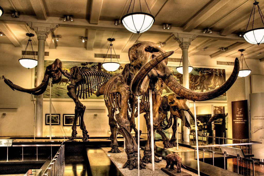
From an exhibit on Recent Climatic Changes and Extinctions:

The Offensive Text on the Plaque

Images of the sign were first tweeted by environmental economist Jonah Busch, and were shared over 2,000 times. Busch tweeted that the panel is at the David H. Koch Dinosaur Wing, which was funded by right-wing philanthropist and fossil fuel magnate David H. Koch, and asked the museum to “separate this panel from its donor’s interest.” The tweet sparked outrage among scientists and the general public: “Dear @AMNH I bring my young kids to visit regularly because science & natural history is fascinating, inspiring and fun,” one tweet read. “Please do not misguide their curious minds. If we can’t even trust the AMNH to give us the facts who can we? Very sad.”

But the sign is actually located in the Hall of Advanced Mammals in the Lila Acheson Wallace Wing of Mammals and Their Extinct Relatives, and was installed “many years before David Koch supported the Dinosaur Halls,” says Kendra Snyder, a spokesperson for the AMNH, in an email to The Verge. Busch says he didn’t realize that hall was separate from the dinosaur wing because both are on the same floor. Because some of the permanent exhibitions at the AMNH were funded by Exxon as well as the Koch brothers, which are known funders of climate deniers, “it makes it that much harder to give them the benefit of the doubt,” Busch tells The Verge. But Snyder says that at the AMNH, “scientific and educational content is determined by scientists and educators. That is not the role of donors.”

The sign reflects the scientific data available at the time, Snyder says, adding that today, that same information is “clearly subject to misinterpretation.” “If that label copy were written today it would likely come with a different context and emphasis, including more recent scientific data,” Snyder says. “This happens sometimes in permanent halls and we do review existing content — this is a case where we will do that.”

The journalist adds her spin to the story:
The dinosaur wing at the AMNH still bears his name. But the plaque in question is not in that wing, according to Snyder. The sign explains what causes ice ages, Earth’s cyclical periods when temperatures drop and glaciers spread. The sign says that, “There is no reason to believe that another Ice Age won’t come. In the past, warm cycles lasted about 10,000 years, and it’s been that long since the last cool period.” But that’s probably wrong, based on what we know today. Because we pump heat-trapping greenhouse gases like carbon dioxide into the atmosphere, the world is warming up — and that is messing up Earth’s cycles of cold and warm spells. In fact, our CO2 emissions will delay the onset of the next ice age by at least 100,000 years.

The sign in the dinosaur wing also says that, “Human-made pollutants may also have an effect on the Earth’s climatic cycle.” Today, using the word “may” is misleading: the role our greenhouse gas emissions play in causing climate change is well established. Virtually all scientists agree that human activities, such as the burning of fossil fuels, are to blame for the warming up of our planet. In fact, the entire world — except the United States — is working together to cut emissions in order to curb global warming.

Summary

Such a tragedy that a supposedly safe space like a museum would mention cooling in the future. Our CO2 emissions prohibit anything but a warmer future.  Human CO2 ensures that the next ice age is postponed almost indefinitely, and that should be on a big sign that everyone can see. And wishy-washy words like “may” have no place in the world as warmists know it.

Can anything in the building be trusted?  Everyone be vigilant! (sarc/off)

Will Lawyers Destroy Science?

Justice: Blind and scientifically illiterate. (Credit: Storyblocks)

Several posts on this blog report on legal maneuvers as anti-fossil fuel activists turn to the courts to advance their agenda.  Now we have an article questioning whether legal thinking is relevant to scientific issues.  From Alex Berezow, editor of RealClearScience: (Full text below in italics with my bolds)

Will Lawyers Destroy Science?

Scientists and lawyers do not get along. There’s a reason for that. Simply put, scientists and lawyers do not think alike.

I was smacked in the face by this reality when I was called into jury duty in 2011. The case involved a car accident, and the standard in Washington State for the jury to decide in favor of the plaintiff is a “preponderance of evidence,” which is a fancy way of saying, “51 percent.” Essentially, a coin toss decides if the plaintiff wins a bunch of money.

The judge asked if any of the potential jurors objected to that. I did. “I’m a scientist,” I explained, “and I need more evidence than that.” So, I was shown the door.*

That experience taught me that scientists and lawyers live in two completely different worlds. Scientists want 95% confidence and margins of error; lawyers want 51% confidence. Scientists want all evidence to be considered; lawyers do everything in their power to dismiss evidence they don’t like. Scientists rely on reports written by experts; lawyers often consider them inadmissible hearsay. At their best, scientists pursue truth; at their best, lawyers pursue the truth, so long as it benefits the client.

These are fundamentally irreconcilable worldviews that are forever destined to be in conflict. And the lawyers are winning.

Scales of justice Alaska Commons

Will Lawyers Destroy Science?

Consider Mark Jacobson, the climate scientist who is suing a prestigious journal for $10 million because it hurt his feelings. There is good reason to believe that the lawsuit will be dismissed, but not before lawyers have collected a nice fee for themselves. Jacobson’s attorneys and the journal’s attorneys can both make a lot of money arguing with each other, even if the suit never actually goes to trial. Routinely, lawyers are required to solve problems that they themselves created. If something like this were to occur in any other area of life, it would be called racketeering.

Recently, RealClearScience wrote an article that covered a paper published in the journal Case Reports in Gastrointestinal Medicine about how a particular herbal tea was linked to acute liver failure. The maker of the tea threatened to sue RealClearScience, which pulled the article because it didn’t want to deal with a lawyer.

In both examples, the scientific enterprise is collateral damage. The mere threat of a lawsuit can be used to shut down scientific debate. This is deeply troubling.

A Lawsuit-Happy Nation

Unfortunately, there are no signs of such lawsuit abuse stopping. Researchers at Harvard’s John M. Olin Center for Law, Economics, and Business published a report that showed that the number of lawsuits filed in the United States far exceeds those of similar countries:

On a per capita basis, the lawsuit rate in the U.S. is higher than Canada (by 4 times), Australia (3.8x), Japan (3.3x), France (2.4x), and the UK (1.6x).

Beware, science. A lawsuit-happy nation turns its eyes to you.

*Note: Mission accomplished. I didn’t want to be there, anyway.

Dr. Alex Berezow is the Founding Editor of RealClearScience and Assistant Editor of RealClearWorld. He also is a member of the USA Today Board of Contributors. Furthermore, he co-authored the book Science Left Behind, which sold more than 5,000 copies. His work regularly appears in USA Today and The Economist, among other publications. In 2010, he earned a Ph.D. in microbiology from the University of Washington.

See Also:

Critical Climate Intelligence for Jurists (and others)

Climate Scientist Sues Over Hurt Feelings


Arctic Ice Mixed Signals

Click on image to enlarge.

With 2017 ice extent estimates complete we can look at the year in perspective.  Above is a graph showing the annual average extents since 2007, comparing MASIE and SII (v3.0).  Obviously, the trend in MASIE could not be flatter, while SII shows a decline.  The first five years the two indices were nearly the same, and since then SII shows less ice, about 260k km2 each year.  Note also how small is the variance year over year: Standard deviation is +/- 260k km2, or about 2.5% of the average annual extent.  This holds for both indices.  Note also a pattern of three higher years followed by two lower years.

A previous post Sea Ice Index Updates to v.3.0 reported on the newest SII version, and we can see how it compares with MASIE over this last year.

Click on image to enlarge.

The first four months show more diversity, both in the 10 year averages and in 2017 results. From May on MASIE 2017 tracks closely to its average, while SII shows 2017 below its average every month. For those who want to see the numbers a table is provided below.

Units 2007
to 2016
2017 2007
to 2016
2017
M km2 MASIE MASIE SII SII
Jan 13.921 13.503 13.686 13.174
Feb 14.841 14.478 14.553 14.112
Mar 15.053 14.509 14.815 14.273
Apr 14.353 13.941 14.206 13.760
May 12.763 12.838 12.757 12.618
June 10.906 10.975 10.938 10.720
July 8.359 8.383 8.107 7.901
Aug 5.955 6.006 5.657 5.472
Sept 4.663 4.832 4.676 4.797
Oct 6.630 6.804 6.734 6.715
Nov 9.897 9.697 9.718 9.458
Dec 12.235 11.972 12.063 11.752
Annual Ave. 10.798  10.661  10.659  10.396 

Some are proclaiming dire warnings about melting ice and imagining various dangerous impacts. Some fluctuations do appear but not very large and somewhat cyclical. Since 2007 it resembles a plateau more than anything else.

Background on MASIE Data Sources

MASIE reports are generated by National Ice Center from the Interactive Multisensor Snow and Ice Mapping System (IMS). From the documentation, the multiple sources feeding IMS are:

Platform(s) AQUA, DMSP, DMSP 5D-3/F17, GOES-10, GOES-11, GOES-13, GOES-9, METEOSAT, MSG, MTSAT-1R, MTSAT-2, NOAA-14, NOAA-15, NOAA-16, NOAA-17, NOAA-18, NOAA-N, RADARSAT-2, SUOMI-NPP, TERRA

Sensor(s): AMSU-A, ATMS, AVHRR, GOES I-M IMAGER, MODIS, MTSAT 1R Imager, MTSAT 2 Imager, MVIRI, SAR, SEVIRI, SSM/I, SSMIS, VIIRS

Summary: IMS Daily Northern Hemisphere Snow and Ice Analysis

The National Oceanic and Atmospheric Administration / National Environmental Satellite, Data, and Information Service (NOAA/NESDIS) has an extensive history of monitoring snow and ice coverage.Accurate monitoring of global snow/ice cover is a key component in the study of climate and global change as well as daily weather forecasting.

The Polar and Geostationary Operational Environmental Satellite programs (POES/GOES) operated by NESDIS provide invaluable visible and infrared spectral data in support of these efforts. Clear-sky imagery from both the POES and the GOES sensors show snow/ice boundaries very well; however, the visible and infrared techniques may suffer from persistent cloud cover near the snowline, making observations difficult (Ramsay, 1995). The microwave products (DMSP and AMSR-E) are unobstructed by clouds and thus can be used as another observational platform in most regions. Synthetic Aperture Radar (SAR) imagery also provides all-weather, near daily capacities to discriminate sea and lake ice. With several other derived snow/ice products of varying accuracy, such as those from NCEP and the NWS NOHRSC, it is highly desirable for analysts to be able to interactively compare and contrast the products so that a more accurate composite map can be produced.

The Satellite Analysis Branch (SAB) of NESDIS first began generating Northern Hemisphere Weekly Snow and Ice Cover analysis charts derived from the visible satellite imagery in November, 1966. The spatial and temporal resolutions of the analysis (190 km and 7 days, respectively) remained unchanged for the product’s 33-year lifespan.

As a result of increasing customer needs and expectations, it was decided that an efficient, interactive workstation application should be constructed which would enable SAB to produce snow/ice analyses at a higher resolution and on a daily basis (~25 km / 1024 x 1024 grid and once per day) using a consolidated array of new as well as existing satellite and surface imagery products. The Daily Northern Hemisphere Snow and Ice Cover chart has been produced since February, 1997 by SAB meteorologists on the IMS.

Another large resolution improvement began in early 2004, when improved technology allowed the SAB to begin creation of a daily ~4 km (6144×6144) grid. At this time, both the ~4 km and ~24 km products are available from NSIDC with a slight delay. Near real-time gridded data is available in ASCII format by request.

In March 2008, the product was migrated from SAB to the National Ice Center (NIC) of NESDIS. The production system and methodology was preserved during the migration. Improved access to DMSP, SAR, and modeled data sources is expected as a short-term from the migration, with longer term plans of twice daily production, GRIB2 output format, a Southern Hemisphere analysis, and an expanded suite of integrated snow and ice variable on horizon.

http://www.natice.noaa.gov/ims/ims_1.html

Footnote

Some people unhappy with the higher amounts of ice extent shown by MASIE continue to claim that Sea Ice Index is the only dataset that can be used. This is false in fact and in logic. Why should anyone accept that the highest quality picture of ice day to day has no shelf life, that one year’s charts can not be compared with another year? Researchers do this, including Walt Meier in charge of Sea Ice Index. That said, I understand his interest in directing people to use his product rather than one he does not control. As I have said before:

MASIE is rigorous, reliable, serves as calibration for satellite products, and continues the long and honorable tradition of naval ice charting using modern technologies. More on this at my post Support MASIE Arctic Ice Dataset

Arctic Year End: Okhotsk Surprise.

Arctic ice extent grows slowly this time of year since many regions are already covered completely.  In recent days 2017 reached 84% of the maximum last March, but dropped below the 10 year average.  As we can see, most of the action was a dramatic seesaw in Okhotsk Sea, a Siberian basin in the North Pacific.

Mid-December Okhotsk Sea on the left began growing ice steadily to reach half of 2017 March max, then inexplicably lost over 300k km2 of ice in just four days.  Meanwhile, Chukchi (upper right) froze completely, then retreated somewhat.  Bering Sea on the right has been advancing steadily but more slowly than average.

The overall effect in December is shown in the graph below:
Note that 2007 matches the 10 year average, while 2012 is well above.  Lagging behind are 2016, 2017 and SII 2017.  This year’s deficit to average appears in the last 11 days, mostly due to Bering and the Okhotsk year end surprise.
Most of the month combined Bering and Okhotsk (B&O) extents were average, until the inexplicable drop starting day 361. Except for those two seas, the month was unremarkable.
At year end, 2017 NH ice, excluding B&O, is down about 200k km2, or 2% of average.  Below is the analysis of regions on day 365.

Region 2017365 Day 365
Average
2017-Ave. 2007364 2017-2007
 (0) Northern_Hemisphere 12628187 13148939 -520752 13049737 -421550
 (1) Beaufort_Sea 1070445 1070225 220 1069711 734
 (2) Chukchi_Sea 943883 966001 -22118 965971 -22089
 (3) East_Siberian_Sea 1087120 1087134 -14 1087120 0
 (4) Laptev_Sea 897845 897841 4 897845 0
 (5) Kara_Sea 892689 888842 3848 871851 20839
 (6) Barents_Sea 331819 448769 -116950 334577 -2758
 (7) Greenland_Sea 555757 584649 -28892 666135 -110378
 (8) Baffin_Bay_Gulf_of_St._Lawrence 978074 1025197 -47123 1074827 -96753
 (9) Canadian_Archipelago 853109 853054 55 852556 553
 (10) Hudson_Bay 1260838 1227587 33251 1260856 -19
 (11) Central_Arctic 3191526 3207659 -16133 3199726 -8200
 (12) Bering_Sea 194350 446066 -251716 373942 -179592
 (13) Baltic_Sea 13345 34329 -20984 9972 3374
 (14) Sea_of_Okhotsk 336595 387522 -50928 371241 -34646

Most of 2017 deficit is in Bering and Barents, less so in Okhotsk with yesterday’s recovery.  Perhaps the Polar Vortex sent frigid air into the US and Canada and replaced it with warmer southern air, and ice receded as a result.  I have reported on Arctic incursions in a post Arctic Inversions and Intrusions but the speed of the effect on ice (if that is the phenomenon) is still surprising.  We shall see if it persists or not.

Background:  Winter Forecast by Dr. Judah Cohen, Dec. 25

On Christmas Day Dr. Judah Cohen published his updated Arctic Oscillation and Polar Vortex Analysis and Forecast  Excerpts below

As I have been discussing the past two blog posts I continue to believe that this is the most critical period of the winter and will ultimately determine the character of the winter. In my opinion, we have approached a fork in the road and the atmosphere can take two possible paths one is a path where the rest of the winter is relatively mild across the mid-latitudes of the NH and the second is a colder path or solution. The tropospheric polar vortex has been relatively weak for much of the month of December as illustrated by the relatively warm polar cap geopotential heights (PCHs) for the first half of December that then boomeranged off the mid-stratosphere and after a short respite with colder tropospheric PCHs, warmer PCHs in the troposphere are predicted through the end of the month and into early January.

Based on the easterly phase of the Quasi-Biennial Oscillation (QBO) I have been favoring a significant PV disruption most likely in January for much of the fall.  A significant stratospheric PV disruption would then be followed by an extended period of severe winter weather across the mid-latitudes of the NH.  However, I have to admit as of yet there are no signs of this scenario.  There is still time but not much.  However, there is another scenario that could still yield a relatively cold winter and that is one analogous to what happened in the winter of 2013/14 where no significant disruptions of the stratospheric occurred but rather repeated minor disruptions that yielded a cold winter for central and eastern North America. Though at first, I acknowledged this possibility I was hesitant to favor this scenario.  However, the longer the delay in a major disruption of the stratospheric PV the more I favor this scenario.

The Arctic Oscillation (AO) is currently slightly positive and is predicted to trend slowly negative through the end of the week towards neutral. The forecast is for the AO to remain close to neutral next week, likely a sign of uncertainty.

Figure 7. Forecasted snowfall anomalies (mm/day; shading) from 31 December 2017 – 4 January 2018. The forecasts are from the 00Z 18 December 2017 GFS ensemble. Note the new projection to provide finer resolution.

The current positive AO is reflective of mixed pressure/geopotential height anomalies across the Arctic and mostly positive pressure/geopotential height anomalies across the mid-latitudes. The North Atlantic Oscillation (NAO) is also currently slightly positive with weak pressure/geopotential height anomalies across Greenland and Iceland and positive pressure/geopotential height anomalies across the mid-latitudes of the North Atlantic.

A return to Ural ridging/blocking at the turn of the calendar year favors active energy transfer from the troposphere to the stratosphere. Another pulse is predicted to commence this week and peak the first few days of January. The pulse itself is likely related to relaxation of the pattern and mild temperatures across North America. However, the predicted resultant perturbation to the stratospheric polar vortex (PV) especially the building of heights over northwestern North America in my opinion could once again favor the return of cold temperatures across eastern North America later in January.

Figure 9. Forecasted snowfall anomalies (mm/day; shading) from 5 – 9 January 2018. The forecasts are from the 00Z 25 December 2017 GFS ensemble. Troughing and/or cold temperatures will support the potential of additional snowfall across Eastern Europe, Siberia, West and East Asia, Alaska, Canada and the Northwestern US. Despite below normal temperatures, temperatures warm sufficiently to support snowmelt across the Eastern US (Figure 9).

Ice did not grow this past week on the North Pacific side of the Arctic basin, still I expect the negative ice anomalies in the region to shrink.  Sea ice is below normal in the Barents-Kara Seas as well and with time the greatest negative sea ice anomalies will likely reside in this region.  As I have been writing for much of the fall I do believe that the record low sea ice anomalies in the Chukchi and Bering Seas has focused ridging/blocking in this region.  Though model forecasts do not predict a return of the blocking in the foreseeable future.

Recent research has shown that regional anomalies are important and the sea ice region most highly correlated with the winter AO is the Barents-Kara Seas region where low Arctic sea ice favors a negative winter AO and a cold Eurasia.  Below normal sea ice in this region may be contributing to more active Wave Activity Flux/poleward heat transport predicted in the models that eventually could result in a negative AO.

As we have seen, the Polar Vortex did indeed return to North America, freezing Niagara Falls in the process.

Whichever fork the ice takes, the Polar Bears had a Merry Christmas