Latest INM Climate Model Projections Triggered by Scenario Inputs

The latest climate simulation from the Russian INM was published in April 2024: Simulation of climate changes in Northern Eurasia by two versions of the INM RAS Earth system model. The paper includes discussing how results are driven greatly by processing of cloud factors.  But first for context readers should be also aware of influences from scenario premises serving as model input, in this case  SSP3-7.0.

Background on CIMP Scenario  SSP3-7.0

A recent paper reveals peculiarities with this scenario.  Recognizing distinctiveness of SSP3-7.0 for use in impact assessments by Shiogama et al (2024).  Excerpts in italics with my bolds and added images.

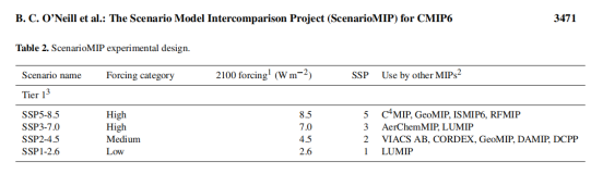
Because recent mitigation efforts have made the upper-end scenario of the future GHG concentration (SSP5-8.5) highly unlikely, SSP3-7.0 has received attention as an alternative high-end scenario for impacts, adaptation, and vulnerability (IAV) studies. However, the ‘distinctiveness’ of SSP3-7.0 may not be well-recognized by the IAV community. When the integrated assessment model (IAM) community developed the SSP-RCPs, they did not anticipate the limelight on SSP3-7.0 for IAV studies because SSP3-7.0 was the ‘distinctive’ scenario regarding to aerosol emissions (and land-use land cover changes). Aerosol emissions increase or change little in SSP3-7.0 due to the assumption of a lenient air quality policy, while they decrease in the other SSP-RCPs of CMIP6 and all the RCPs of CMIP5. This distinctive high-aerosol-emission design of SSP3-7.0 was intended to enable climate model (CM) researchers to investigate influences of extreme aerosol emissions on climate.

SSP3-7.0 Prescribes High Radiative Forcing

SSP3-7.0 Presumes High Aerosol Emissions

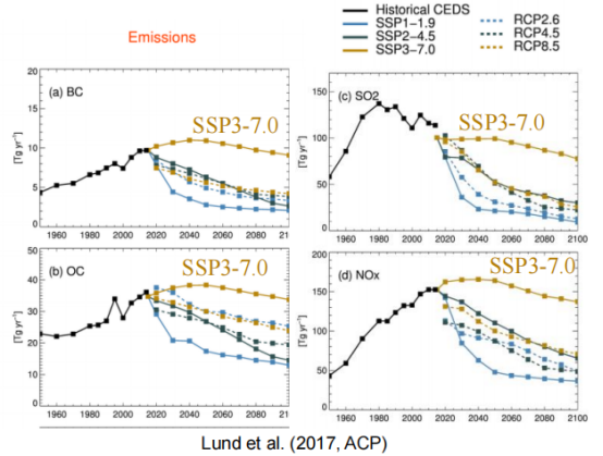
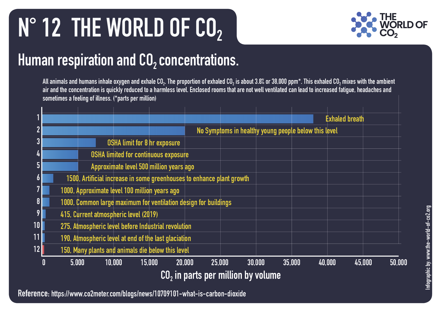
Aerosol Emissions refer to Black Carbon, Organic Carbon, SO2 and NOx.

•  Aerosol emissions increase or change little in SSP3-7.0 due to the assumption of a lenient air quality policy, while they decrease in the other SSP-RCPs of CMIP6 and all the RCPs of CMIP5.

• This distinctive high-aerosol-emission design of SSP3- 7.0 was intended to enable AerChemMIP to investigate the consequences of continued high levels of aerosol emissions on climate.

SSP3-7.0 Supposes Forestry Deprivation

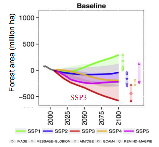
• Decreases in forest area were also substantial in SSP3- 7.0, unlike in the other SSP-RCPs.
• This design enables LUMIP to analyse the climate influences of extreme land-use and land-cover changes.

SSP3-7.0 Projects High Population Growth in Poorer Nations

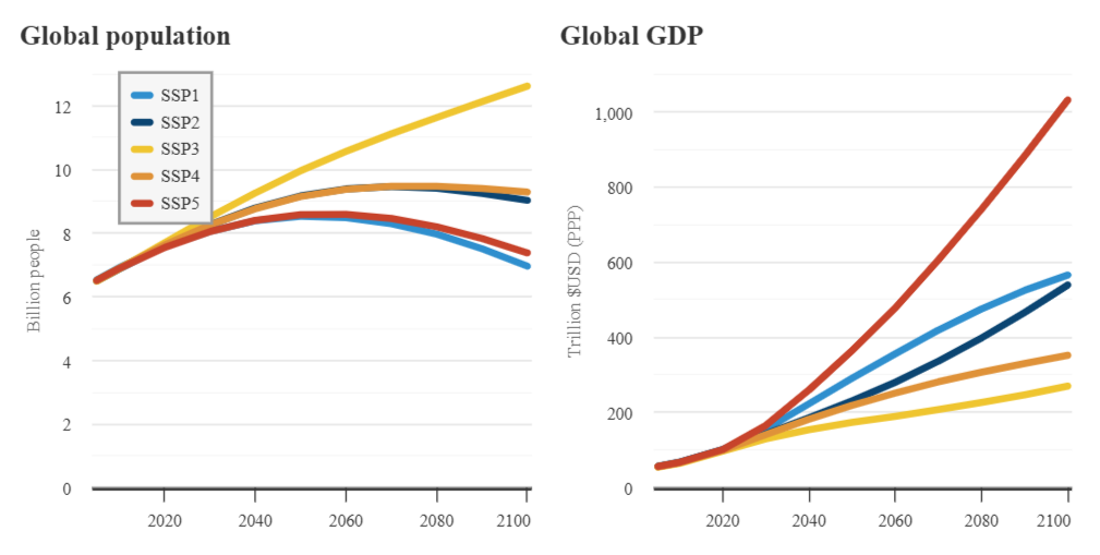
Global population (left) in billions and global gross domestic product (right) in trillion US dollars on a purchasing power parity (PPP) basis. Data from the SSP database; chart by Carbon Brief using Highcharts.

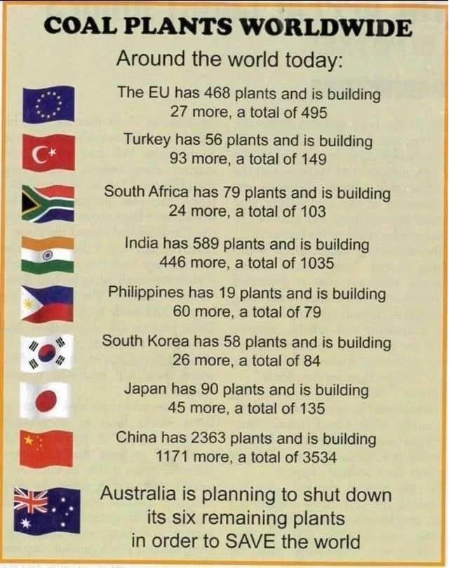
SSP3-7.0 Projects Growing Use of Coal Replacing Gas and Some Nuclear

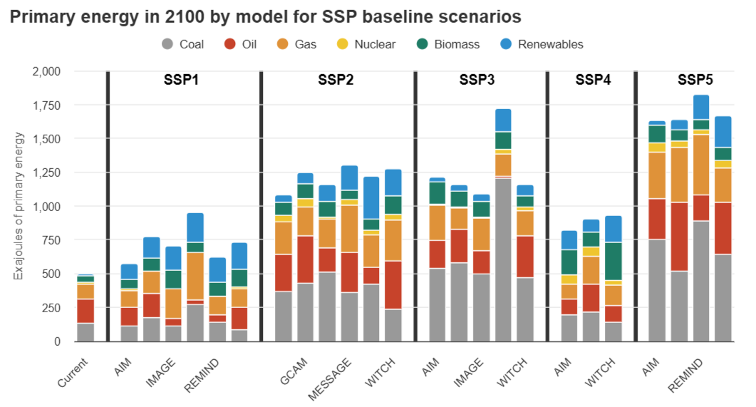
My Summary:  Using this scenario presumes high CO2 Forcing (Wm2), high aerosol emissions and diminished forest area, as well as much greater population and coal consumption. Despite claims to the contrary, this is not a “middle of the road” scenario, and a strange choice for simulating future climate metrics due to wildly improbable assumptions.

How Two Versions of a Reasonable INM Climate Model Respond to SSP3-7.0

The preceding information regarding the input scenario provides a context for understanding the output projections from INMCM5 and INMCM6.  Simulation of climate changes in Northern Eurasia by two versions of the INM RAS Earth system model. Excerpts in italics with my bolds and added images.

Introduction

The aim of this paper is the evaluation of climate changes during last several decades in the Northern Eurasia, densely populated region with the unprecedentedly rapid climate changes, using the INM RAS climate models. The novelty of this work lies in the comparison of model climate changes based on two versions of the same model INMCM5 and INMCM6, which differ in climate sensitivities ECS and TCR, with data from available observations and reanalyses. By excluding other factors that influence climate reproduction, such as different cores of GCM components, major discrepancies in description of physical process or numerical schemes, the assessment of ECS and TCR role in climate reproduction can be the exclusive focus. Also future climate projections for the middle and the end of 21st century in both model versions are given and compared.

After modification of physical parameterisations, in the model version INMCM6 ECS increased from 1.8K to 3.7K (Volodin, 2023), and TCR increased from 1.3K to 2.2K. Simulation of present-day climate by INMCM6 Earth system model is discussed in Volodin (2023). A notable increase in ECS and TCR is likely to cause a discrepancy in the simulation of climate changes during last decades and the simulation of future climate projections for the middle and the end of 21st century made by INMCM5 and INMCM6.

About 20% of the Earth’s land surface and 60% of the terrestrial land cover north of 40N refer to Northern Eurasia (Groisman et al, 2009). The Hoegh-Guldberg et al (2018) states that the topography and climate of the Eurasian region are varied, encompassing a sharply continental climate with distinct summer and winter seasons, the northern, frigid Arctic environment and the alpine climate on Scandinavia’s west coast. The Atlantic Ocean and the jet stream affect the climate of western Eurasia, whilst the Mediterranean region, with its hot summers, warm winters, and often dry spells, influences the climate of the southwest. Due to its location, the Eurasian region is vulnerable to a variety of climate-related natural disasters, including heatwaves, droughts, riverine floods, windstorms, and large-scale wildfires.

Historical Runs

One of the most important basic model experiments conducted within the CMIP project in order to control the model large-scale trends is piControl (Eyring et al, 2016). With 1850 as the reference year, PiControl experiment (Eyring et al, 2016) is conducted in conditions chosen to be typical of the period prior to the onset of large-scale industrialization. Perturbed state of the INMCM model at the end of the piControl is taken as the initial condition for historical runs. The historical experiment is conducted in the context of changing external natural and anthropogenic forcings. Prescribed time series include:

♦  greenhouse gases concentration,
♦  the solar spectrum and total solar irradiance,
♦  concentrations of volcanic sulfate aerosol in the stratosphere, and
♦  anthropogenic emissions of SO2, black, and organic carbon.

The ensemble of historical experiments consists of 10 members for each model version. The duration of each run is 165 model years from 1850 to 2014.

SSP3-7.0 Scenario

Experiments are designed to simulate possible future pathways of climate evolution based on assumptions about human developments including: population, education, urbanization, gross domestic product (GDP), economic growth, rate of technological developments, greenhouse gas (GHG) and aerosol emissions, energy supply and demand, land-use changes, etc. (Riahi et al, 2016). Shared Socio-economic Pathways or “SSP” vary from very ambitious mitigation and increasing shift toward sustainable practices (SSP1) to fossil-fueled development (SSP5) (O’Neill et al, 2016).

Here we discuss climate changes for scenario SSP3-7.0 only, to avoid presentation large amount of information. The SSP3-7.0 scenario reflects the assumption on the high GHG emissions scenario and priority of regional security, leading to societies that are highly vulnerable to climate change, combined with relatively high forcing level (7.0 W/m2 in 2100). On this path, by the end of the century, average temperatures have risen by 3.0–5.5◦C above preindustrial values (Tebaldi et al, 2021). The ensembles of historical runs with INMCM5 and INMCM6 were prolonged for 2015-2100 using scenario SSP3-7.0.

Observational data and data processing

Model near surface temperature and specific humidity changes were compared with ERA5 reanalysis data (Hersbach et al, 2020), precipitation data were compared with data of GPCP (Adler et al, 2018), sea ice extent and volume data were compared with satellite obesrvational data NSIDC (Walsh et al, 2019) and the Pan-Arctic Ice Ocean Modeling and Assimilation System (PIOMAS) (Schweiger et al, 2011) respectively, land snow area was compared with National Oceanic and Atmospheric Administration Climate Data Record (NOAA CDR) of Snow Cover Extent (SCE) reanalysis (Robinson et al, 2012) based on the satellite observational dataset Estilow et al (2015). Following Khan et al (2024) Northern Eurasia is defined as land area lying within boundaries of 35N–75N, 20E–180E. Following IPCC 6th Assessment Report (Masson-Delmotte et al, 2021), the following time horizons are distinguished: the recent past (1995– 2014), near term (2021–2040), mid-term (2041–2060), and long term (2081–2100). To compare observed and model temperature and specific humidity changes in the recent past, data for years 1991–2020 were compared with data for years 1961–1990.

Near surface air temperature change

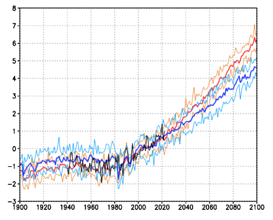
Fig. 1 Annual near surface air temperature change in Northern Eurasia with respect to 1995–2014 for INMCM6 (red), INMCM5 (blue) and ERA5 reanalysis (Hersbach et al, 2020)(black), K. Orange and lightblue lines show ensemble spread.

Despite different ECS, both model versions show (Fig. 1) approximately the same warming over Northern Eurasia by 2010–2015, similar to observations. However, projections of Northern Eurasia temperature after year 2040 differ. By 2100, the difference in 2-m air temperature anomalies between two model versions reaches around 1.5 K. The greater value around 6.0 K is achieved by a model with higher sensitivity. This is consistent with Huusko et al (2021); Grose et al (2018); Forster et al (2013), which confirmed that future projections show a stronger relationship than historical ones between warming and climate sensitivity. In contrast to feedback strength, which is more important in forecasting future temperature change, historical warming is more associated with model forcing. Both INMCM5 and INMCM6 show distinct seasonal warming patterns. Poleward of about 55N the seasonal warming is more pronounced in winter than in summer (Fig. 2). That means the smaller amplitude of the seasonal temperature cycle in 1991– 2020 compared to 1961–1990. The same result was shown in Dwyer et al (2012) and Donohoe and Battisti (2013). The opposite situation is observed during the hemispheric summer, where stronger warming is observed over the Mediterranean region (Seager et al, 2014; Kr¨oner et al, 2017; Brogli et al, 2019), subtropics and midlatitudinal regions of the Pacific Ocean, leading to an amplification of the seasonal cycle. The spatial patterns of projected warming in winter and summer in model historical experiments for 1991-2020 relative to 1961-1990 are in a good agreement with ERA5 reanalysis data, although for ERA5 the absolute values of difference are greater.

East Atlantic/West Russia (EAWR) Index

The East Atlantic/West Russia (EAWR) pattern is one of the most prominent large-scale modes of climate variability, with centers of action on the Caspian Sea, North Sea, and northeast China. The EOF-analysis identifies the EAWR pattern as the tripole with different signs of pressure (or 500 hPa geopotential height) anomalies encompassing the aforementioned region.

In this study, East Atlantic/ West Russia (EAWR) index was calculated as the projection coefficient of monthly 500 hPa geopotential height anomalies to the second EOF of monthly reanalysis 500 hPa geopotential height anomalies over the region 20N–80N, 60W–140E.

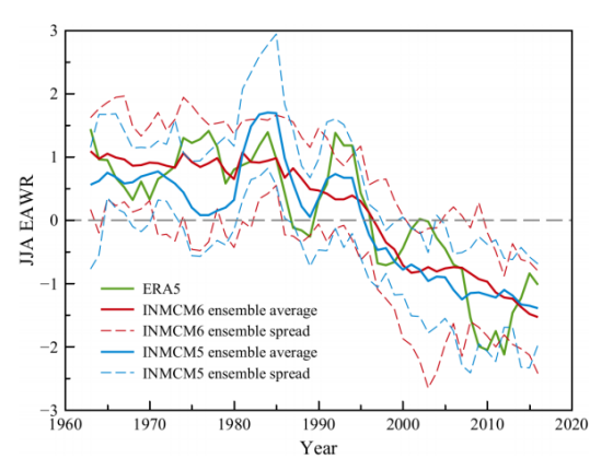
Fig. 5 Time series of June-July-August 5-year mean East Atlantic/ West Russia (EAWR) index. Maximum and minimum of the model ensemble are shown as a dashed lines. INMCM6 and INMCM5 ensemble averaged indices are plotted as a red and blue solid lines, respectively.  The ERA5 (Hersbach et al, 2020) EAWR index is shown in green.

[Note: High EAWR index indicates low pressure and cooler over Western Russia, high pressure and warmer over Europe. Low EAWR index is the opposite–high pressure and warming over Western Russia, low pressure and cooling over Europe.]

East Atlantic/ West Russia (EAWR) index Time series of EAWR index can be seen in Fig. 5. Since the middle of 1990s the sign of EAWR index has changed from positive to negative according to reanalysis data. Both versions of the INMCM reproduce the change in the sign of EAWR index. Therefore, the corresponding climate change in the Mediterranean and West Russia regions should be expected. Actually, the difference in annual mean near-surface temperature and specific humidity between 2001–2020 and 1961–1990 shows warmer and wetter conditions spreading from the Eastern Mediterranean to European Russia both for INMCM6 and INMCM5 with the largest difference being observed for the new version of model.

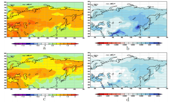
Fig. 6 Annual mean near surface temperature, K (left) and specific humidity, kg/kg (right) in 2001– 2020 with respect to 1961–1990 for INMCM6 (a,b) and INMCM5 (c,d).

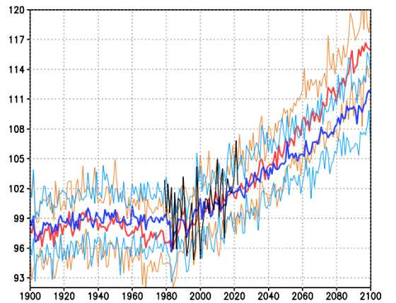
Fig. 7 Annual precipitation change (% with respect to 1995–2014) in Northern Eurasia for INMCM6 (red), INMCM5 (blue) and GPCP analysis (Adler et al, 2018) (black). Orange and lightblue lines show ensemble spread.

Discussion and conclusions

Climate changes during the last several decades and possible climate changes until 2100 over Northern Eurasia simulated with climate models INMCM5 and INMCM6 are considered. Two model versions differ in parametrisations of cloudiness, aerosol scheme, land snow cover and atmospheric boundary layer, isopycnal diffusion discretisation and dissipation scheme of the horizontal components of velocity. These modifications in atmosphere and ocean blocks of the model have led to increase of ECS to 3.7 K and TCR to 2.2 K, mainly due to modification of cloudiness parameterisation.

Comparison of model data with available observations and reanalysis show that both models simulate observed recent temperature and precipitation changes consistently with observational datasets. The decrement of seasonal temperature cycle amplitude poleward of about 55N and its increase over the Mediterranean region, subtropics, and mid-latitudinal Pacific Ocean regions are two distinct seasonal warming patterns that are displayed by both INMCM5 and INMCM6. In the long-term perspective, the amplification of difference in projected warming during June-JulyAugust (JJA) and December-January-February (DJF) increases. Both versions of the INMCM reproduce the observed change in the sign of EAWR index from positive to negative in the middle of 1990s, that allows to expect correct reproduction of the corresponding climate change in the Mediterranean and West Russia regions.

Specifically, the enhanced precipitation in the North Eurasian region since the mid-1990s has led to increased specific humidity over the Eastern Mediterranean and European Russia, which is simulated by the INMCM5 and INMCM6 models. Both versions of model correctly reproduce the precipitation change and continue its increasing trend onwards.

Both model versions simulate similar temperature, precipitation, Arctic sea ice extent in 1990–2040 in spite of INMCM5 having much smaller ECS and TCR than INMCM6. However, INMCM5 and INMCM6 show differences in the long-term perspective reproduction of climate changes. After 2040, model INMCM6 simulated stronger warming, stronger precipitation change, stronger Arctic sea ice and land snow extent decrease than INMCM5.

My Comment

So both versions of the model replicate well the observed history.  And when fed the SSP3-7.0 inputs, both project a warmer, wetter world out to 2100; INMCM5 reaches 4.5C and INMCM6 gets to 6.0C.  The scenario achieves the desired high warming, and the cloud enhancements in version 6 amplify it.  I would like to see a similar experiment done with the actual medium scenario SSP2-4.5.

Signs of Sun Setting on Renewables

News come from renewables trailblazing Australia including signs there and around the world that wind and solar power are losing their momentum. From the Australian by way of John Ray is the article The sun is setting the renewables ‘superpower’ fantasy of the Australian Left. Excerpts in italics with my bolds and added images.

Renewable energy superpower status is supposedly in Australia’s grasp now the government has given Mike Cannon-Brookes the green light to export solar power to Singapore.

Sky News Business Editor Ross Greenwood says Australia’s largest solar farm to date has been given the “green light” by the Environment Minister Tanya Plibersek.  Plibersek announced environmental approval for the tech billionaire’s eccentric proposal last week, taking a swipe at Peter Dutton’s “expensive nuclear fantasy that may never happen”.

By contrast, the Environment Minister would have us believe Cannon-Brookes’s plan to siliconise the NT Outback is a done deal. All that’s left to do is:

♦  raise $35bn in capital,
♦  install 120 square kilometres of solar panels,
♦  build a modest 788km transmission line to Darwin, and
♦  lay a 4200km high-voltage cable on the seabed, and we’re good to go.

The Sun Cable AAPowerLink project feels like it was stolen from a Heath Robinson cartoon: a convoluted, unnecessarily elaborate, and impractical contraption designed to accomplish a mundane task. It may mark the beginning of the end of the renewable romance, the point at which the transition to wind, solar and hydropower collapses under the weight of its own absurdity.

There is increasing evidence the US has reached the point of peak renewables, as the pool of private investors shrinks and winning community approval becomes harder. Research by the Lawrence Berkley National Laboratory showed roughly one-third of utility-scale wind and solar applications submitted over the past five years were cancelled, while about half of wind and solar projects experienced significant delays.

The US Department of Energy says the national electricity network needs to grow by 57 per cent by 2035, the equivalent of approximately 21,000 km a year. Last year’s total was around 200 km, downfrom just over 1000 in 2022.

Meanwhile, the challenges of grid synchronisation and storage remain unresolved, and the technical problems for offshore wind turbines, in particular, are mounting. Last week, turbine manufacturer GE Vernova announced an investigation into a blade failure in the 3.6GW Dogger Bank project in the North Sea off the coast of the UK. It is the third blade failure this year.

In July, a newly installed blade crumbled at the Vineyard Wind offshore plant, creating debris that washed up on Nantucket Island, Massachusetts. At 107 metres long and weighing 55 tonnes, they are the most enormous blades deployed commercially. The failure of three in quick succession suggests the quest to increase output by installing ever-larger blades has reached its natural limits.

Yet the imperative of expanding generating capacity is hardening.

The principal driving force is not electric vehicles but the rapid growth of artificial intelligence. AI requires at least 10 times the power of conventional computing programs.

In the US, data centres account for about 2.5 per cent of power and demand could rise to 7.5 per cent by 2030, according to Boston Consulting Group. In Ireland, data processing and storage use 12 per cent of electricity produced, forcing the authorities to limit the number of connections to the grid.

Silicon Valley has long abandoned the notion it can be powered by silicon photovoltaic panels while burying stray emissions in the Amazon forests.

In April, the tech giant Amazon paid the best part of $1bn ($US650m) for a sizeable block of land next to Pennsylvania’s Susquehanna nuclear power station. It will be the site for a data centre powered by up to 480MW of carbon-free electricity delivered reliably around the clocky.

Shares in US nuclear power companies such as Consolidated Energy, Talem and Vistra have soared by between 80 per cent and 180 per cent in the past year. So-called green energy stocks, on the other hand, are static or falling, while coal is making an unexpected comeback.

In May, the Financial Times reported that the retirement dates for coal-fired power stations are being pushed back as operators become concerned about grid security. Allianz Energy has delayed the conversion of its Wisconsin plant from coal to gas for three years to 2028. Ohio-based FirstEnergy announced in February that it was scrapping its 2030 target to phase out coal, citing “resource adequacy concerns”.

The effect of AI on electricity demand was largely unanticipated at the beginning of the decade. AI chips will undoubtedly become more efficient, but there is no telling how much further the demand for AI will grow since the technology is in its infancy. Nor can we begin to guess what other power-hungry forms of technology might be developed by 2050.

What we do know, however, is that if Australia’s demand for electricity exceeds 313 TWH a year in a 2050, we’re in trouble. That’s the target the Australian Energy Market Operator has set in its updated blueprint for the great electricity transition.

As Chris Bowen points out, that’s going to take a lot solar panels and wind turbines. The Energy Minister says we need 22,000 new solar panels a day and a new 7MW wind turbine every 18 hours just to meet our 2030 target of a mere 202 TWH. For the record, the speed of the rollout in the first two years of Labor government is less than a tenth of that.

One of the hallmarks of the anointed is an unwavering conviction
in the integrity of their analysis and
the effectiveness of their proposed solutions.

They feel no need to hedge their bets by factoring in contingency arrangements should their predictions turn out to be wrong. Nothing in AEMO’s Integrated System Plan indicates its experts have given any thought to scaling up electricity production in line with actual demand, which may well be considerably higher than they’ve anticipated.

If they had, they would have to acknowledge that there are limits to the renewable energy frontier determined by energy density, the demand for land and the requirement for firming. The silicification of northern Australia cannot continue forever, nor can we expect to rely on China for most of the hardware and pretend there are no geopolitical consequences.

As for our nuclear-phobic Prime Minister’s dream of turning Australia into the Saudi Arabia of green hydrogen, while simultaneously sitting at the cutting edge of quantum computing, forget it. In 2006, as the shadow minister for the environment, Anthony Albanese gave a speech at the Swansea RSL on avoiding dangerous climate change.

Why on Earth would we want to take the big health and economic risk of nuclear energy when we have a ready-made power source hovering peacefully in the sky every day?” he asked.

If Albanese doesn’t know the answer to that question 18 years later, he probably never will.

Being Properly Skeptical of Expert Consensus

Solvay conference 1927, probably the most intelligence ever photographed. 17 of the 29 attendees were or became Nobel Prize winners.

Miriam Solomon writes at  iai news Scientific consensus needs dissent.  Excerpts in italics with my bolds and added images

We place high epistemic value on expert opinion and when it reaches a consensus, we may view this as settled science. But, writes Miriam Solomon, we should not equate expert opinion with certainty. While expertise is a valuable guide to decision-making, experts can be prone to human error too. Laypeople can, and should, critically evaluate how expert consensus is reached.

We live in an immense, complex world, and frequently benefit from guidance from those with more information and experience—people we regard as experts—to make sense of it. Along these lines, we often use expert consensus as an indicator of what is known, and expert disagreement as an indicator of what is uncertain. So, for example, earth scientist and historian Naomi Oreskes appeals to the record of peer-reviewed scientific publications on climate change to argue that the public should listen to the expert consensus that there is anthropogenic climate change. Oreskes identified that those who publicly disagree with this consensus have not contributed to the peer-reviewed scientific literature on climate science, and in this way they are not experts with regard to the relevant subject matter, although they may have PhDs and even university positions in unrelated sciences. [Note that position ignores many expert climatologists who disagree, but who are dismissed as “deniers” because they dissent.]

Survey starting the narrative “97% consensus of experts agree humans are causing global warming.”

Oreskes dissuades us from taking such non-expert disagreement seriously, especially since she also finds that it is politically motivated. The appeal to expertise encourages us to trust those who know more than we do about a particular matter and invites us to pay attention to reliable markers of expertise, such as publication in relevant peer-refereed journals. In traditional epistemological terms, it recommends deference to epistemic authority (or authorities).

However, even experts are fallible. Expert consensus
should not be equated with certainty or truth.

But experts are more likely to be correct than non-experts, and the agreement of experts with one another can provide additional evidence for the robustness of their conclusions.  Oreskes’ approach implicitly relies on the trustability of the relevant experts, not only on their expertise. We need to know not only that experts are knowledgeable but that they are acting in the best interests of furthering knowledge. The integrity of science—its commitment to norms such as openness of inquiry, responsiveness to criticism, disinterestedness, etc. (see Merton (1942) and Longino (1990))—is vital for its trustability.

Sometimes, this trust can be eroded. Philosopher of medicine Maya Goldenberg has explored what is needed for laypersons to build justified trust in vaccine research, mentioning concerns about Big Pharma producing biased research and concerns about the historical record of medical, scientific, and governmental communities’ willingness to use untested medical technologies on marginalized groups.

When experts disagree—a common occurrence in science—deference to expertise yields conflicting results. Laypersons are apt to respond to such disagreements, such as which sorts of diets are best for long-term health, or which vaccines should be mandated and for whom, with statements such as “even the experts don’t know.”

Knowing this, experts are aware of the need for a public
face of consensus on matters they wish to influence
.

They have become savvy about disseminating any publicly relevant consensus that is achieved. This thinking is behind established institutions such as the United States’ NIH Consensus Development Conference Program (1977-2013), which issued regular reports on new clinical interventions, and the Intergovernmental Panel on Climate Change (1988-present), which issues regular updates on climate science.

Forcing a consensus when the science is not there rarely works.

Deferring to the consensus of trustable experts is one of the best kinds of argument based on epistemic authority. It is certainly better than the Scholastic practice of referring to the writings of just one “great man,” such as Aristotle or Aquinas. Several experts coming to the same conclusion about a matter is usually more convincing than one expert coming to that conclusion. However, as many have pointed out, the strength of the argument depends on:

(1) the degree of independence of these experts from each other, and
(2) the individual and collective interests of these experts.

Scientists, like the rest of us, come to their knowledge in social context and, generally speaking, scientists are neither independent of each other nor completely interest-free. They are often trained similarly—by the same schools, people, and educational materials—and feel pressured towards group conformity as well as towards deference to uber-experts. Scientists have individual biases, such as confirmation bias, that can be magnified when one scientist influences another. There are many well-known cases in the history of science and medicine in which expert consensus has turned out to be incorrect and harmful. Some examples in medicine are the traditional practice of blood-letting as a general cure-all, the use of surgery and antacids for stomach ulcers, and the practice of radical mastectomy for early stage breast cancer.

Thus, while deferring to the consensus of experts is often a good practice, it is defeasible: there are circumstances in which that deference is not ultimately justified. It is worth spelling out what those circumstances are. Here are some questions to ask of any purported expert consensus.

♦  Who agrees? Is there any dissent—if so, is it between particular groups of experts (say, family medicine practitioners disagreeing with radiologists about the effectiveness of screening mammography) or between experts and non-experts?

♦  What do the dissenters say? It is necessary to get at least a little “into the weeds” of dissent to decide whether or not dissenters are worth taking seriously.

♦  How long has there been agreement? If agreement is new, what brought it about? In particular, how much of a role did new evidence play?

♦  If agreement is longstanding, would counterevidence be sought, noticed and responded to?


These kinds of questions are a check on the processes that led to consensus. There will always be some social processes such as peer pressure and graduate school training that are unrelated to relevant evidence yet play a role in expert belief formation. This does not mean that we should distrust all consensus that has any sources in “bias.” That is too idealistic. Instead, we should look at the complete picture of what played a role in consensus formation and try to assess whether new evidence had a deciding role.

It is also worth reflecting that consensus is not the general end goal of science. Scientific communities tolerate—even benefit from—lack of consensus. Already in the nineteenth century, the philosopher John Stuart Mill put things especially well in On Liberty (1859) when he argued that consensus is an obstacle to progress, rationality and truth because it eliminates points of view that may turn out to be partially or wholly correct, or at least useful for criticism and consequent refinement of the correct view.

Dissent is strategically valuable when it leads to the distribution of cognitive labour over a variety of perspectives, hypotheses, and methods. While individual experts are often over-confident about their own views, this does little harm when it does not get in the way of other experts exploring alternatives. It is best to have the scientific community pursue all promising lines of inquiry.

Achieving consensus on a scientific matter becomes important only when there is a need for cooperative communal action and there needs to be agreement on steps to take to achieve a policy goal, such as health or sustainability. Even in such cases, there need not be agreement on all issues. The publications of the Intergovernmental Panel on Climate Change are quite clear that there is plenty of disagreement between scientists on some of the details of climate science. What is emphasized is that there is sufficient consensus on basic matters to guide important policy decisions. 

Expert consensus is an important, but not infallible, guide for laypeople and decision-makers. The strength of a consensus depends on the independence of the experts involved and the processes that shaped their agreement. While deference to experts is often justified, it should be accompanied by critical scrutiny, particularly when consensus is used to guide public policy. Dissent within the scientific community remains essential, not only for advancing knowledge but also for ensuring that consensus, when achieved, is robust and reliable.


Climate Policies Fail in Fact and in Theory

A recent international analysis of 1500 climate policies around the world concluded that 63 or 4% of them were successful in reducing emissions.  The paper is Climate policies that achieved major emission reductions: Global evidence from two decades published at Science.org.  Excerpts in italics with my bolds.

Abstract

Meeting the Paris Agreement’s climate targets necessitates better knowledge about which climate policies work in reducing emissions at the necessary scale. We provide a global, systematic ex post evaluation to identify policy combinations that have led to large emission reductions out of 1500 climate policies implemented between 1998 and 2022 across 41 countries from six continents. Our approachintegrates a comprehensive climate policy database with a machine learning–based extension ofthe common difference-in-differences approach. We identified 63 successful policy interventions with total emission reductions between 0.6 billion and 1.8 billion metric tonnes CO2 . Our insights on effective but rarely studied policy combinations highlight the important role of price-based instruments in well-designed policy mixes and the policy efforts necessary for closing the emissions gap.

Context

(1). Although the [Paris] agreement seeks to limit global average temperature increase to “well below 2°C above pre-industrial levels and pursuing efforts to limit the temperature increase to 1.5°C,” its success critically hinges on the implementation of effective climate policies at the national level.  However, scenarios from global integrated assessment models suggest that the aggregated mitigation efforts communicated through nationally determined contributions (NDCs) fall short of the required emission reductions.

(2)The United Nations (UN) estimates quantify a median emission gap of 23 billion metric tonnes(Gt) carbon dioxide equivalent (CO2-eq) by 2030

(3). The persistence of this emissions gap is not only caused by an ambition gap but also a gap in the outcomes that adopted policies achieve in terms of emission reductions.

(4). This raises the fundamental question as to which types of policy measures are successfully causing meaningful emission reductions. Despite more than two decades of experience with thousands of diverse climate policy measures gained around the world, there is consensus in neither science nor policy on this question.

The exhibit above shows the scope and complexity of the analysis.  But the bottom line is that 96% of the effort and trillions of $$$ were spent to no avail. It is estimated that on the order of 1.2 Billion tonnes of CO2 were prevented over the last 20 years, with an additional 23 Billion tonnes to be erased by 2030. 

Any enterprise with that performance would be liquidated. 
That is an epic failure in fact. 

And recommending mixing of policies including subsidies and regulations along with pricing goes against economic theory and fails in practice. Ross McKitrick explains the dangers of making climate policies willy-nilly in his Financial Post article Economists’ letter misses the point about the carbon tax revolt.  Excerpts in italics with my bolds and added images.

Yes, the carbon tax works great in a ‘first-best’ world where it’s the
only carbon policy. In the real world, carbon policies are piled high.

An open letter is circulating online among my economist colleagues aiming to promote sound thinking on carbon taxes. It makes some valid points and will probably get waved around in the House of Commons before long. But it’s conspicuously selective in its focus, to the point of ignoring the main problems with Canadian climate policy as a whole.

EV charging sign Electric-vehicle mandates and subsidies are among the mountain of climate policies that have been piled on top of Canada’s carbon tax. PHOTO BY JOSHUA A. BICKEL/THE ASSOCIATED PRESS

There’s a massive pile of boulders blocking the road to efficient policy, including:

    • clean fuel regulations,
    • the oil-and-gas-sector emissions cap,
    • the electricity sector coal phase-out,
    • strict energy efficiency rules for new and existing buildings,
    • new performance mandates for natural gas-fired generation plants,
    • the regulatory blockade against liquified natural gas export facilities,
    • new motor vehicle fuel economy standards,
    • caps on fertilizer use on farms,
    • provincial ethanol production subsidies,
    • electric vehicle mandates and subsidies,
    • provincial renewable electricity mandates,
    • grid-scale battery storage experiments,
    • the Green Infrastructure Fund,
    • carbon capture and underground storage mandates, 
    • subsidies for electric buses and emergency vehicles in Canadian cities,
    • new aviation and rail sector emission limits,
      and many more.

Not one of these occasioned a letter of protest from Canadian economists.

Beside that mountain of boulders there’s a twig labelled “overstated objections to carbon pricing.” At the sight of it, hundreds of economists have rushed forward to sweep it off the road. What a help!

To my well-meaning colleagues I say: the pile of regulatory boulders
long ago made the economic case for carbon pricing irrelevant.

Layering a carbon tax on top of current and planned command-and-control regulations does not yield an efficient outcome, it just raises the overall cost to consumers. Which is why I can’t get excited about and certainly won’t sign the carbon-pricing letter. That’s not where the heavy lifting is needed.

My colleagues object to exaggerated claims about the cost of carbon taxes. Fair enough. But far worse are exaggerated claims about both the benefits of reducing carbon dioxide emissions and the economic opportunities associated with the so-called “energy transition.” Exaggeration about the benefits of emission reduction is traceable to poor-quality academic research, such as continued use of climate models known to have large, persistent warming biases and of the RCP8.5 emissions scenario, long since shown in the academic literature to be grossly exaggerated.

But a lot of it is simply groundless rhetoric. Climate activists, politicians and journalists have spent years blaming Canadians’ fossil fuel use for every bad weather event that comes along and shutting down rational debate with polemical cudgels such as “climate emergency” declarations. Again, none of this occasioned a cautionary letter from economists.

There’s another big issue on which the letter was silent. Suppose we did clear all the regulatory boulders along with the carbon-pricing-costs-too-much twig. How high should the carbon tax be? A few of the letter’s signatories are former students of mine so I expect they remember the formula for an optimal emissions tax in the presence of an existing tax system. If not, they can take their copy of Economic Analysis of Environmental Policy by Prof. McKitrick off the shelf, blow off the thick layer of dust and look it up. Or they can consult any of the half-dozen or so journal articles published since the 1970s that derive it. But I suspect most of the other signatories have never seen the formula and don’t even know it exists.

To be technical for a moment, the optimal carbon tax rate varies inversely with the marginal cost of the overall tax system. The higher the tax burden — and with our heavy reliance on income taxes our burden is high — the costlier it is at the margin to provide any public good, including emissions reductions. Economists call this a “second-best problem”: inefficiencies in one place, like the tax system, cause inefficiencies in other policy areas, yielding in this case a higher optimal level of emissions and a lower optimal carbon tax rate.

Based on reasonable estimates of the social cost of carbon and the marginal costs of our tax system, our carbon price is already high enough. In fact, it may well be too high. I say this as one of the only Canadian economists who has published on all aspects of the question. Believing in mainstream climate science and economics, as I do, does not oblige you to dismiss public complaints that the carbon tax is too costly.

Which raises my final point: the age of mass academic letter-writing has long since passed. Academia has become too politically one-sided. Universities don’t get to spend years filling their ranks with staff drawn from one side of the political spectrum and then expect to be viewed as neutral arbiters of public policy issues. The more signatories there are on a letter like this, the less impact it will have. People nowadays will make up their own minds, thank you very much, and a well-argued essay by an individual willing to stand alone may even carry more weight.

Online conversations today are about rising living costs, stagnant real wages and deindustrialization. Even if carbon pricing isn’t the main cause of all this, climate policy is playing a growing role and people can be excused for lumping it all together. The public would welcome insight from economists about how to deal with these challenges. A mass letter enthusing about carbon taxes doesn’t provide it.

Postscript:  All the Pain for No Gain is Unnecessary


There is no charge for content on this site, nor for subscribers to receive email notifications of postings.

Climate Meltdown

This video compiles interviews conducted by investigative journalist Alex Newman, with astrophysicists, atmospheric physicists, geophysicists, climate scientists, meteorologists, and other leading experts from around the world.   Together they share a simple message: the “climate change” movement is not about “saving the environment.” It is about control.

Below is a lightly edited transcript in italics with my bolds and added images.  AN refers to Alex Newman talking, Other initials refer to interviewees.

Climate Meltdown

The climate narrative is the pretext for reorganizing all of human society based on principles of manufactured scarcity and international tyrannical control. Governments, big corporations and even religious leaders are all marching In lockstep. And yet it’s all based on lies as the scientists you’re about to meet will demonstrate.

As the US moves away from fossil fuels and embraces green energy, enemy countries like China have nearly 1,000 more operational coal powerered plants worldwide as of July 2023. In the graph you can see the CCP is marching forward with coal and fossil fuels as the US moves towards green energy making us weak, vulnerable and pathetic when it comes to energy.

Manufacturing is man-made global warming, a threat to humanity according to left-wing Progressive politicians, influencers and businesses. But their solution to climate change is always the expansion of the size and scope of government at the loss of individual and personal sovereignty, and the taking of the American taxpayer dollars to spend endless amounts on fruitless idiotic climate plans and agendas that lower efficiency and raise the cost of energy.

For example Kamala Harris endlessly talks about why climate change is one of the biggest threats to humanity.

“Well let me start by saying this climate change is the single greatest threat facing our world today. That’s why I am committed to passing a Green New Deal creating clean jobs and finally putting an end to fracking once and for all.”

“I’ve heard young leaders talk with me about a a term they’ve coined called climate anxiety. Which is fear of the future and the unknown. And whether it makes sense for you to even think about having children; whether it makes sense for you aspiring to buy a home. Because what will this climate be. But because people voted we have been able to put in place over a trillion dollars in investment in our country around things like climate resilience and adaptation, around focusing on issues like Environmental justice.”

But there’s another side to the story that is not often told. There are many scientists and experts that you will hear from in this video who claim that climatism or climate alarmism is nothing but a facade to increase the size and scope of government and to take away individual and personal sovereignty. And going from National sovereignty to giving power to entities like the United Nations, while taking billions of dollars from the American taxpayer. Investigative journalist Alex Newman has interviewed Senators, scientists and many more people on this very subject. In the following few interviews you’re about to see you’re going to hear the other side of the story, which Academia, Media and Hollywood have silenced, cancelled and destroyed. Please watch and share, and get this information out to your friends, neighbor, Pastor, co-workers and more.

Alex first caught up with Patrick Moore who’s one of the early founders of Greenpeace. That’s a non-governmental environmental organization (NGO) founded in Canada in the 1970s. Moore says in a shocking interview that the green new deal policies is a recipe for mass suicide. Check it out.

AN: There’s a lot of talk now in the United States about this green new deal. I don’t know if you’ve had an opportunity to look at that, butwhat are your thoughts. Is this a good idea or are we in trouble or what’s the plan?

PML Well it’s a recipe for mass suicide. It’s just quite amazing that someone that is in government, actually elected to the government of the United States of America would propose that we eliminate all fossil fuels in 12 years. If we did that on a global level it would result in the decimation of the human population from some 7 billion down to who knows how few people. It would basically begin a process of cannibalization amongst the human species because the food could not be delivered to the stores in the middle of the cities anymore. How would this even work is just one point.

What bothers me the most is this: If you eliminated fossil fuels, every tree in the world would be cut for fuel. There’s no other source of heating and cooking once you eliminate fossil fuels. You can use animal dung if there were any animals left. But the animals would all die too, because first off they would all get eaten. Any that survived would be have to go wild because there’d be nobody left to look after them.

I mean it’s the most ridiculous scenario I’ve ever heard. People recognize when something is preposterous and I think that’s the best word for it. Well the best term for it is actually Mass Suicide. But why would anyone vote for something that was going to result in the death of nearly all humans on Earth.

AN: We’re here at the Heartland institute’s climate conference in Orlando. I’m with Dr William Happer who is a professor of physics emeritus at Princeton University. For a time he served as adviser on climate issues to Donald Trump. Dr. Happer thank you so much for joining us today. Now one of the things you’re going to be addressing at this event is carbon taxes. Let’s start with your thoughts on that: Does the world need carbon taxes?

WH: No, of course the world doesn’t need a carbon tax. They’re talking about a CO2 tax and CO2 is actually good for the world. So people ought to be encouraged to make more of it.

AN: So why why do you think they’re pushing this idea of a CO2 tax if CO2 is good for the world?

WH: Well it’s a combination of people who’ve been badly misinformed; people who need to feel virtuous. They don’t believe in anything anymore so now they’ve got something to believe in, to save the planet. And then there’s the opportunists who are making a good living out of frightening everybody and sucking money out of the common man to push idiotic Energy Solutions on them. That makes everyone poorer and provides less reliable energy, less affordable energy. So there’s nothing good about it. It’s more of the same evil fanaticism that’s plagued mankind since we began.

AN: This conversation is with Dr. Richard Lindzen who is an American atmospheric physicist who is well known for his great work at Harvard and also at MIT. He talks about how scientists and the science institutionally has become hungry for power and politics, and how true science and true discovery has been trampled underfoot. How do you get more scientists to speak out because as you know the scientists who are saying that this is wrong are in a very small minority. How do you get other members of the scientific Community to come out and say something if if they know, or if they don’t know how do you get them to understand?

RL: Well I don’t know the answer answer to that. Because starting in the early ’90s, a young scientist could neither get promoted, published or funded if he said or did that. So if you wanted to get active scientists to go along it’s asking them to commit professional suicide. On the positive side there are a lot of modeling efforts that are showing it’s not a problem. But whether they can say that out loud is another story.

AN: Right before started this interview you were talking to Lord Monckton, who we just interviewed a moment ago. And you mentioned something I thought was hilarious. You said that science is the only thing that you could add a “the” in front of it, and it becomes the opposite. What did you mean by that?

RL: Well “the science” contradicts the whole notion of science, which is a mode of inquiry. “The science” is a mode of authority. Those are two very different things.

AN: So how did science go so awry? Any thoughts on this process: How did we get to where we are now in terms of the scientific Community?

RL: I think the vast majority of the public has no idea what science is and that certainly includes the political class. So as politicians, they know that people don’t give them a lot of authority. They see that people quote and trust sciencists, and so they think science is a source of authority that they would like to co-opt. But in doing so they show they have no idea what science is.

AN: We are standing here by the Baltic Sea in Stockholm with Dr. Nils-Axel Mörner who is the retired head of the Paleo geophysics department and geodynamics department at Stockholm University. Also he was a sea level reviewer for the UNIPCC United Nations intergovernmental panel on climate change back in 2000. Dr. Mörner thank you so much for being with us. Please tell us about this whole sea level issue. I just came from the COP 24 in Poland where over and over again we heard that our cities are going to be flooded. I’m from Miami and they say my city’s going to be flooded. Are we all doomed from sea levels changing?

NAM: Absolutely not. I mean there is no big rapid sea level rise going on today and there will not be. On the contrary if anything happens it’s sea will go down a little bit. But also there is nothing which is called Global sea level. it is different in different parts of the of the world.

In this interview Alex talks with Dr willly Soon who spent time as a researcher at the solar and Stellar physics division of the Harvard Smithsonian Center for astrophysics and is arguably maybe the best astrophysicist on the planet. Soon in this interview talks about the intergovernmental panel on climate change which is an outfit of the United Nations and how IPCC data on climate science is built.

AN: So you guys just published three papers in well established peer-reviewed journals. Before we get into the reaction of the papers, give us an overview what did you guys find and how does that differ from say the narrative that the media and the United Nations are promoting.

WS: We are Scientists so we we set out to seek the truth and nothing but the truth. So it’s been puzzling to everyone, I would say every scientist on this topic wonders what are the best thermometer data to use if you want to study temperature change. And then if you want to study what is causing the climate to change, you want to know what are the best solar activity estimates.

So it turns out that IPCC has been wrong and biased for 30 years, that’s the kindest word I can use. And they’ve been in some sense hoodwinking everyone.

AN: There was a poll released several months ago by AP-NORC Center for public affairs research. They found that less than half of Americans even believe that human activity is causing climate change. About a third are willing to pay even a single additional Dollar on their electric bill each month to deal with climate change With the very real Prospect of Trump coming back to the White House in 2024, how is the US government planning to make credible commitments on funding and on these other issues that you guys are talking about.

Senator Coons who chairs that committee: That was part of why I spoke to both the structure of the Inflation Reduction Act which has directed tens of billions of dollars already to construction projects in predominantly red States or politically conservative States. And to the way that we’ve been able to get out of my subcommittee and pass through the full committee an additional billion and a half dollars in investment in combating climate change predominantly in the global South with an overwhelming bipartisan margin.

So am I suggesting that were the former president to be our next president everything would be fine?
Not at all. But I’m saying there is a broad enough and deep enough support for continuing Investments to combat climate change and for the inflation reduction act, and bipartisan infrastructure law in particular, that we will continue we’ll continue to move forward regardless.

AN: A lot of this environmental question I think depends on a very flawed fundamental presupposition. It depends on the idea that carbon dioxide is pollution. And after interviewing hundreds of scientists including many who’ve worked for the UNIPCC, many of the leading scientists in the world, I would argue that the notion that CO2 is pollution is absolutely Preposterous. We exhale about two pounds of it every single day. The the proportion of greenhouse gases made up of human CO2 emissions is a fraction of a fraction of 1%. The idea that those are going to destroy the planet or change the temperature of the earth is frankly in my opinion totally ludicrous. But from a totalitarian perspective if you can convince people that CO2 is pollution, there’s no human activity that doesn’t result in CO2 emissions. That includes living, includes dying, turning on a light switch.

If we submit to the idea that CO2 is pollution, then every single aspect of your life comes under the regulatory control of the people who claim to be saving us from pollution. When they do these Environmental Studies they say your CO2 footprint will be smaller if you eat bugs or you do this or that, or you drive an electric car. That doesn’t show anything about whether that’s going to benefit the environment or not.

In fact CO2 has actually been very beneficial for the environment. In interviewing Trump’s climate adviser Dr William Happer, physics professor at Princeton University, he said the Earth is starving for more CO2. And since we’ve had a little bit of an increase in atmospheric CO2 over the last 100 years or so plants have gotten much Greener, agricultural yields have improved.

II think we need to also talk about the fundamental presupposition here: Is CO2 really pollution? if it’s not then all these alleged environmental benefits are completely fictional.


The Short Lives of Wind Turbines

In a recent short video (below) John Burgess summarizes why wind farms become unviable long before promoters promised. He explains that after about 15 years wind farms are uneconomic to keep going. Also the far more reliable older smaller under 2 MW turbines have a longer life. All based on the work of one professor – Gordon Hughes.who did some brilliant work on wind farm costs some three years ago. For those preferring to read, I provide a transcript lightly edited from closed captions in italics with my bolds, key exhibits and added images.

Paul Burgess Basics 2 The Lifespan of Wind Turbines

This video is on the lifespan of wind turbines. In this video and quite a few others actually, I’m going to be relying on the work of Professor Gordon Hughes and a document you should all read is this one The link to Hughes’ study is in the title in red below. That video was produced three years ago but had very few views less than a thousand. My job is to bring these stories to the public and his work is extremely valuable, so this video is based on that.

Wind Power Economics – Rhetoric and Reality

Here we go the lifespan of turbines.  Shock Horror. Wind turbines gradually wear out and they do it faster than you think. As I have explained, the load factor for a wind farm is the percentage of the actual electricity you get out of it in the real world compared to a purely theoretical maximum, the maximum being every second of the Year it blows perfectly and everything you get 100%. What percentage of that do we actually get, that’s the load factor.

Typically for onshore wind farms in the UK Island Etc it’s 26 to 30%, in that sort of range. The bigger ones, the higher ones may get into the low30s. So that’s the load Factor but that doesn’t stay the same. It actually deteriorates. These things wear out as they go, and they actually deteriorate at quite a rate, around about 3% per year. And so what matters with load factors– no excuses. If it has to be stopped for maintenance that reduces a load Factor, because it’s a real world measurement of what you produce.

Now Denmark kept really good records of their turbines. And here is a diagram that explains a few things about them. The results are quite remarkable. This graph looks complicated, but it’s a graph to show basically the failure rate over time for wind turbines. And it’s constructed from a large number of wind turbines in Denmark. On this vertical axis is how much of the energy is lost, which affects the load factors. We start off with almost zero so nothing is lost. We’re getting the expected performance, and that seems to be the case here for almost two years. But as you go up that axis and you go to the very top, there’s nothing left at all, There’s no energy output.

Now there are four colors of Curves, The higher two are for offshore, showing Old Generation and New Generation offshore. The lower two are for onshore, again Old Generation and New Generation. The new generation have higher turbine values and this comprises turbines up to 8 megawatts. They’re much worse than the older generation; they deteriorate much faster, and you can see that from the curves. Reading a curve is quite amazing. Let’s look at what point you’ve lost 60% of the energy coming out the wind farm. For Offshore New Generation the answer there is just 60 months or 5 years.

So 60% of those offshore modern turbines have failed within 5 years. Obviously they have to repair them all the time and therefore there’s a big rising cost to all this. But looking quickly at what we get from onshore modern ones which is the orange curve here. Let’s check when 20% of the turbines are failed, that’s one out of five turbines, and that is at about 68 months or about 5 to six years.

You can expect failures so these things they had to be repaired, which puts the costs up. So what are the running costs of these turbines? This graph of one axis shows how many thousands of pounds per megawatt of installed capacity you actually pay out per year. And the bottom scale is the length of time, how much those costs rise over time. And as you can see the lower line is the older generation and the Top Line the newer generation, such as they are putting into the Isle of Man

So let’s take Isle of Man as an example. They’re going to install 20 megawatts worth, so let’s look at the running cost and these are in 2018 prices, so the costs have risen since then. You can see taking the Isle of Man modern turbines we start off at £74,000 a year per megawatt, and we end at about £100,000 a year after 12 years per megawatt of installed capacity. So we start off with 74 times in this case for 20 megawatts for the Isle of Man which is 1.48 million a year and we end up at a neat 2 million a year in running costs. And that keeps rising.

This basically shows that after about 15 years
it’s no longer worth maintaining the wind Farm.

Offshore wind of course is much more expensive starting off at around about £200,000 a year and ending up at £400,000 a year per megawatt, three to four times the price of onshore.

I am aware that that raises lots of questions and they will be answered in following videos. Why is it if it’s about 15 years that you’ve had some forms carry on Beyond? And so on. The whole thing seems to me to be a Ponzi scheme, it really does. And that will be explained in following videos.

See Also

Wind Energy Risky Business

US Climate Election Amid Collapsing Net Zero Support

Friends of Science published US Climate Election Squares Off as Net Zero Falters Despite NATO Climate Activism.  Excerpts in italics with my bolds and added images.

As media outlets frame the upcoming US election as a showdown on climate, Net Zero projects falter in Europe and US Inflation Reduction Act projects stall, says Friends of Science Society. Ironically, NATO has made climate front and centre in their spring 2024 report and seems more focused on battling climate disinformation instead of wartime defense of NATO partners.

CALGARY, AlbertaAug. 19, 2024 /PRNewswire-PRWeb/ — As the US “Climate Election” looms, the Financial Times reported on Aug. 11, 2024, that delays have hit 40% of Biden’s major Inflation Reduction Act (IRA) projects, many of them climate related, says Friends of Science. Reportedly, some $84 bn of the $400 bn IRA projects, are stalling out over lack of market demand or election uncertainty as climate hawks and energy security champions square off.

According to journos at Covering Climate Now, the US Democrat’s VP Kamala Harris/Governor Tim Walz ticket is positioned as climate-friendly. Reuters perspective of Feb. 2024 was that a win for Republican Donald Trump would undo much of the Biden admin’s climate policy.

In a recent Fraser Institute report, author and economist Ross McKitrick references a Bjorn Lomborg analysis of US greenhouse gas reduction targets and their likely impact on reducing global warming: “According to Lomborg (2016) the US climate target under the Paris Treaty … [if met]…global average temperatures as of 2100 would be reduced by 0.031° C compared to if the US did nothing. Prorating this by the size of Canada’s proposed emission reduction we find the global average temperature would be reduced by 0.007° C (seven thousandths of a degree Celsius) as of 2100 compared to the case if Canada does nothing”. [From Fraser Report on Canada’s ERP (Emissions Reduction Plan)

• It is estimated that the ERP will reduce Canada’s GHG emissions by about
26.5% between 2019 and 2030, reaching approximately 57% of the government’s 2030 target, leaving a substantial gap.
• The implementation of the ERP is expected to significantly dampen economic
growth, with a projected 6.2% reduction in Canada’s economy (i.e., real GDP)
compared to the base case by 2030.
Income per worker, adjusted for inflation, is forecasted to stagnate during the
2020s and decrease by 1.5% by 2030 compared to 2022 levels.
• The ERP costs $6,700 per worker annually by 2030, which is more than five
times the cost per worker compared to the carbon tax alone.]

The UN “People’s Climate Vote 2024” survey from June of 73,000 people in 77 countries claims that “80 per cent – or four out of five – people globally want their governments to take stronger action to tackle the climate crisis.”

Friends of Science Society notes that the UN survey questions on pages 19 and 20, conflate extreme weather with climate and only ask for emotional responses, rather than evaluating empirical evidence. Climate change is measured over 30, 50, 100-year and millennial cycles; it is not evidenced by a spate of extreme weather events. [See also The Art of Rigging Climate Polls]

In Canada, the Globe and Mail published an op-ed by pollster Nik Nanos on Aug. 10, 2024, which showed a waning public interest in the Net Zero transition. “As more and more Canadians feel crushed by the rising cost of things such as housing, groceries and energy, interest in greening their lives is weakening…. the percentage of Canadians who are confident that we will reach our net-zero goal is a paltry 2 per cent.”

Robert Lyman, retired energy economist, wrote a report on the costs of Canada’s climate policies and cited a survey published in Nature, February 2024, found that people would be willing to spend less than 1% of their income to support climate initiatives. One per cent of average Canadian income for climate change would be $431. Canadian climate measures from 2020-2030 are ~$476 billion, or $11,900 per resident of Canada; roughly $2,800 per household per year.

Canada Budget Officer’s estimate of climate policies costs and benefits

Friends of Science Society points out that survey questions should include “How much are you willing to pay for or sacrifice for climate action?” Friends of Science review of “Getting to Net Zero” forecasts decades of degrowth and poverty.

While most citizens in the NATO countries assume that NATO is most concerned with wartime defense of their nations, the 2024 “NATO Climate Change and Security Impact Assessment” seems obsessed with climate change. On page 27, they dedicate a section to “Energy Transition and Climate-related Disinformation,” claiming that Kremlin-backed actors push climate change denialism. In fact, in Germany, it was Kremlin-backed green activists who encouraged Germany’s heavy reliance on Russian oil and gas and the closure of reliable nuclear facilities, as Drieu Godefridi, author of “The Green Reich” reported in 2022.

Russia’s position on climate change seems unchanged since its 2004 position on Kyoto, forerunner to the Paris Agreement.

Russian climate models, which use a small warming factor for carbon dioxide concentration, consistently closely parallel observed temperatures, compared to Western climate models which use a higher warming response rate for carbon dioxide, and which project a ‘hothouse’ future.

Wars cannot be won on wind and solar power; ample energy security is key to a strong economy, good healthcare, jobs and national defense, says Friends of Science Society.

UAH July 2024: Little Warming from “Hot” July

The post below updates the UAH record of air temperatures over land and ocean. Each month and year exposes again the growing disconnect between the real world and the Zero Carbon zealots.  It is as though the anti-hydrocarbon band wagon hopes to drown out the data contradicting their justification for the Great Energy Transition.  Yes, there has been warming from an El Nino buildup coincidental with North Atlantic warming, but no basis to blame it on CO2.  

As an overview consider how recent rapid cooling  completely overcame the warming from the last 3 El Ninos (1998, 2010 and 2016).  The UAH record shows that the effects of the last one were gone as of April 2021, again in November 2021, and in February and June 2022  At year end 2022 and continuing into 2023 global temp anomaly matched or went lower than average since 1995, an ENSO neutral year. (UAH baseline is now 1991-2020). Now we have an usual El Nino warming spike of uncertain cause, but unrelated to steadily rising CO2.

For reference I added an overlay of CO2 annual concentrations as measured at Mauna Loa.  While temperatures fluctuated up and down ending flat, CO2 went up steadily by ~60 ppm, a 15% increase.

Furthermore, going back to previous warmings prior to the satellite record shows that the entire rise of 0.8C since 1947 is due to oceanic, not human activity.

gmt-warming-events

The animation is an update of a previous analysis from Dr. Murry Salby.  These graphs use Hadcrut4 and include the 2016 El Nino warming event.  The exhibit shows since 1947 GMT warmed by 0.8 C, from 13.9 to 14.7, as estimated by Hadcrut4.  This resulted from three natural warming events involving ocean cycles. The most recent rise 2013-16 lifted temperatures by 0.2C.  Previously the 1997-98 El Nino produced a plateau increase of 0.4C.  Before that, a rise from 1977-81 added 0.2C to start the warming since 1947.

Importantly, the theory of human-caused global warming asserts that increasing CO2 in the atmosphere changes the baseline and causes systemic warming in our climate.  On the contrary, all of the warming since 1947 was episodic, coming from three brief events associated with oceanic cycles. And now in 2024 we have seen an amazing episode with a temperature spike driven by ocean air warming in all regions, along with rising NH land temperatures, now receding from its peak.

Chris Schoeneveld has produced a similar graph to the animation above, with a temperature series combining HadCRUT4 and UAH6. H/T WUWT

image-8


mc_wh_gas_web20210423124932

See Also Worst Threat: Greenhouse Gas or Quiet Sun?

July 2024 Global Temps Little Changed by Land Warmingbanner-blog

With apologies to Paul Revere, this post is on the lookout for cooler weather with an eye on both the Land and the Sea.  While you heard a lot about 2020-21 temperatures matching 2016 as the highest ever, that spin ignores how fast the cooling set in.  The UAH data analyzed below shows that warming from the last El Nino had fully dissipated with chilly temperatures in all regions. After a warming blip in 2022, land and ocean temps dropped again with 2023 starting below the mean since 1995.  Spring and Summer 2023 saw a series of warmings, continuing into October, followed by cooling. 

UAH has updated their tlt (temperatures in lower troposphere) dataset for July 2024. Posts on their reading of ocean air temps this month follows the update from HadSST4.  I posted last week on SSTs using HadSST4 Oceans Warming Uptick July 2024. This month also has a separate graph of land air temps because the comparisons and contrasts are interesting as we contemplate possible cooling in coming months and years.

Sometimes air temps over land diverge from ocean air changes. Last February 2024, both ocean and land air temps went higher driven by SH, while NH and the Tropics cooled slightly, resulting in Global anomaly matching October 2023 peak. Then in March Ocean anomalies cooled while Land anomalies rose everywhere. After a mixed pattern in April, the May anomalies were back down led by a large drop in NH land, and a smaller ocean decline in all regions. In June all Ocean regions dropped down, as well as dips in SH and Tropical land temps. Now in July all Oceans were unchanged except for Tropical warming, while all land regions rose slightly. 

Note:  UAH has shifted their baseline from 1981-2010 to 1991-2020 beginning with January 2021.  In the charts below, the trends and fluctuations remain the same but the anomaly values changed with the baseline reference shift.

Presently sea surface temperatures (SST) are the best available indicator of heat content gained or lost from earth’s climate system.  Enthalpy is the thermodynamic term for total heat content in a system, and humidity differences in air parcels affect enthalpy.  Measuring water temperature directly avoids distorted impressions from air measurements.  In addition, ocean covers 71% of the planet surface and thus dominates surface temperature estimates.  Eventually we will likely have reliable means of recording water temperatures at depth.

Recently, Dr. Ole Humlum reported from his research that air temperatures lag 2-3 months behind changes in SST.  Thus cooling oceans portend cooling land air temperatures to follow.  He also observed that changes in CO2 atmospheric concentrations lag behind SST by 11-12 months.  This latter point is addressed in a previous post Who to Blame for Rising CO2?

After a change in priorities, updates are now exclusive to HadSST4.  For comparison we can also look at lower troposphere temperatures (TLT) from UAHv6 which are now posted for July.  The temperature record is derived from microwave sounding units (MSU) on board satellites like the one pictured above. Recently there was a change in UAH processing of satellite drift corrections, including dropping one platform which can no longer be corrected. The graphs below are taken from the revised and current dataset.

The UAH dataset includes temperature results for air above the oceans, and thus should be most comparable to the SSTs. There is the additional feature that ocean air temps avoid Urban Heat Islands (UHI).  The graph below shows monthly anomalies for ocean air temps since January 2015.

Note 2020 was warmed mainly by a spike in February in all regions, and secondarily by an October spike in NH alone. In 2021, SH and the Tropics both pulled the Global anomaly down to a new low in April. Then SH and Tropics upward spikes, along with NH warming brought Global temps to a peak in October.  That warmth was gone as November 2021 ocean temps plummeted everywhere. After an upward bump 01/2022 temps reversed and plunged downward in June.  After an upward spike in July, ocean air everywhere cooled in August and also in September.   

After sharp cooling everywhere in January 2023, all regions were into negative territory. Note the Tropics matched the lowest value, but since have spiked sharply upward +1.7C, with the largest increases in April to July, and continuing through adding to a new high of 1.3C January to March 2024.  In April and May that started dropping in all regions.   June showed a sharp decline everywhere, led by the Tropics down 0.5C. The Global anomaly fell to nearly match the September 2023 value. Now in July, the Tropics rose slightly while SH, NH and the Global Anomaly were unchanged.

Land Air Temperatures Tracking in Seesaw Pattern

We sometimes overlook that in climate temperature records, while the oceans are measured directly with SSTs, land temps are measured only indirectly.  The land temperature records at surface stations sample air temps at 2 meters above ground.  UAH gives tlt anomalies for air over land separately from ocean air temps.  The graph updated for July is below.


Here we have fresh evidence of the greater volatility of the Land temperatures, along with extraordinary departures by SH land.  Land temps are dominated by NH with a 2021 spike in January,  then dropping before rising in the summer to peak in October 2021. As with the ocean air temps, all that was erased in November with a sharp cooling everywhere.  After a summer 2022 NH spike, land temps dropped everywhere, and in January, further cooling in SH and Tropics offset by an uptick in NH. 

Remarkably, in 2023, SH land air anomaly shot up 2.1C, from  -0.6C in January to +1.5 in September, then dropped sharply to 0.6 in January 2024, matching the SH peak in 2016. Then in February and March SH anomaly jumped up nearly 0.7C, and Tropics went up to a new high of 1.5C, pulling up the Global land anomaly to match 10/2023. In April SH dropped sharply back to 0.6C, Tropics cooled very slightly, but NH land jumped up to a new high of 1.5C, pulling up Global land anomaly to its new high of 1.24C.

In May that NH spike started to reverse.  Despite warming in Tropics and SH, the much larger NH land mass pulled the Global land anomaly back down to the February value. In June, sharp drops in SH and Tropics land temps overcame an upward bump in NH, pulling Global land anomaly down to match last December. Now in July, all land regions rose slightly, pulling the Global land anomaly up by o.16°C. Despite this land warming, the Global land and ocean combined anomaly rose only 0.05°C.

The Bigger Picture UAH Global Since 1980

The chart shows monthly Global anomalies starting 01/1980 to present.  The average monthly anomaly is -0.04, for this period of more than four decades.  The graph shows the 1998 El Nino after which the mean resumed, and again after the smaller 2010 event. The 2016 El Nino matched 1998 peak and in addition NH after effects lasted longer, followed by the NH warming 2019-20.   An upward bump in 2021 was reversed with temps having returned close to the mean as of 2/2022.  March and April brought warmer Global temps, later reversed

With the sharp drops in Nov., Dec. and January 2023 temps, there was no increase over 1980. Then in 2023 the buildup to the October/November peak exceeded the sharp April peak of the El Nino 1998 event. It also surpassed the February peak in 2016. After March and April took the Global anomaly to a new peak of 1.05C.  The cool down started with May dropping to 0.90C, and in June a further decline to 0.80C.  Despite an uptick to 0.85 in July,   it remains to be seen whether El Nino will weaken or gain strength, and it whether we are past the recent peak.

The graph reminds of another chart showing the abrupt ejection of humid air from Hunga Tonga eruption.

TLTs include mixing above the oceans and probably some influence from nearby more volatile land temps.  Clearly NH and Global land temps have been dropping in a seesaw pattern, nearly 1C lower than the 2016 peak.  Since the ocean has 1000 times the heat capacity as the atmosphere, that cooling is a significant driving force.  TLT measures started the recent cooling later than SSTs from HadSST4, but are now showing the same pattern. Despite the three El Ninos, their warming has not persisted prior to 2023, and without them it would probably have cooled since 1995.  Of course, the future has not yet been written.


The Original Sin of GHG Theory

In reality, Water only spontaneously flows down a
pressure gradient (downhill).
Energy only spontaneously flows
down an energy density gradient (from high to low).

In the domain of theology, original sin refers to Adam and Eve choosing to trust the serpent’s lies rather than natural truth placed by God in the Garden of Eden.  In legal proceedings, a similar concept concerns evidence obtained under false pretences.  “The fruit of a poisonous tree” refers to analyses, interpretations or conclusions that must be excluded because they started with a falsehood.

This post delves into a fraud at the root of consensus Climate Science™, illustrated by the image above showing how both water and energy flow down their respective gradients.  William Happer alluded to the problem in a recent presentation: (See Happer: Cloud Radiation Matters, CO2 Not So Much)

As we shall see below, mischief is a very polite term for a math and science error that has poisoned most all thinking and discussion about changes in climate and weather.  In a previous post, I summarized an important empirical experiment by Thomas Allmendinger proving that a parcel of pure CO2 and a parcel of ordinary air warm exactly the same when exposed to both SW and LW radiation.  (See Experimental Proof Nil Warming from GHGs).

So we know the notion is empirically wrong, now let’s discuss how GHG theory went off the rails from the beginning.  For that I provide below a synopsis of commentary by blogger Morpheus which he posted at Tallbloke’s Talkshop.  Excerpts in italics with my bolds and added images. (Title in red is link to blog)

CAGW (Catastrophic Anthropogenic Global Warming, due to CO2)
is nothing more than a complex mathematical scam.

The takeaways:

1) The climatologists have conflated their purported “greenhouse effect” with the Kelvin-Helmholtz Gravitational Auto-Compression Effect (aka the lapse rate).

2) The climatologists purport the causative agent for their purported “greenhouse effect” to be “backradiation”.

3) The Kelvin-Helmholtz Gravitational Auto-Compression Effect’s causative agent is, of course, gravity.

4) “Backradiation” is physically impossible because energy cannot spontaneously flow up an energy density gradient.

5) The climatologists misuse the Stefan-Boltzmann (S-B) equation, using the idealized blackbody form of the equation upon graybody objects, which manufactures out of thin air their purported “backradiation”. It is only a mathematical artifact due to that aforementioned misuse of the S-B equation. It does not and cannot actually exist. Its existence would imply rampant violations of the fundamental physical laws.

6) Polyatomic molecules are net atmospheric radiative coolants, not “global warming” gases. Far from the ‘global warming gas’ claimed by the climatologists, water acts as a literal refrigerant (in the strict ‘refrigeration cycle’ sense) below the tropopause. CO2 is the most prevalent atmospheric radiative coolant above the tropopause and the second-most prevalent (behind water vapor) below the tropopause. Peer reviewed studies corroborating this are referenced in the paper at the end of this post.

As you can see, there are two forms of the Stefan-Boltzmann (S-B) equation… one for idealized blackbody objects, one for graybody objects.

The idealized blackbody form of the S-B equation assumes emission to 0 K and ε = 1 by the very definition of idealized blackbody objects. ( ε is the term for emissivity from 0 to 1).

Idealized Blackbody Object (assumes emission to 0 K and ε = 1 by definition):
q_bb = ε σ (T_h^4 – T_c^4) A_h
1 σ (T_h^4 – 0 K) 1 m^2
=    σ  T^4

The graybody form of the S-B equation assumes emission to > 0 K and ε < 1.

Graybody Object (assumes emission to > 0 K and ε < 1):
q_gb = ε σ (T_h^4 – T_c^4) A_h

The ‘A_h’ term is merely a multiplier, used if one is calculating for an area larger than unity [for instance: >1 m^2], which converts the result from radiant exitance (W m-2, radiant flux per unit area) to radiant flux (W).

One can see from the immediately-above equation that the Stefan-Boltzmann (S-B) equation is all about subtracting the radiation energy density of the cooler object from the radiation energy density of the warmer object.

So radiant exitance at its most simplified (and thus the S-B equation at its most simplified) is just the emissivity of the warmer object (because emissivity only applies to objects which are emitting, and only the warmer object will be emitting… the colder object will be unable to emit in the direction of the warmer object because energy cannot spontaneously flow up an energy density gradient) multiplied by the speed of light in vacua, multiplied by the energy density differential, all divided by 4.

For graybody objects, it is the radiation energy density differential between warmer object and cooler object which determines warmer object radiant exitance. Warmer objects don’t absorb radiation from cooler objects (a violation of 2LoT in the Clausius Statement sense and Stefan’s Law); the lower radiation energy density gradient between warmer and cooler objects (as compared to between warmer object and 0 K) lowers radiant exitance of the warmer object (as compared to its radiant exitance if it were emitting to 0 K). The radiation energy density differential between objects manifests a radiation energy density gradient, each surface’s radiation energy density manifesting a proportional radiation pressure.

The climatologists use:   q = σ T^4on graybody objects, and sometimes slap ε<1 onto that,
when they should be using:  q = ε σ (T_h^4 – T_c^4)

This has the effect of artificially inflating radiant exitance of all calculated-upon objects.

Essentially, the climatologists are treating real-world graybody objects as though they are idealized blackbody objects… with emission to 0 K and emissivity of 1 (sometimes… other times they slap emissivity onto the idealized blackbody form of the S-B equation while still assuming emission to 0 K… which is still a misuse of the S-B equation, for graybody objects).

This essentially isolates each object into its own system so it cannot interact with other objects via the ambient EM field, which grossly inflates radiant exitance of all objects, necessitating that the climatologists carry these incorrect values through their calculation and cancel them on the back end (to get their equation to balance) by subtracting a wholly-fictive ‘cooler to warmer’ energy flow from the real (but far too high because it was calculated for emission to 0 K) ‘warmer to cooler’ energy flow.

That wholly-fictive ‘cooler to warmer’ energy flow is otherwise known as ‘backradiation’... it is nothing more than a mathematical artifact due to that aforementioned misuse of the S-B equation.

As I show here and in the below-linked paper, the correct usage of the S-B equation for graybody objects is via subtracting cooler object energy density from warmer object energy density to arrive at the energy density gradient, which determines radiant exitance of the warmer object.

So we’re talking about the same concept as water only spontaneously flowing down a pressure gradient (ie: downhill) when we talk of energy (of any form) only spontaneously flowing down an energy density gradient. Energy density is pressure, an energy density gradient is a pressure gradient… for energy.

It’s a bit more complicated for gases because they can convert that energy density to a change in volume (1 J m-3 = 1 Pa), for constant-pressure processes, which means the unconstrained volume of a gas will change such that its energy density (in J m-3) will tend toward being equal to pressure (in Pa). This is the underlying mechanism for convection. It should also have clued the climatologists in to the fact that it is solar insolation and atmospheric pressure which ‘sets’ temperature, not any ‘global warming’ gases.

Since a warmer object will have higher radiation energy density at all wavelengths than a cooler object (because remember, temperature is a measure of radiation energy density, equal to the fourth root of radiation energy density divided by Stefan’s Constant):

… ‘backradiation’ can do nothing to warm the surface because energy cannot spontaneously radiatively flow from lower to higher radiation energy density, and thus CAGW is nothing more than a complex mathematical scam perpetrated to obtain multiple billions of dollars in funding for trough-grubbing line-toeing ‘scientists’ and by perfidious politicians.

“But how does that make CAGW a scam?”, some may ask… well, because we’re being lied to, based upon an unscientific premise.

The climatologists have misused the Stefan-Boltzmann (S-B) equation (and the fundamental physical laws), and in the process, have practically flipped reality on its headpolyatomics (CO2, H2O, etc.) are not “global warming gases”, they are net atmospheric radiative coolants (radiative emission to space being the only way that Earth can shed energy); monoatomics (Ar) are not inert gases that have no effect upon climate, they are the actual “greenhouse gases” (because they cannot emit IR, and thus cannot shed energy to space… they dilute the radiative coolant gases); homonuclear diatomics (N2, O2) are somewhere in between… they can radiatively emit IR (and thus shed energy from the system known as ‘Earth’), but only under certain conditions (collisional perturbation of their net-zero electric dipole, which is why homonuclear diatomic vibrational mode quantum states are meta-stable and relatively long-lived. Collisions happen exponentially less frequently as altitude increases), and thus are “greenhouse gases” like the monoatomics, just not to the same extent.

We live, at the planet’s surface, in what can be analogized to the evaporator section of a world-sized AC unit, with polyatomics being net atmospheric radiative coolants (a higher concentration of them increases thermodynamic coupling between heat source (surface) and sink (space)), and with monoatomics and homonuclear diatomics playing the same role as non-condensable gases would play in an AC unit… diluting the polyatomic radiative gases which transit the majority of the energy, thus reducing the efficiency at which energy is transited from surface to upper atmosphere, then radiatively emitted to space.

Think about it this way… we all know the air warms up during the daytime as the planet’s surface absorbs energy from the sun. Conduction of that energy when air contacts the planet’s surface is the major reason air warms up.

How does that ~99% of the atmosphere (N2, O2, Ar) cool down? It cannot effectively radiatively emit.

Convection moves energy around in the atmosphere, but it cannot shed energy to space. Conduction depends upon thermal contact with other matter and since space is essentially a vacuum, conduction cannot shed energy to space… this leaves only radiative emission. The only way our planet can shed energy is via radiative emission to space. Fully ~76.2% of all surface energy is removed via convection, advection and evaporation. The surface only radiatively emits ~23.8% of all surface energy to space. That ~76.2% must be emitted to space by the atmosphere.

ERBE Earth Radiation Budget Experiment

Thus, common sense dictates that the thermal energy of the constituents of the atmosphere which cannot effectively radiatively emit (N2, O2, Ar) must be transferred to the so-called ‘greenhouse gases’ (CO2 being a lesser contributor below the tropopause and the largest contributor above the tropopause, water vapor being the main contributor below the tropopause) which can radiatively emit and thus shed that energy to space. Peer-reviewed studies corroborating this are referenced in the linked file below.

So, far from being ‘greenhouse gases’ which ‘trap heat’ in the atmosphere, those polyatomic radiative gases actually shed energy from the atmosphere to space. They are net atmospheric radiative coolants.

In short, in an atmosphere sufficiently dense such that collisional energy transfer can significantly occur, all polyatomic radiative molecules play the part of atmospheric radiative coolants at and above the temperature at which the combined translational mode energy of two colliding particles (atoms or molecules) exceeds the lowest excited vibrational mode quantum state energy of the radiative molecule. Below this temperature, they act to warm the atmosphere via thermalization (the mechanism the climate alarmists claim happens all the time), but if that occurs below the tropopause, the net result is an increase of Convective Available Potential Energy, which increases convection, which is a net cooling process. It is a gradation… as temperature increases, so too does the population of vibrationally excited polyatomics, and thus increases radiative emission. For CO2, that ‘transition temperature’ (the temperature at which the molecule transitions from being ‘net warmant’ to ‘net coolant’ and vice versa) is ~288 K.

The climatologists only told people half the story (thermalization by CO2 via vibrational mode to translation mode (v-t) collisional energy transfer processes). They didn’t tell anyone about the inverse (translational mode to vibrational mode (t-v) collisional energy transfer processes, (then that energy being radiatively emitted to space)), which is a cooling process. That didn’t fit their doomsaying narrative, so they left it out.

In other words, the climatologists only told people about the warming part (thermalization), not the cooling part. In order to hew to the fundamental physical laws, one must consider energy flow both to and from the CO2 molecule.

This doesn’t just apply to CO2, however. It applies to all atmospheric polyatomic molecules. In fact, far from the ‘global warming gas’ claimed by the climatologists, water acts as a literal refrigerant (in the strict ‘refrigeration cycle’ sense) below the tropopause:

That’s why, after all, the humid adiabatic lapse rate (~3.5 to ~6.5 K km-1) is lower than the dry adiabatic lapse rate (~9.81 K km-1).

You will note that the dry adiabatic lapse rate is due to the monoatomics and homonuclear diatomics... we’ve removed in this case the predominant polyatomic which reduces lapse rate.

Remember that an actual greenhouse works by hindering convection of energy out of the greenhouse.

In an atmosphere consisting of solely monoatomics and homonuclear diatomics (ie: no polyatomic radiative molecules), the atoms / molecules could pick up energy via conduction by contacting the surface, just as the polyatomics do; they could convect just as the polyatomics do… but once in the upper atmosphere, they could not as effectively radiatively emit that energy, the upper atmosphere would warm, lending less buoyancy to convecting air, thus hindering convection… and that’s how an actual greenhouse works, by hindering convection.

For homonuclear diatomics, there would be some collisional perturbation of their net-zero electric dipole and thus some emission in the atmosphere, but by and large the atmosphere could not effectively emit (especially at higher altitudes, because the probability of collision decreases exponentially with altitude).

Thus the surface would have to radiatively emit that energy (which is currently ~76.2% of all energy removed from the surface via radiation, convection and evaporation) instead… and a higher surface radiant exitance implies a higher surface temperature.

On the contrary, in our actual atmosphere, as temperature increases, (t-v) (translational mode -to- vibrational mode) collisional energy transfer processes increase and thus spectral emission increases only because CO2 is a net atmospheric radiative coolant (transferring translational mode energy to vibrational mode energy, then radiatively emitting it). So they are attempting to claim that CO2 is a “global warming gas” and simultaneously a net atmospheric radiative coolant, a contradiction… which is why their claims make no sense upon close examination.

In fact, removing CO2 would increase upper atmosphere temperature (due to fewer emitters in the upper atmosphere), which would set the starting point of the lapse rate higher, which translates down through the lapse rate to a warmer surface. That doesn’t occur with Ar, because it is a monoatomic, has no vibrational mode quantum states and thus cannot emit (nor absorb) IR in any case, and thus it only dilutes the radiative polyatomics, reducing the efficiency by which energy is transited from surface to space.

Because we don’t live in a ‘greenhouse’ as the climatologists claim… we live in what can be analogized to a world-sized AC unit… the surface is akin to the AC unit’s evaporator section (ie: the heat source); the atmosphere is akin to the AC unit’s working fluid; space is akin to the AC unit’s condenser section (ie: the heat sink); convection is akin to the AC unit’s compressor (ie: the motive force to move the working fluid).

These concepts used to be common knowledge. Somewhere along the way, the concepts got skewed to fit a particular narrative. Eventually, the concepts described herein will be common knowledge again, whereupon CAGW and its offshoots will be dumped on the midden heap of bad scientific ideas.


Mid August 2024 Normal Arctic Ice Melt in Progress


The graph above shows Mid July to Mid August daily ice extents for 2024 compared to 18 year averages, and some years of note.

The black line shows on average Arctic ice extents during this period decline 2.4M km2 down to 5.8M Km2 by day 229.  2024 tracked somewhat lower than the 18-year average in late July, then in August drew near to average before slipping into deficit the last 5 days. In the end, 2024 is presently close to 2023 and 2007, ~200k km2 below the 18 year MASIE average.

Remarkably, SII is showing much larger deficits to average than MASIE does. This period began with SII having a gap of 400k km2 less ice extent than MASIE, then increased that deficit as high as 700k km2, before reporting a gap of 537k km2 on day 229, a difference of half a Wadham. The effect will be for SII to report much lower monthly averages for ice extents during July and August, prior to the annual minimum occurring in September.

Why is this important?  All the claims of global climate emergency depend on dangerously higher temperatures, lower sea ice, and rising sea levels.  The lack of additional warming prior to 2023 El Nino is documented in a post UAH June 2024: Oceans Lead Cool Down.

The lack of acceleration in sea levels along coastlines has been discussed also.  See Observed vs. Imagined Sea Levels 2023 Update.

Also, a longer term perspective is informative:

post-glacial_sea_level
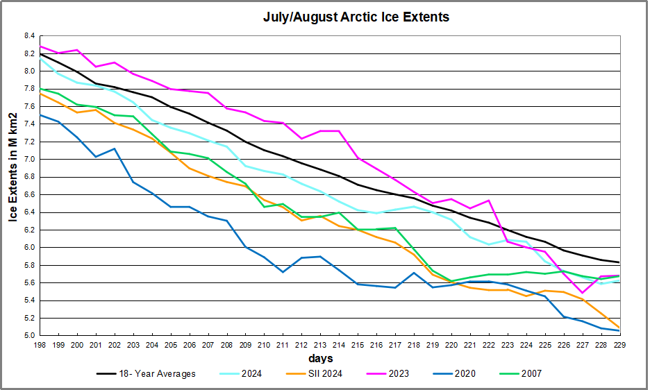
The table below shows the distribution of Sea Ice on day 229 across the Arctic Regions, on average, this year and 2007. At this point in the year, Bering and Okhotsk seas are open water and thus dropped from the table.

Region 2024229 Day 229 Ave 2024-Ave. 2007229 2024-2007
 (0) Northern_Hemisphere 5623262 5828731 -205469 5673531 -50270
 (1) Beaufort_Sea 591190 698788 -107598 767181 -175991
 (2) Chukchi_Sea 554701 425156 129544 253092 301609
 (3) East_Siberian_Sea 641562 535416 106146 154536 487026
 (4) Laptev_Sea 268971 240911 28059 284910 -15939
 (5) Kara_Sea 14414 96702 -82288 201203 -186789
 (6) Barents_Sea 0 21833 -21833 17229 -17229
 (7) Greenland_Sea 120478 216573 -96095 310070 -189591
 (8) Baffin_Bay_Gulf_of_St._Lawrence 46366 53298 -6932 75105 -28739
 (9) Canadian_Archipelago 319281 399712 -80431 382407 -63126
 (10) Hudson_Bay 33319 58874 -25555 89354 -56034
 (11) Central_Arctic 3031923 3080445 -48523 3137188.82 -105266

The overall deficit to average is 205k km2, (3.5%).  The major deficits are in  Beaufort, Kara, Greenland Sea and CAA (Canadian Archipelago), partly offset by surpluses in Chukchi and East Siberian.

For more on the differences between MASIE and SII see this post:

Support MASIE Arctic Ice Dataset

bathymetric_map_arctic_ocean

Illustration by Eleanor Lutz shows Earth’s seasonal climate changes. If played in full screen, the four corners present views from top, bottom and sides. It is a visual representation of scientific datasets measuring ice and snow extents.

There is no charge for content on this site, nor for subscribers to receive email notifications of postings.