Prevous posts provided the context regarding the Climate Tutorial requested by Judge Alsup in the lawsuit case filed by California cities against big oil companies: Cal Court to Hear Climate Tutorial
An overview of a submission by Professors Happer, Koonin and Lindzen was in Climate Tutorial for Judge Alsup
This post goes into the meat and potatoes of that submission with excerpts from Section II: Answers to specific questions (my bolds)
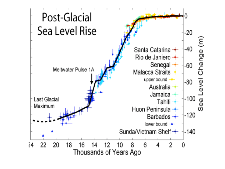
Question 1: What caused the various ice ages (including the “little ice age” and prolonged cool periods) and what caused the ice to melt? When they melted, by how much did sea level rise?
The discussion of the major ice ages of the past 700 thousand years is distinct from the discussion of the “little ice age.” The former refers to the growth of massive ice sheets (a mile or two thick) where periods of immense ice growth occurred, lasting approximately eighty thousand years, followed by warm interglacials lasting on the order of twenty thousand years. By contrast, the “little ice age” was a relatively brief period (about four hundred years) of relatively cool temperatures accompanied by the growth of alpine glaciers over much of the earth.

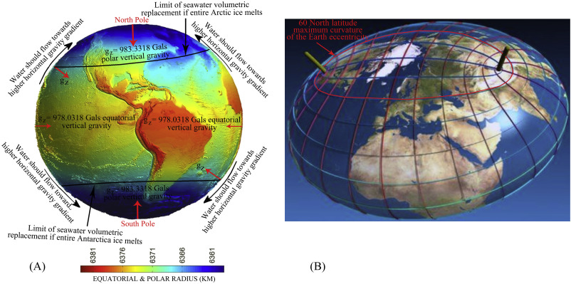
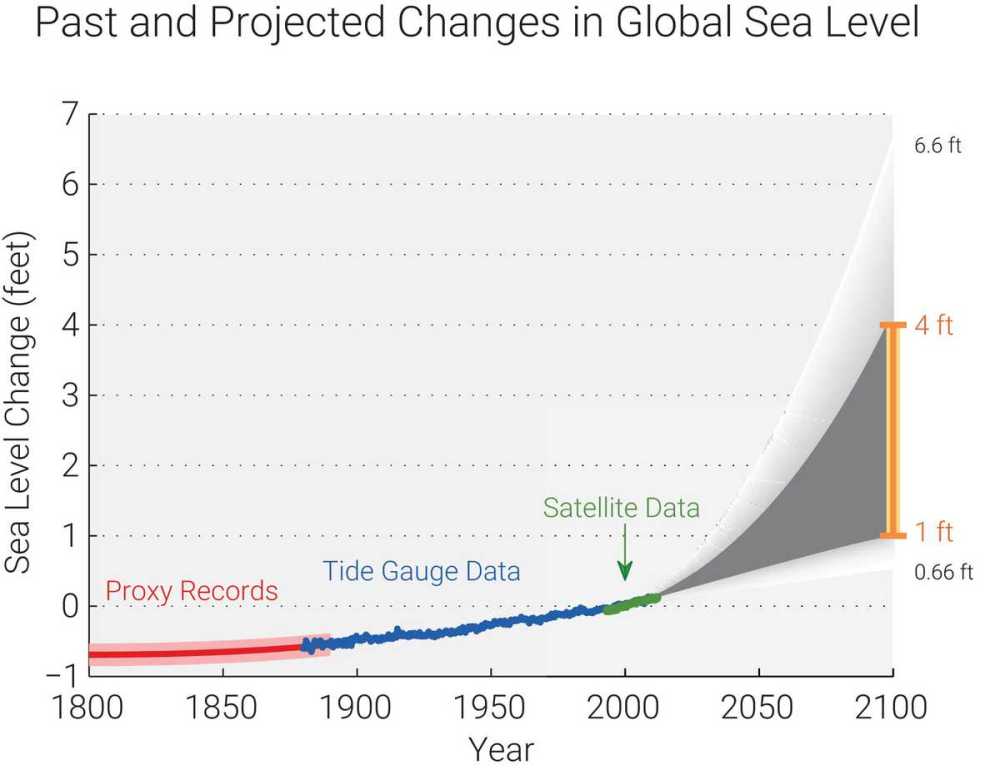
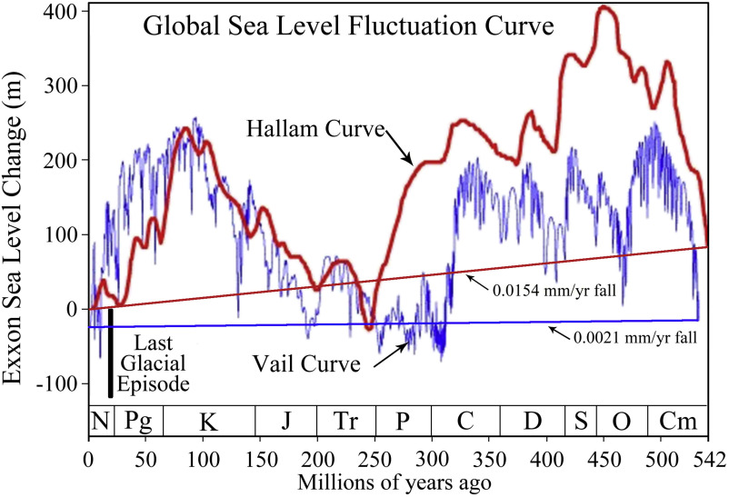
The last glacial episode ended somewhat irregularly. Ice coverage reached its maximum extent about eighteen thousand years ago. Melting occurred between about twenty thousand years ago and thirteen thousand years ago, and then there was a strong cooling (Younger Dryas) which ended about 11,700 years ago. Between twenty thousand years ago and six thousand years ago, there was a dramatic increase in sea level of about 120 meters followed by more gradual increase over the following several thousand years. Since the end of the “little ice age,” there has been steady increase in sea-level of about 6 inches per century.
As to the cause of the “little ice age,” this is still a matter of uncertainty. There was a long hiatus in solar activity that may have played a role, but on these relatively short time scales one can’t exclude natural internal variability. It must be emphasized that the surface of the earth is never in equilibrium with net incident solar radiation because the oceans are always carrying heat to and from the surface, and the motion systems responsible have time scales ranging from years (for example ENSO) to millennia.
The claim that orbital variability requires a boost from CO2 to drive ice ages comes from the implausible notion that what matters is the orbital variations in the global average insolation (which are, in fact, quite small) rather than the large forcing represented by the Milankovitch parameter. This situation is very different than in the recent and more modest shorter-term warming, where natural variability makes the role of CO2 much more difficult to determine.
Question 2: What is the molecular difference by which CO2 absorbs infrared radiation but oxygen and nitrogen do not?
Molecules like CO2, H2O, CO or NO are called a greenhouse-gas molecules, because they can efficiently absorb or emit infrared radiation, but they are nearly transparent to sunlight. Molecules like O2 and N2 are also nearly transparent to sunlight, but since they do not absorb or emit thermal infrared radiation very well, they are not greenhouse gases. The most important greenhouse gas, by far, is water vapor. Water molecules, H2O, are permanently bent and have large electric dipole moments.
Question 3: What is mechanism by which infrared radiation trapped by CO2 in the atmosphere is turned into heat and finds its way back to sea level?
Unscattered infrared radiation is very good at transmitting energy because it moves at the speed of light. But the energy per unit volume stored by the thermal radiation in the Earth’s atmosphere is completely negligible compared to the internal energy of the air molecules.
Although CO2 molecules radiate very slowly, there are so many CO2 molecules that they produce lots of radiation, and some of this radiation reaches sea level. The figure following shows downwelling radiation measured at the island of Nauru in the Tropical Western Pacific Ocean, and at colder Point Barrow, Alaska, on the shore of the Arctic Ocean.
So the answer to the last part of the question, “What is the mechanism by which … heat … finds its way back to sea level?” is that the heat is radiated to the ground by molecules at various altitudes, where there is usually a range of different temperatures. The emission altitude is the height from which radiation could reach the surface without much absorption, say 50% absorption. For strongly absorbed frequencies, the radiation reaching the ground comes from low-altitude molecules, only a few meters above ground level for the 667 cm-1 frequency at the center of the CO2 band. More weakly absorbed frequencies are radiated from higher altitudes where the temperature is usually colder than that of the surface. But occasionally, as the data from Point Barrow show, higher-altitude air can be warmer than the surface.

Closely related to Question 3 is how heat from the absorption of sunlight by the surface gets back to space to avoid a steadily increasing surface temperature. As one might surmise from the figure, at Narau there is so much absorption from CO2 and by water vapor, H2O, that most daytime heat transfer near the surface is by convection, not by radiation. Especially important is moist convection, where the water vapor in rising moist air releases its latent heat to form clouds. The clouds have a major effect on radiative heat transfer. Cooled, drier, subsiding air completes the convection circuit. Minor changes of convection and cloudiness can have a bigger effect on the surface temperature than large changes in CO2 concentrations.
Question 4: Does CO2 in the atmosphere reflect any sunlight back into space, such that the reflected sunlight never penetrates the atmosphere in the first place?
The short answer to this question is “No”, but it raises some interesting issues that we discuss below.
Molecules can either scatter or absorb radiation. CO2 molecules are good absorbers of thermal infrared radiation, but they scatter almost none. Infrared radiant energy absorbed by a CO2 molecule is converted to internal vibrational and rotational energy. This internal energy is quickly lost in collisions with the N2 and O2 molecules that make up most of the atmosphere. The collision rates, billions per second, are much too fast to allow the CO2 molecules to reradiate the absorbed energy, which takes about a second. CO2 molecules in the atmosphere do emit thermal infrared radiation continuously, but the energy is almost always provided by collisions with N2 and O2 molecules, not by previously absorbed radiation. The molecules “glow in the dark” with thermal infrared radiation.
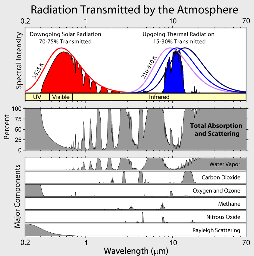
The figure shows that water vapor is by far the most important absorber. It can absorb both thermal infrared radiation from the Earth and shorter-wave radiation from the Sun. Water vapor and its condensates, clouds of liquid or solid water (ice), dominate radiative heat transfer in the Earth’s atmosphere; CO2 is of secondary importance.
If Question 4 were “Do clouds in the atmosphere reflect any sunlight back into space, such that the reflected sunlight never penetrates the atmosphere in the first place?” the answer would be “Yes”. It is common knowledge that low clouds on a sunny day shade and cool the surface of the Earth by scattering the sunlight back to space before it can be absorbed and converted to heat at the surface.
The figure shows that very little thermal radiation from the surface can reach the top of the atmosphere without absorption, even if there are no clouds. But some of the surface radiation is replaced by molecular radiation emitted by greenhouse molecules or cloud tops at sufficiently high altitudes that the there are no longer enough higher-altitude greenhouse molecules or clouds to appreciably attenuate the radiation before it escapes to space. Since the replacement radiation comes from colder, higher altitudes, it is less intense and does not reject as much heat to space as the warmer surface could have without greenhousegas absorption.
As implied by the figure, sunlight contains some thermal infrared energy that can be absorbed by CO2. But only about 5% of sunlight has wavelengths longer than 3 micrometers where the strongest absorption bands of CO2 are located. The Sun is so hot, that most of its radiation is at visible and near-visible wavelengths, where CO2 has no absorption bands.
Question 5: Apart from CO2, what happens to the collective heat from tail pipe exhausts, engine radiators, and all other heat from combustion of fossil fuels? How, if at all, does this collective heat contribute to warming of the atmosphere?
After that energy is used for heat, mobility, and electricity, the Second Law of Thermodynamics guarantees that virtually all of it ends up as heat in the climate system, ultimately to be radiated into space along with the earth’s natural IR emissions. [A very small fraction winds up as visible light that escapes directly to space through the transparent atmosphere, but even that ultimately winds up as heat somewhere “out there.”]

How much does this anthropogenic heat affect the climate? There are local effects where energy use is concentrated, for example in cities and near power plants. But globally, the effects are very small. To see that, convert the global annual energy consumption of 13.3 Gtoe (Gigatons of oil equivalent) to 5.6 × 10^20 joules. Dividing that by the 3.2 × 10^7 seconds in a year gives a global power consumption of 1.75 × 10^13 Watts. Spreading that over the earth’s surface area of 5.1 × 10^14 m2 results in an anthropogenic heat flux of 0.03 W/m2 . This is some four orders of magnitude smaller than the natural heat fluxes of the climate system, and some two orders of magnitude smaller than the anthropogenic radiative forcing.
Question 6: In grade school many of us were taught that humans exhale CO2 but plants absorb CO2 and return oxygen to the air (keeping the carbon fiber). Is this still valid? If so why hasn’t plant life turned the higher levels of CO2 back into oxygen? Given the increase in population on earth (four billion), is human respiration a contributing factor to the buildup of CO2?
If all of the CO2 produced by current combustion of fossil fuels remained in the atmosphere, the level would increase by about 4 ppm per year, substantially more than the observed rate of around 2.5 ppm per year, as seen in the figure above. Some of the anthropogenic CO2 emissions are being sequestered on land or in the oceans.

There is evidence that primary photosynthetic productivity has increased somewhat over the past half century, perhaps due to more CO2 in the atmosphere. For example, the summerwinter swings like those in the figure above are increasing in amplitude. Other evidence for modestly increasing primary productivity includes the pronounced “greening” of the Earth that has been observe by satellites. An example is the map above, which shows a general increase in vegetation cover over the past three decades.
The primary productivity estimate mentioned above would also correspond to an increase of the oxygen fraction of the air by 50 ppm, but since the oxygen fraction of the air is very high (209,500 ppm), the relative increase would be small and hard to detect. Also much of the oxygen is used up by respiration.
The average human exhales about 1 kg of CO2 per day, so the 7 billion humans that populate the Earth today exhale about 2.5 x 10^9 tons of CO2 per year, a little less than 1% of that is needed to support the primary productivity of photosynthesis and only about 6% of the CO2 “pollution” resulting from the burning of fossil fuels. However, unlike fossil fuel emissions, these human (or more generally, biological) emissions do not accumulate in the atmosphere, since the carbon in food ultimately comes from the atmosphere in the first place.
Question 7: What are the main sources of CO2 that account for the incremental buildup of CO2 in the atmosphere?
The CO2 in the atmosphere is but one reservoir within the global carbon cycle, whose stocks and flows are illustrated by Figure 6.1 from IPCC AR5 WG1:

There is a nearly-balanced annual exchange of some 200 PgC between the atmosphere and the earth’s surface (~80 Pg land and ~120 Pg ocean); the atmospheric stock of 829 Pg therefore “turns over” in about four years.
Human activities currently add 8.9 PgC each year to these closely coupled reservoirs (7.8 from fossil fuels and cement production, 1.1 from land use changes such as deforestation). About half of that is absorbed into the surface, while the balance (airborne fraction) accumulates in the atmosphere because of its multicentury lifetime there. Other reservoirs such as the intermediate and deep ocean are less closely coupled to the surface-atmosphere system.
Much of the natural emission of CO2 stems from the decay of organic matter on land, a process that depends strongly on temperature and moisture. And much CO2 is absorbed and released from the oceans, which are estimated to contain about 50 times as much CO2 as the atmosphere. In the oceans CO2 is stored mostly as bicarbonate (HCO3 – ) and carbonate (CO3 – – ) ions. Without the dissolved CO2, the mildly alkaline ocean with a pH of about 8 would be very alkaline with a pH of about 11.3 (like deadly household ammonia) because of the strong natural alkalinity.
Only once in the geological past, the Permian period about 300 million years ago, have atmospheric CO2 levels been as low as now. Life flourished abundantly during the geological past when CO2 levels were five or ten times higher than those today.
Question 8: What are the main sources of heat that account for the incremental rise in temperature on earth?
The only important primary heat source for the Earth’s surface is the Sun. But the heat can be stored in the oceans for long periods of time, even centuries. Variable ocean currents can release more or less of this stored heat episodically, leading to episodic rises (and falls) of the Earth’s surface temperature.
Incremental changes of the surface temperature anomaly can be traced back to two causes: (1) changes in the surface heating rate; (2) changes in the resistance of heat flow to space. Quasi periodic El Nino episodes are examples of the former. During an El Nino year, easterly trade winds weaken and very warm deep water, normally blown toward the coasts of Indonesia and Australia, floats to the surface and spreads eastward to replace previously cool surface waters off of South America. The average temperature anomaly can increase by 1 C or more because of the increased release of heat from the ocean. The heat source for the El Nino is solar energy that has accumulated beneath the ocean surface for several years before being released.

On average, the absorption rate of solar radiation by the Earth’s surface and atmosphere is equal to emission rate of thermal infrared radiation to space. Much of the radiation to space does not come from the surface but from greenhouse gases and clouds in the lower atmosphere, where the temperature is usually colder than the surface temperature, as shown in the figure on the previous page. The thermal radiation originates from an “escape altitude” where there is so little absorption from the overlying atmosphere that most (say half) of the radiation can escape to space with no further absorption or scattering. Adding greenhouse gases can warm the Earth’s surface by increasing the escape altitude. To maintain the same cooling rate to space, the temperature of the entire troposphere, and the surface, would have to increase to make the effective temperature at the new escape altitude the same as at the original escape altitude. For greenhouse warming to occur, a temperature profile that cools with increasing altitude is required.
Over most of the CO2 absorption band (between about 580 cm-1 and 750 cm-1 ) the escape altitude is the nearly isothermal lower stratosphere shown in the first figure. The narrow spike of radiation at about 667 cm-1 in the center of the CO2 band escapes from an altitude of around 40 km (upper stratosphere), where it is considerably warmer than the lower stratosphere due heating by solar ultraviolet light which is absorbed by ozone, O3. Only at the edges of the CO2 band (near 580 cm-1 and 750 cm-1 ) is the escape altitude in the troposphere where it could have some effect on the surface temperature. Water vapor, H2O, has emission altitudes in the troposphere over most of its absorption bands. This is mainly because water vapor, unlike CO2, is not well mixed but mostly confined to the troposphere.
Summary
To summarize this overview, the historical and geological record suggests recent changes in the climate over the past century are within the bounds of natural variability. Human influences on the climate (largely the accumulation of CO2 from fossil fuel combustion) are a physically small (1%) effect on a complex, chaotic, multicomponent and multiscale system. Unfortunately, the data and our understanding are insufficient to usefully quantify the climate’s response to human influences. However, even as human influences have quadrupled since 1950, severe weather phenomena and sea level rise show no significant trends attributable to them. Projections of future climate and weather events rely on models demonstrably unfit for the purpose. As a result, rising levels of CO2 do not obviously pose an immediate, let alone imminent, threat to the earth’s climate.
Full text of submission is here

 The data is annual averages of absolute SSTs measured in the North Atlantic. The significance of the pulses for weather forecasting is discussed in
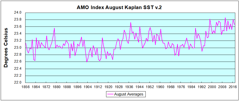


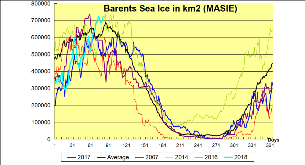
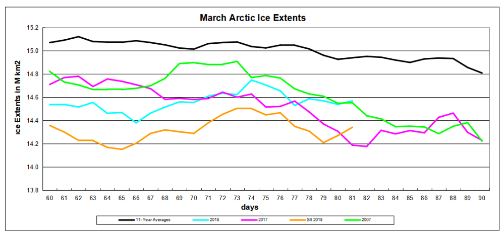
 After a slow beginning this month, Arctic ice advanced to set a late annual maximum, and is now holding on to its gains the last four days. The image above shows the last week, setting new 2018 maximums on day 74 for NH overall, as well in Barents Sea. The graph below shows that as of yesterday, Barents is well above the 11 year average, and matching 2014 the highest year in the decade.