Click on image to enlarge.
With 2017 ice extent estimates complete we can look at the year in perspective. Above is a graph showing the annual average extents since 2007, comparing MASIE and SII (v3.0). Obviously, the trend in MASIE could not be flatter, while SII shows a decline. The first five years the two indices were nearly the same, and since then SII shows less ice, about 260k km2 each year. Note also how small is the variance year over year: Standard deviation is +/- 260k km2, or about 2.5% of the average annual extent. This holds for both indices. Note also a pattern of three higher years followed by two lower years.
A previous post Sea Ice Index Updates to v.3.0 reported on the newest SII version, and we can see how it compares with MASIE over this last year.

Click on image to enlarge.
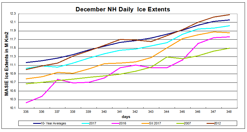
The first four months show more diversity, both in the 10 year averages and in 2017 results. From May on MASIE 2017 tracks closely to its average, while SII shows 2017 below its average every month. For those who want to see the numbers a table is provided below.
| Units |
2007
to 2016 |
2017 |
2007
to 2016 |
2017 |
| M km2 |
MASIE |
MASIE |
SII |
SII |
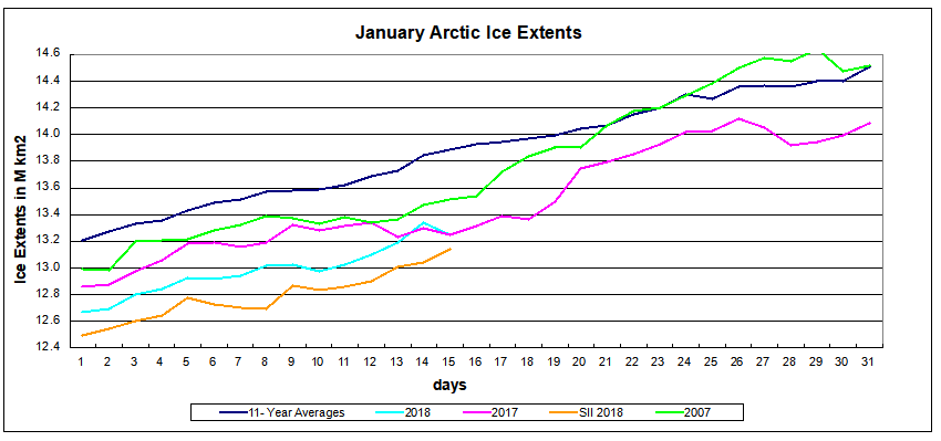
| Jan |
13.921 |
13.503 |
13.686 |
13.174 |
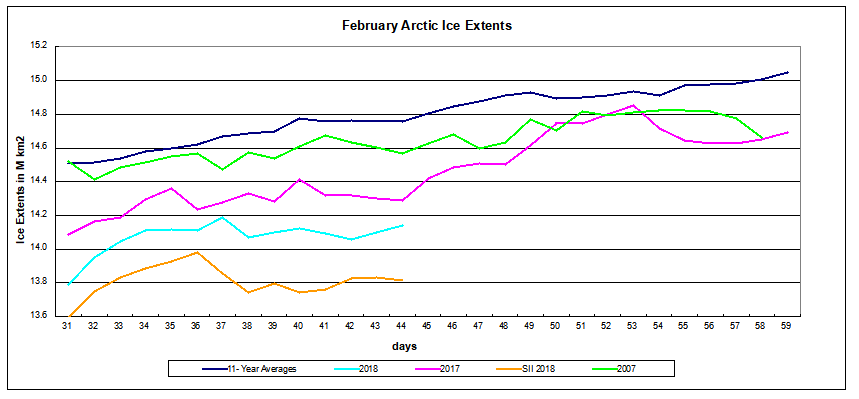
| Feb |
14.841 |
14.478 |
14.553 |
14.112 |
| Mar |
15.053 |
14.509 |
14.815 |
14.273 |
| Apr |
14.353 |
13.941 |
14.206 |
13.760 |
| May |
12.763 |
12.838 |
12.757 |
12.618 |
| June |
10.906 |
10.975 |
10.938 |
10.720 |
| July |
8.359 |
8.383 |
8.107 |
7.901 |
| Aug |
5.955 |
6.006 |
5.657 |
5.472 |
| Sept |
4.663 |
4.832 |
4.676 |
4.797 |
| Oct |
6.630 |
6.804 |
6.734 |
6.715 |
| Nov |
9.897 |
9.697 |
9.718 |
9.458 |
| Dec |
12.235 |
11.972 |
12.063 |
11.752 |
| Annual Ave. |
10.798 |
10.661 |
10.659 |
10.396 |
Some are proclaiming dire warnings about melting ice and imagining various dangerous impacts. Some fluctuations do appear but not very large and somewhat cyclical. Since 2007 it resembles a plateau more than anything else.
Background on MASIE Data Sources
MASIE reports are generated by National Ice Center from the Interactive Multisensor Snow and Ice Mapping System (IMS). From the documentation, the multiple sources feeding IMS are:
Platform(s) AQUA, DMSP, DMSP 5D-3/F17, GOES-10, GOES-11, GOES-13, GOES-9, METEOSAT, MSG, MTSAT-1R, MTSAT-2, NOAA-14, NOAA-15, NOAA-16, NOAA-17, NOAA-18, NOAA-N, RADARSAT-2, SUOMI-NPP, TERRA
Sensor(s): AMSU-A, ATMS, AVHRR, GOES I-M IMAGER, MODIS, MTSAT 1R Imager, MTSAT 2 Imager, MVIRI, SAR, SEVIRI, SSM/I, SSMIS, VIIRS
Summary: IMS Daily Northern Hemisphere Snow and Ice Analysis
The National Oceanic and Atmospheric Administration / National Environmental Satellite, Data, and Information Service (NOAA/NESDIS) has an extensive history of monitoring snow and ice coverage.Accurate monitoring of global snow/ice cover is a key component in the study of climate and global change as well as daily weather forecasting.
The Polar and Geostationary Operational Environmental Satellite programs (POES/GOES) operated by NESDIS provide invaluable visible and infrared spectral data in support of these efforts. Clear-sky imagery from both the POES and the GOES sensors show snow/ice boundaries very well; however, the visible and infrared techniques may suffer from persistent cloud cover near the snowline, making observations difficult (Ramsay, 1995). The microwave products (DMSP and AMSR-E) are unobstructed by clouds and thus can be used as another observational platform in most regions. Synthetic Aperture Radar (SAR) imagery also provides all-weather, near daily capacities to discriminate sea and lake ice. With several other derived snow/ice products of varying accuracy, such as those from NCEP and the NWS NOHRSC, it is highly desirable for analysts to be able to interactively compare and contrast the products so that a more accurate composite map can be produced.
The Satellite Analysis Branch (SAB) of NESDIS first began generating Northern Hemisphere Weekly Snow and Ice Cover analysis charts derived from the visible satellite imagery in November, 1966. The spatial and temporal resolutions of the analysis (190 km and 7 days, respectively) remained unchanged for the product’s 33-year lifespan.
As a result of increasing customer needs and expectations, it was decided that an efficient, interactive workstation application should be constructed which would enable SAB to produce snow/ice analyses at a higher resolution and on a daily basis (~25 km / 1024 x 1024 grid and once per day) using a consolidated array of new as well as existing satellite and surface imagery products. The Daily Northern Hemisphere Snow and Ice Cover chart has been produced since February, 1997 by SAB meteorologists on the IMS.
Another large resolution improvement began in early 2004, when improved technology allowed the SAB to begin creation of a daily ~4 km (6144×6144) grid. At this time, both the ~4 km and ~24 km products are available from NSIDC with a slight delay. Near real-time gridded data is available in ASCII format by request.
In March 2008, the product was migrated from SAB to the National Ice Center (NIC) of NESDIS. The production system and methodology was preserved during the migration. Improved access to DMSP, SAR, and modeled data sources is expected as a short-term from the migration, with longer term plans of twice daily production, GRIB2 output format, a Southern Hemisphere analysis, and an expanded suite of integrated snow and ice variable on horizon.
http://www.natice.noaa.gov/ims/ims_1.html
Footnote
Some people unhappy with the higher amounts of ice extent shown by MASIE continue to claim that Sea Ice Index is the only dataset that can be used. This is false in fact and in logic. Why should anyone accept that the highest quality picture of ice day to day has no shelf life, that one year’s charts can not be compared with another year? Researchers do this, including Walt Meier in charge of Sea Ice Index. That said, I understand his interest in directing people to use his product rather than one he does not control. As I have said before:
MASIE is rigorous, reliable, serves as calibration for satellite products, and continues the long and honorable tradition of naval ice charting using modern technologies. More on this at my post Support MASIE Arctic Ice Dataset


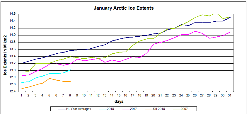
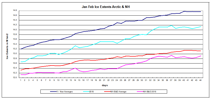 Clearly the deficit to average is mostly due to B&O, and as the table below shows, mostly Bering at this point.


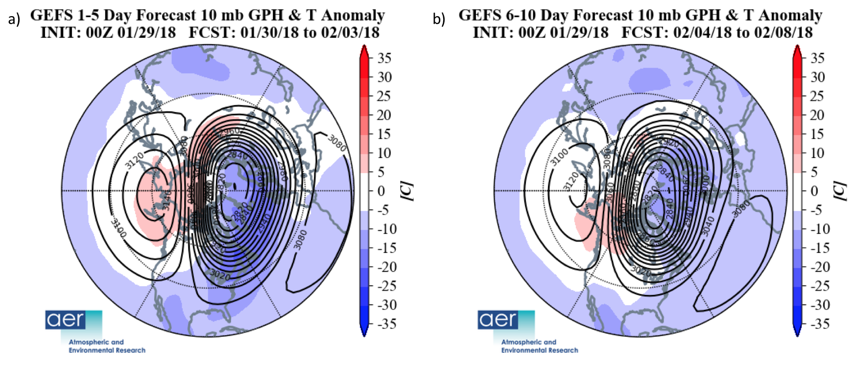
 I am excerpting from Dr. Cohen’s latest post because of his refreshing candor sharing his thought processes regarding arctic weather patterns.