Everywhere Elsewhere Climate Claims

We often hear reports that something is occurring around the world, and then someone responds: “That’s not happening where I live.” And the rebuttal is, “Your neighborhood is not typical of the rest of the world.” In other words, the claim is: this trend is going on everywhere elsewhere despite your not observing it.

For a month now we have been reading in the media about how July was the hottest month in recorded history.

“July was Earth’s hottest month on record, NOAA says” http://www.bbc.com/news/world-us-canada-34009289

And at the same time, we read reports about how cool the summer was in Canada, in the US, in the UK, in parts of Europe and how cold was the winter in Australia.

“What a washout! A British summer to forget. In the UK July was colder than average, and we had 140% of average rainfall.” http://www.theguardian.com/uk-news/2015/aug/16/washout-british-summer-witness-holiday-experts

“The July contiguous U.S. average temperature was 73.9°F, 0.2°F above the 20th century average and ranked near the middle in the 121-year period of record.” http://www.ncdc.noaa.gov/sotc/national/201507

“Wetter than normal summer for most of Canada except B.C.” http://www.vancitybuzz.com/2015/08/wetter-than-normal-summer-canada-except-bc/

“A large swath stretching from eastern Scandinavia into western Siberia was cooler than average, with part of western Russia much cooler than average. Cooler than average temperatures were also observed across parts of eastern and southern Asia and scattered areas in central and northern North America.” (Source: NOAA)

So the question arises: Is there global warming unseen in most observations? How would we know what was observed in July and whether it was unusual or not?

NOAA provides this analysis of July 2015.

Continental Temperature Anomalies July 2015

CONTINENT ANOMALY (1910-2000) TREND (1910-2015) RANK
°C °F °C °F (OUT OF 106 YEARS)
North America 0.53 0.95 0.08 0.14 Warmest 16ᵗʰ
Coolest 90ᵗʰ
Ties: 1941
South America 1.43 2.57 0.14 0.25 Warmest 5ᵗʰ
Coolest 102ⁿᵈ
Europe 1.53 2.75 0.12 0.21 Warmest 6ᵗʰ
Coolest 101ˢᵗ
Africa 1.2 2.16 0.1 0.18 Warmest 2ⁿᵈ
Coolest 105ᵗʰ
Asia 0.7 1.26 0.07 0.13 Warmest 10ᵗʰ
Coolest 97ᵗʰ
Oceania 0.57 1.03 0.11 0.19 Warmest 26ᵗʰ
Coolest 81ˢᵗ

https://www.ncdc.noaa.gov/sotc/global-regions/201507

The table shows that no continent had the warmest July ever.  Africa came close and also South America, which means a milder mid-winter than usual in the southern hemisphere.  So how come they claim a record July?

The answer is provided by another NOAA analysis.

Global Analysis of July 2015

JULY ANOMALY RANK RECORDS
°C °F (OUT OF 136 YEARS) YEAR(S) °C °F
Global
Land +0.96 ± 0.18 +1.73 ± 0.32 Warmest 6th 1998 1.11 2
Coolest 131st 1884 -0.68 -1.22
Ocean +0.75 ± 0.07 +1.35 ± 0.13 Warmest 1st 2015 0.75 1.35
Coolest 136th 1911 -0.5 -0.9
Land and Ocean +0.81 ± 0.14 +1.46 ± 0.25 Warmest 1st 2015 0.81 1.46
Coolest 136th 1904, 1911 -0.47 -0.85


So there you have it.  Once again the ocean is making the climate, with July SSTs higher because of the Blob and the long-developing El Nino.  And we can expect that with all the heat now being released upward from the water, there will be cooling of SSTs and a La Nina in response.

Climate Models Explained

A comment by Dr. R.G. Brown of Duke University posted on June 11 at WUWT.

noaa climate model

Overview of the structure of a state-of-the-art climate model. From the NOAA website http://www.research.noaa.gov/climate/t_modeling.html

First about the way weather models work

That is not quite what they do in GCMs. There are two reasons for this. One is that a global grid of 2 million temperatures sounds like a lot, but it’s not. Remember the atmosphere has depth, and they have to initialize at least to the top of the troposphere, and if they use 1 km thick cells there are 9 or 10 layers. Say 10. Then they have 500 million square kilometers of area to cover. Even if the grid itself has two million cells, that is still cells that contain 250 square km. This isn’t terrible — 16x16x1 km cells (20 million of them assuming they follow the usual practice of slabs 1 km thick) are small enough that they can actually resolve largish individual thunderstorms — but is still orders of magnitude larger than distinct weather features like individual clouds or smaller storms or tornadoes or land features (lakes, individual hills and mountains) that can affect the weather.

There is also substantial error in their initial conditions — as you say, they smooth temperatures sampled at a lot fewer than 2 million points to cover vast tracts of the grid where there simply are no thermometers, and even where they have surface thermometers they do not generally have soundings (temperature measurements from e.g. balloons that ride up the air column at a location) so they do not know the temperature in depth. The model initialization has to do things like take the surface temperature guess (from a smoothing model) and guess the temperature profile overhead using things like the adiabatic lapse rate, a comparative handful of soundings, knowledge of the cloudiness or whatever of the cell obtained from satellite or radar (where available) or just plain rules of thumb (all built into a model to initialize the model.

Then there is the ocean. Sea surface temperatures matter a great deal, but so do temperatures down to some depth (more for climate than for weather, but when large scale phenomena like hurricanes come along, the heat content of the ocean down to some depth very much plays a role in their development) so they have to model that, and the better models often contain at least one if not more layers down into the dynamic ocean. The Gulf Stream, for example, is a river in the Atlantic that transports heat and salinity and moves around 200 kilometers in a day on the surface, less at depth, which means that fluctuations in surface temperature, fed back or altered by precipitation or cloudiness or wind, move across many cells over the course of a day.  (My Bold)

Even with all of the care I describe above and then some, weather models computed at close to the limits of our ability to compute (and get a decent answer faster than nature “computes” it by making it actually happen) track the weather accurately for a comparatively short time — days — before small variations between the heavily modeled, heavily under-sampled model initial conditions and the actual initial state of the weather plus errors in the computation due to many things — discrete arithmetic, the finite grid size, errors in the implementation of the climate dynamics at the grid resolution used (which have to be approximated in various ways to “mimic” the neglected internal smaller scaled dynamics that they cannot afford to compute) cause the models to systematically diverge from the actual weather.

If they run the model many times with small tweaks of the initial conditions, they have learned empirically that the distribution of final states they obtain can be reasonably compared to the climate for a few days more in an increasingly improbable way, until around a week or ten days out the variation is so great that they are just as well off predicting the weather by using the average weather for a date over the last 100 years and a bit of sense, just as is done in almanacs.

In other words, the models, no matter how many times they are run or how carefully they are initialized, produce results with no “lift” over ordinary statistics at around 10 days. (My bold)

Evolution of state-of-the-art Climate Models from the mid 70s to the mid 00s. From IPCC (2007)

Evolution of state-of-the-art Climate Models from the mid 70s to the mid 00s. From IPCC (2007)

Now How Climate Models Work:

Then here is the interesting point. Climate models are just weather models run in exactly this way, with one exception. Since they know that the model will produce results indistinguishable from ordinary static statistics two weeks in, they don’t bother initializing them all that carefully. The idea is that no matter how then initialize them, after running them out to weeks or months the bundle of trajectories they produce from small perturbations will statistically “converge” at any given time to what is supposed to be the long time statistical average, which is what they are trying to predict.

This assumption is itself dubious, as neither the weather nor the climate is stationary and it is most definitely non-Markovian so that the neglected details in the initial state do matter in the evolution of both, and there is also no theorem of which I am aware that states that the average or statistical distribution of a bundle of trajectories generated from a nonlinear chaotic model of this sort will in even the medium run be an accurate representation of the nonstationary statistical distribution of possible future climates. But it’s the only game in town, so they give it a try.

They then run this re-purposed, badly initialized weather model out until they think it has had time to become a “sample” for the weather for some stationary initial condition (fixed date, sunlight, atmosphere, etc) and then they vary things like CO_2 systematically over time while integrating and see how the run evolves over future decades. The bundle of future climate trajectories thus generated from many tweaks of initial conditions and sometimes the physical parameters as well is then statistically analyzed, and its mean becomes the central prediction of the model and the variance or envelope of all of the trajectories become confidence intervals of its predictions.

The problem is that they aren’t really confidence intervals because we don’t really have any good reason to think that the integration of the weather ten years into the future at an inadequate grid size, with all of the accumulation of error along the way, is actually a sample from the same statistical distribution that the real weather is being drawn from subject to tiny perturbations in its initial state. The climate integrates itself down to the molecular level, not on a 16×16 km grid, and climate models can’t use that small a grid size and run in less than infinite time, so the highest resolution I’ve heard of is 100×100 km^2 cells (10^4 square km, which is around 50,000 cells, not two million).

At this grid size they cannot see individual thunderstorms at all. Indeed, many extremely dynamic features of heat transport in weather have to be modeled by some sort of empirical “mean field” approximation of the internal cell dynamics — “average thunderstormicity” or the like as thunderstorms in particular cause rapid vertical transport of a lot of heat up from the surface and rapid transport of chilled/chilling water down to the surface, among other things. The same is true of snowpack — even small errors in average snowpack coverage make big differences in total heat received in any given winter and this can feed back to kick a model well off of the real climate in a matter of years.

So far, it looks like (not unlike the circumstance with weather) climate models can sometimes track the climate for a decade or so before they diverge from it.   (My Bold)

They suffer from many other ailments as well — if one examines the actual month to month or year to year variance of the “weather” they predict, it has the wrong amplitude and decay times compared to the actual climate, which is basically saying (via the fluctuation-dissipation theorem) that they have the physics of the open system wrong. The models heavily exaggerate the effect of aerosols and tend to overreact to things like volcanic eruptions that dump aerosols into the atmosphere.

The models are tuned to cancel the exaggerated effect of aerosols with an exaggerated feedback on top of CO_2 driven warming to make them “work” to track the climate over a 20 year reference period. Sadly, this 20 year reference period was chosen to be the single strongest warming stretch of the 20th century, ignoring cooling periods and warming periods that preceded it and (probably as a consequence) diverging from the flat-to-slightly cooling period we’ve been in for the last 16 or so years (or more, or less, depending on who you are talking to, but even the IPCC formally recognizes “the pause, the hiatus”, the lack of warming for this interval, in AR5. It is a serious problem for the models and everybody knows it.

The IPCC then takes the results of many GCMs and compounds all errors by super-averaging their results (which has the effect of hiding the fluctuation problem from inquiring eyes), ignoring the fact that some models in particular truly suck in all respects at predicting the climate and that others do much better, because the ones that do better predict less long run warming and that isn’t the message they want to convey to policy makers, and transform its envelope into a completely unjustifiable assertion of “statistical confidence”.

This is a simple lie. Each model one at a time can have the confidence interval produced by the spread in long-run trajectories produced by the perturbation of its initial conditions compared to the actual trajectory of the climate and turned into a p-value. The p-value is a measure of the probability of the truth of the null hypothesis — “This climate model is a perfect model in that its bundle of trajectories is a representation of the actual distribution of future climates”. This permits the estimation of the probability of getting our particular real climate given this distribution, and if the probability is low, especially if it is very low, we under ordinary circumstances would reject the huge bundle of assumptions tied up in as “the hypothesis” represented by the model itself and call the model “failed”, back to the drawing board.

One cannot do anything with the super-average of 36 odd non-independent grand average per-model results. To even try to apply statistics to this shotgun blast of assumptions one has to use something called the Bonferroni correction, which basically makes the p-value for failure of individual models in the shotgun blast much, much larger (because they have 36 chances to get it right, which means that even if all 36 are wrong pure chance can — no, probably will — make a bad model come out within a p = 0.05 cutoff as long as the models aren’t too wrong yet.

By this standard, “the set of models in CMIP5″ has long since failed. There isn’t the slightest doubt that their collective prediction is statistical nonsense. It remains to be seen if individual models in the collection deserve to be kept in the running as not failed yet, because even applying the Bonferroni correction to the “ensemble” of CMIP5 is not good statistical practice. Each model should really be evaluated on its own merits as one doesn’t expect the “mean” or “distribution” of individual model results to have any meaning in statistics (note that this is NOT like perturbing the initial conditions of ONE model, which is a form of Monte Carlo statistical sampling and is something that has some actual meaning).

Hope this helps.

rgb
http://wattsupwiththat.com/2015/06/09/huge-divergence-between-latest-uah-and-hadcrut4-revisions-now-includes-april-data/#comment-1960561

In the conclusion of a recent paper, Valerio Lucarini adds:

We have briefly recapitulated some of the scientific challenges and epistemological issues related to climate science. We have discussed the formulation and testing of theories and numerical models, which, given the presence of unavoidable uncertainties in observational data, the nonrepeatability of world-experiments, and the fact that relevant processes occur in a large variety of spatial and temporal scales, require a rather different approach than in other scientific contexts.

In particular, we have clarified the presence of two different levels of unavoidable uncertainties when dealing with climate models, related to the complexity and chaoticity of the system under investigation. The first is related to the imperfect knowledge of the initial conditions, the second is related to the imperfect representation of the processes of the system, which can be referred to as structural uncertainties of the model. We have discussed how Monte Carlo methods provide partial but very popular solutions to these problems. A third level of uncertainty is related to the need for a, definitely non-trivial, definition of the appropriate metrics in the process of validation of the climate models. We have highlighted the difference between metrics aimed at providing information of great relevance for the end-user from those more focused on the audit of the most important physical processes of the climate system.

It is becoming clearer and clearer that the current strategy of incremental improvements of climate models is failing to produce a qualitative change in our ability to describe the climate system, also because the gap between the simulation and the understanding of the climate system is widening (Held 2005, Lucarini 2008a). Therefore, the pursuit of a “quantum leap” in climate modeling – which definitely requires new scientific ideas rather than just faster supercomputers – is becoming more and more of a key issue in the climate community (Shukla et al. 2009).

Lucarini goes further: Our proposal: a Thermodynamic perspective

While acknowledging the scientific achievements obtained along the above mentioned line, we propose a different approach for addressing the big picture of a complex system like climate is. An alternative way for providing a new, satisfactory theory of climate dynamics able to tackle simultaneously balances of physical quantities and dynamical instabilities is to adopt a thermodynamic perspective, along the lines proposed by Lorenz (1967). We consider simultaneously two closely related approaches, a phenomenological outlook based on the macroscopic theory of non-equilibrium thermodynamics (see e.g., de Groot and Mazur 1962), and, a more fundamental outlook, based on the paradigm of ergodic theory (Eckmann and Ruelle 1985) and more recent developments of the non-equilibrium statistical mechanics (Ruelle 1998, 2009).

The concept of the energy cycle of the atmosphere introduced by Lorenz (1967) allowed for defining an effective climate machine such that the atmospheric and oceanic motions simultaneously result from the mechanical work (then dissipated in a turbulent cascade) produced by the engine, and re-equilibrate the energy balance of the climate system. One of the fundamental reasons why a comprehensive understanding of climate dynamics is hard to achieve lies on the presence of such a nonlinear closure. Recently, Johnson (2000) introduced a Carnot engine–equivalent picture of the climate system by defining effective warm and the cold reservoirs and their temperatures.

From Modelling Complexity: the case of Climate Science, V. Lucarini

Click to access 1106.1265.pdf

For more on Climate models see:

https://rclutz.wordpress.com/2015/03/24/temperatures-according-to-climate-models/

https://rclutz.wordpress.com/2015/03/25/climate-thinking-out-of-the-box/

On Climate Theories–Response to David A.

David, thanks for elaborating on your thinking and questions on this topic. There is much uncertain and unknown about the functioning of our climate system. I listen when a seasoned expert such as John Christy says:

“The reason there is so much contention regarding “global warming” is relatively simple to understand: In climate change science we basically cannot prove anything about how the climate will change as a result of adding extra greenhouse gases to the atmosphere.

So we are left to argue about unprovable claims.”
http://www.centredaily.com/2014/03/20/4093680/john-r-christy-climate-science.html

So everyone is theorizing and wondering if and when the best theory will win–that is, become the new conventional wisdom. According to Christy, the science is far from settled, and he has examined the datasets extensively, having built some of them himself.

I have also learned a lot from Nullius in Verba, who is one of best explaining these things to us laymen. For example, he comments:

“It would be slightly more accurate to say that the lapse rate is the vertical temperature gradient at which convection switches off and therefore stops cooling the surface.

The sun warms the surface, but the heat escapes very quickly by convection so the build-up of heat near the surface is limited. In an incompressible atmosphere, it would *all* escape, and you’d get no surface warming. But because air is compressible, and because gases warm up when they’re compressed and cool down when allowed to expand, air circulating vertically by convection will warm and cool at a certain rate due to the changing atmospheric pressure. Air cools as it rises and expands, and warms as it descends and is compressed. This warming/cooling effect means that hot air no longer rises when it would cool faster from expansion than the surrounding air. Cold air can sit on top of warm air and be stable. The adiabatic lapse rate is why the tops of mountains are colder than their bottoms.

It’s a bit like the way a pot of boiling water sticks at a temperature of 100 C. If you turn the gas up, the water boils more vigorously, carrying more energy off as steam, which balances the extra energy supplied and keeps the temperature still at exactly 100 C. The rate at which heat escapes is very non-linear – extremely fast for temperatures above the threshold, extremely slow for temperatures below it. So long as the system is driven hard enough, it will get driven up against the non-linear limit and held there. The lapse rate does the same thing, except that instead of fixing the temperature, it fixes its gradient so you get a rigid slope that can freely float up and down in level.

The temperature at the average altitude of emission to space converges on the temperature that radiates the same energy the Earth absorbs. All levels above and below it are held in a fixed relationship to it by the lapse rate. The temperature at any other level is the temperature at the emission altitude plus the lapse rate times the difference in heights. Hence, the temperature at the surface differs by the lapse rate times the average height of emissions to space.

It’s interesting to consider what would happen if you had a strongly absorbing greenhouse material but a zero lapse rate. You’d get lots of backradiation, but no greenhouse warming. By marvelous happenstance we do have such a physical situation in the oceans. Water absorbs all thermal radiation within about 20 microns, making it something like 20,000 times more powerful a greenhouse material than the atmosphere. It’s a (relatively) easy calculation to show that if radiation was the only way heat could be transported, as the backradiation argument assumes, the temperature a metre down would be several thousand degrees! But water is almost incompressible, having a lapse rate of around 0.1 C/km, and so convection nullifies it entirely. Fortunate, eh? . . .

“The direction of net energy flow is determined only by the difference in temperatures, not the amount of stuff. If you have a big body at a cold temperature next to a small body at a very hot temperature, the cold body might be emitting more heat overall because of its bigger surface area, but the net flow is still from the hot body to the cold. Most of the heat emitted from the big cold body doesn’t hit the small body, because it’s so small. Only the temperature matters.

The way this is arranged varies depending on the configuration, but it always happens. People have had a lot of fun over the years trying to construct exotic arrangements of mirrors and radiators and insulators and heat engines to try to break the rule, but nobody has succeeded yet. The second law of thermodynamics is one on the most thoroughly challenged and tested of all the laws of physics. I do encourage people to try though. The prize on offer is a perpetual motion machine to the lucky winner who defeats it!

hat tip to Homer Simpson

Nullius in Verba holds forth here:
http://bishophill.squarespace.com/discussion/post/2471448?currentPage=5

David, I am not a fan of thought experiments about hypothetical worlds with or without CO2. I have read too many threads that go around in circles until everyone turns into wheels.

I do like what E.M. Smith (Chiefio) said sometime ago:

“It is peculiar that everyone is so taken in by the whole notion of the so-called ’radiative greenhouse effect’ being such an ingrained necessity, such a self-evident, requisite part, as it were, of our atmosphere’s inner workings. The ’truth’ and the ’reality’ of the effect is completely taken for granted, a priori. And yet, the actual effect is still only a theoretical construct.

In fact, when looking at the real Earth system, it’s quite evident that this effect is not what’s setting the surface temperature of our planet.

The whole thing can be stated in a simple, yet accurate manner.

The Earth, a rocky sphere at a distance from the Sun of ~149.6 million kilometers, where the Solar irradiance comes in at 1361.7 W/m2, with a mean global albedo, mostly from clouds, of 0.3 and with an atmosphere surrounding it containing a gaseous mass held in place by the planet’s gravity, producing a surface pressure of ~1013 mb, with an ocean of H2O covering 71% of its surface and with a rotation time around its own axis of ~24h, boasts an average global surface temperature of +15°C (288K).

Why this specific temperature? Because, with an atmosphere weighing down upon us with the particular pressure that ours exerts, this is the temperature level the surface has to reach and stay at for the global convectional engine to be able to pull enough heat away fast enough from it to be able to balance the particular averaged out energy input from the Sun that we experience.

It’s that simple.”

Update 1 May 5,2015

David, an additional point of some importance: There is empirical support for the lapse rate existing independent of IR activity.

Global warmists share an assumption that CO2 raises the effective radiating altitude, thereby warming the troposphere and the surface. Now this notion can be found in textbooks and indeed operates in all the climate models. Yet there is no empirical evidence supporting it. What data there is (radiosonde balloon readings) detects no effect from IR active gases upon the temperature profile in the atmosphere.

“It can be seen from the infra-red cooling model of Figure 19 that the greenhouse effect theory predicts a strong influence from the greenhouse gases on the barometric temperature profile. Moreover, the modeled net effect of the greenhouse gases on infra-red cooling varies substantially over the entire atmospheric profile.

However, when we analysed the barometric temperature profiles of the radiosondes in this paper, we were unable to detect any influence from greenhouse gases. Instead, the profiles were very well described by the thermodynamic properties of the main atmospheric gases, i.e., N 2 and O 2 , in a gravitational field.”

While water vapour is a greenhouse gas, the effects of water vapour on the temperature profile did not appear to be related to its radiative properties, but rather its different molecular structure and the latent heat released/gained by water in its gas/liquid/solid phase changes.

For this reason, our results suggest that the magnitude of the greenhouse effect is very small, perhaps negligible. At any rate, its magnitude appears to be too small to be detected from the archived radiosonde data.” Pg. 18 of referenced research paper

Open Peer Rev. J., 2014; 19 (Atm. Sci.), Ver. 0.1. http://oprj.net/articles/atmospheric-science/19 page 18 of 28

In summary David, it is observed and accepted by all that there is a ~33C difference between the temperature at the surface and at the effective radiating level (the tropopause, where convection stops). Warmists attribute that increase in temperature to the IR activity of CO2.

Others, including me, contend that it is the mass of the atmosphere, mostly O2 and N2 delaying the loss of heat from the surface until IR active gases are able to cool the planet effectively without obstruction. That retention of heat in the atmosphere is measurable in the lapse rate. And 90% of the IR activity is due to H2O, especially in the lower troposphere.

On the Energy Highway with David A. “All watts are not created equal.”

I was quite taken with comments by David A. on my water wheel post, and am posting the discussion here in case others are interested.

Note: This is not a climateball playing field, so ideas and facts are welcome, but not disparaging remarks. Comments containing the latter will be deleted.

On April 24, David A. Said:

Good Article IMV.
“The energy represented by a solar photon spends an average 43 hours in the Earth system before it is lost to space. Some spend just a millisecond while a very, very tiny percentage might get absorbed in the deep ocean and spend a thousand years on Earth or longer.”
=============================
A Law if you will; “Only two things can affect the energy content of a system in a radiative balance, either a change in the input, or a change in the residence time of some aspect of the energy within the system.”

In ALL cases not involving disparate solar insolation changes, the residence time of the energy must be understood in order to quantify the warming or cooling degree. For instance, clouds are capable of both increasing the residence time of some LWIR radiation from the surface, and decreasing the residence time of SW insolation from the Sun. The net affect is dependent on both the amount of energy affected, and the residence time of the energy affected, which is dependent on both the WL of the energy, and the materials said energy encounters.

I would like to clarify my residence time with a traffic analogy. Numbers are simplified to a ten basis, for ease of math and communication. Picture the earths system (Land, ocean and atmosphere) as a one lane highway. Ten cars per hour enter, (TSI) and ten cars per hour exit (representing radiation to space.) The cars (representing one watt per square meter) are on the highway for one hour. So there are ten cars on the highway. (the earth’s energy budget)
Now let us say the ten cars instantly slow to a ten hour travel time. Over a ten hour period, the energy budget will increase from ten cars, to 100 cars, with no change of input. Let us say we move to a one hundred hour travel time. Then there will be, over a one hundred hour time period, an increase of 990 cars.

Of course the real earth has thousands of lanes traveling at different speeds, and via conduction, convection, radiation, evaporation, condensing, albedo changes, GHGs, etc, etc, trillions of cars constantly changing lanes, with some on the highway for fractions of a second, and some for centuries. Also The sun changes WL over its polarity cycles far more then it changes total TSI. Additionally the sun can apparently enter phases of more active, or less active cycles which last for many decades.

Some factors increase residence time in the atmosphere (GHG) but may reduce energy entering a long term residence like the oceans. For Instance, W/V clear sky conditions, greatly reduces surface insolation at disparate W/L. Such thoughts caused me to question the disparate contributions to earth’s total energy budget of SWR verses LWIR.
Such thought are cause for me to question the total amount of geothermal heat within the oceans, as many of these cars are on a very slow, century’s long lane.

It is true that 100 watts per sq. M of SWR, has the same energy as 100 watts per sq. M of LWIR, however their affect on earth’s energy balance can be dramatically different. In this sense, not all watts are equal.

For instance lets us say 100 watts of LWIR back radiation strikes the ocean surface. That energy then accelerates evaporation where said energy is lifted to altitude, and then condenses, liberating some of that energy to radiate to space. Now lets us assume the same 100 watts per sq M strikes the ocean, but this time it is composed of SWR, penetrating up to 800 ‘ deep. Some of that energy may stay with in the ocean for 800 years. The SWR has far more long term energy, and even warming potential then the LWIR.

Now, let us say the sun enters a multi-decadal increased active phase, and the SWR W/L which deeply penetrates the ocean surface is .1 Watt per sq meter higher then previously. his .01 watt increase, due to the very long residence time, now accumulates in the ocean for the entire multi decadal solar increase.

The oceans are a three dimensional SW selective surface, and should never be treated like a simple blackbody.

Ron C. replied:

David, thanks a lot for your comment. I take it that your traffic analogy refers to the flow of energy from the surface through the atmosphere to space. And in that case, the sun is like an assembly plant where cars are rolling into our system at a (mostly) constant rate. When the traffic jams, the additional cars continue to fill the road because they are impeded from turning off into space. An interesting point is the role of the oceans as a kind of parking lot with a variable release of cars onto the road, and thus acts as a buffer between the factory and the traffic flow.
I want to think next about the mechanisms at the interface between oceans and air.

On April 24 David A. said:

Thank you Ron. To clarify, The highway is the earth’s system, defined as the “oceans, land, and atmosphere”, the on ramp is Total Solar Insolation, and the off ramp is radiation to space. So in this context albedo radiation is a Lamborghini, and the ocean is gridlock (or parking lot as you said) on the highway. Yes, the ocean is the dog, and the atmosphere is the tail, and a snubbed one at that.

A practical example is seen annually. in the SH summer, the earth receives about 7 percent more insolation, (a massive increase in input, close to 90 watts per sq. meter.) yet the atmosphere cools! Is the earth gaining or losing energy in the SH summer? There is certainly reduced residence time in the NH, due to increased albedo of snow on the land mass heavy N.H, and increased residence time in the SH, due to amplified SW ocean penetration. Both factors however remove energy from the atmosphere; the NH through reflecting energy to space, and the SH via absorbing the energy into the oceans, away from the atmosphere for much longer periods. So, despite a massive increase in insolation, the atmosphere cools, but does the earth gain or lose energy? I am guessing that it gains energy, unless SH cloud cover greatly expands, but I have never seen this quantified.

All non-input change theories on climate are a manifestation of the affect of “residence time.” I have found this useful in talking to “Slayers” I tell them the GHE is based on increasing the residence time of certain WL of LWIR energy via redirecting exiting LWIR energy back into the system, while input remains constant, thus more total energy is within the system. The greater the increase in residence time of the energy, the greater the potential energy accumulation.

In “slayers” defense I will say that some of the energy in the atmosphere is the result of conduction, and if conducted energy manifesting as heat strikes a GHG molecule, and is causative to that GHG molecule sending that energy to space, then said GHG molecule is cooling, as otherwise the conducted energy would have stayed within the atmosphere if it had simply conducted to another non GHG molecule. I have been unsuccessful in getting anyone to quantify how often this happens. In the lower atmosphere collision, or conduction transfers dominate and GHG molecule function pretty much the same as non GHG molecules, transferring energy via collision more rapidly then via radiation.

In this sense I maintain not all watts are equal. In a past WUWT post Willis asserted that the LWIR re-striking the surface, via back radiation, was equal to the SW striking the surface, sans the clouds presence. I maintained that while the watts may be equal, the SW was causative to a much greater overall energy within the “system” due to it longer residence time striking and penetrating the tropical SH ocean, up to 800 feet deep. ( the epipelagic Zone ) and some even deeper to 3000′ (Mesopelagic Zone)

The interchange between the ocean and the atmosphere is a very active place. My understanding is that the oceans are, on average, a bit warmer then the surface atmosphere. (The dog is wagging the tail)

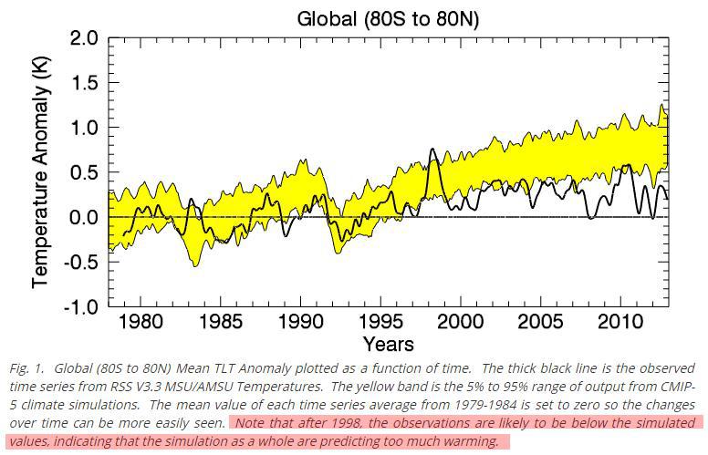
Regarding LWIRs ability to heat the ocean, I am often struck by how black and white the argument usually goes; as in…”LWIR cannot warm the oceans”. The counter argument goes, “can to”. I watched a very long post at WUWT go on and on like that. I tried once or twice to say wait a minute guys, let quantify this, or admit we don’t know. In general I think most of the energy of LWIR goes into evaporation, convection, and energy release through condensing at altitude, and radiation lost to space. However I can see the potential for the surface in some areas to warm, and slow the release of ocean heat. But if the state of our climate science is such that we do not know the answer to this in detail, then this alone, ignoring a dozen other major unknowns, is, IMV, adequate to completely discount the models.

Ron C. responds:

David, I am stimulated by this discussion and am posting it separately for others’ interest.

Your point about SH summer provides observational confirmation of the effects of thermal storage in the oceans.

Previously I have thought about your points in terms of the delay in heat transport from surface to space. Surrounded by the nearly absolute cold of space, our planet’s heat must move in that direction, which involves pushing it through the atmosphere. Of course, you are right that there is an additional delay within the oceans from the overturning required to bring energy to the surface for cooling. I like the image above depicting the water wheel as a massive traffic circle.

The Difference between climate on the Earth and the Moon

The intensity of solar energy is the same for the Earth and Moon, yet the dark side of the earth is much warmer than the dark side of the moon. And the bright side of the earth is much cooler than the bright side of the moon. Why are the two climates so different?

Earth’s oceans and atmosphere make the difference. Incoming sunlight is reduced by gases able to absorb IR and also by reflection from clouds and non-black surfaces. The earth’s surface is heated by sunlight, much of it stored and distributed by the oceans (71% of the planet surface). The atmosphere delays the upward passage of heat, and like a blanket slows the cooling allowing a buildup of temperature at the surface until there is a balance of heat radiating to space from the sky to match the solar energy coming in.

How the Atmosphere Processes Heat

There are 3 ways that heat (Infra-Red or IR radiation) passes from the surface to space.

1) A small amount of the radiation leaves directly, because all gases in our air are transparent to IR of 10-14 microns (sometimes called the “atmospheric window.” This pathway moves at the speed of light, so no delay of cooling occurs.

2) Some radiation is absorbed and re-emitted by IR active gases up to the tropopause. Calculations of the free mean path for CO2 show that energy passes from surface to tropopause in less than 5 milliseconds. This is almost speed of light, so delay is negligible.

3) The bulk gases of the atmosphere, O2 and N2, are warmed by conduction and convection from the surface. They also gain energy by collisions with IR active gases, some of that IR coming from the surface, and some absorbed directly from the sun. Latent heat from water is also added to the bulk gases. O2 and N2 are slow to shed this heat, and indeed must pass it back to IR active gases at the top of the troposphere for radiation into space.

In a parcel of air each molecule of CO2 is surrounded by 2500 other molecules, mostly O2 and N2. In the lower atmosphere, the air is dense and CO2 molecules energized by IR lose it to surrounding gases, slightly warming the entire parcel. Higher in the atmosphere, the air is thinner, and CO2 molecules can emit IR and lose energy relative to surrounding gases, who replace the energy lost.

This third pathway has a significant delay of cooling, and is the reason for our mild surface temperature, averaging about 15C. Yes, earth’s atmosphere produces a buildup of heat at the surface. The bulk gases, O2 and N2, trap heat near the surface, while IR-active gases, mainly H20 and CO2, provide the radiative cooling at the top of the atmosphere.

planetary-cooling-vents_full2

Understanding How Oceans Have Driven Climate Change

A syllabus from Dr. Bernaerts
(Reformatted, illustrated and lightly edited from his comment.)

Thanks for your interest. Let me first briefly outline the main parameters followed by an outline on the two major climatic changes since 1850.

As effective as the wind by ploughing through the sea.

The main parameters:

• At about 1850 the Little Ice Age ended and screw driven vessels entered the scene.

• Commercial motor ships churn-around a sea surface layer down to 15 meters depths, over a distance of 500 to 1000km during a day at sea,

• This results in a large exchange of warmer to colder water and vice versa.

• Any downward exchange happens immediately, and becomes part of the internal structure (heat and salinity). Any interaction between sea surface and the atmosphere happens only under certain (complex) conditions.

• The net impact is that the oceans presumably take in more heat as it is released again quickly.

• 160 years shipping and other ocean uses may have significantly contributed to global warming since 1850 (for example over the nighttime and winter seasons).

• As very little (at best) is known about these processes, the two major climatic changes provide helpful clues.

Main aspects of the two climatic changes, 1918/19-1939 & 1939/40 to mid-1970s.

Warming Period 1918/19-1939
Arctic Warming at the end of First World War is discussed in a book 2009 (p.106) at http://www.arctic-heats-up.com/

Winter temperatures exploded at Svalbard, and subsequently in the Atlantic sector of the Arctic Ocean, warming the Northern Hemisphere until WWII (USA until about 1933, Europe until 1939).The cause was likely a significant shift in the water structure (before and behind the Fram Strait), due to enormous naval activities around Great Britain that changed the heat and salinity structure of water masses from west of GB to the North Sea that all flows north. Naval war is the likely main contributor of this warming.


Global cooling 1939/40 to mid-1970s has two principle dimensions:

A.The three extreme war winters in Europe were the coldest for one hundred years. See my latest book (2012) http://www.seaclimate.com/

I discuss this event over about 175 pages (from a total of 220 pages), as each winter has specific features, as well with regard to naval activities. Europe’s sea areas (including the North and Baltic Sea) have stored a maximum heat by the end of August, which is usually released until end of March. Stirring hot coffee will cool it down; so will 1000 naval ships and other war activities at sea. Cold air from Siberia can take reign. That is anthropogenic climate change purely based on a large scale experiment with climate. It is evident naval actions caused these three extreme winters.

B. The North Atlantic and the West-Pacific became a major naval battle ground after Pearl Harbor in December 1941. Operations penetrated the sea surface layer down to depths of 200 meters, not to mention ships, and airplanes sunk, and the many million shells fired. Global cooling was established for three decades, because several years’ war at sea generated a huge chaos in a very complex water structure (heat & salinity), which needed more than three decades to ‘recover’.

Summary

The three extreme winters in Europe “tell it all”. Climate sciences had seven decades time to analyze the ‘large scale field experiment”. A thorough understanding would definitely establish that naval war activities was the major cause, which subsequently would inevitable require to investigate the Arctic warming and global cooling as a naval war related matter (to a very noticeable degree) as well. Actually, understanding “Climate as the continuation of the oceans by other means” would have raised an alert more than one century ago that screw driven vessels and other human activities at sea may change the sea in a way that alters weather and climate.

A good place to start is chapter A3 “Man-made climate –since 1850” at: http://www.seaclimate.com/a/a3.html

Ron; I hope the brief text provides enough aspects concerning the subject. Your further kind assistance to get the message across would be highly appreciated. Thanks a lot, Arnd.

No, Thank you, Dr. Bernaerts.

Climate Report from the Water World

In 1995 many people saw the cli-sci-fi (Climate Science Fiction) thriller based on polar ice melting and all land surface covered with water.

But that hypothetical world is not the subject of this post, rather it is our very own planet earth just as it is today.

We humans, parochial as we are, imagine the earth’s surface to be land because that is where we live. In fact, the earth’s surface is 71% water, and the Northern Hemisphere (NH) consists of 30% water and 20% land, while the SH is a whopping 41% water and only 9% land. I was reminded of this fact recently while looking at Australian temperature records. The image below shows the effect of living on a piece of land upon a water world.

“Warming over Australia has been consistent with warming in the surrounding oceans.”

Indeed, how could it be otherwise for an island continent surrounded by water? The graph above shows a gentle rising of sea surface temperatures (SST) following the end of the Little Ice Age, overlaid with various ocean shifts (ENSO, AMO, NAO, etc.). Since 84% of Australians live within 50 km of the coast, and weather stations tend to be located where people live, it’s not surprising that the land surface temperature records mimic the sea surface variations.

But the effect is not limited to Australia. Climate research centers estimate global mean surface temperatures weighted according to grids, so those metrics are dominated by the ocean SSTs. 2014 was warm because of the mild undeclared El Nino, which persists today and gives hope to those wanting a record warm year in 2015.

But this is not about CO2. It has everything to do with water heated by shortwave solar radiation, stored and circulating in complex patterns, driven by the temperature differential between the equator and the poles. Scientists are gaining insight into the temperature dynamics of our water world.

The Pacific Makes Waves Worldwide

Among the oceans, the Pacific is the gorilla whose fluctuations drive changes across the water world. Short-term ENSO events ripple globally, and in the longer-term, there are effects from the Interdecadal Pacific Oscillation (IPO), not to be confused with an Initial Public Offering. Here are some recent research findings:

“From 1920 to 2012, there are roughly two warm IPO phases (1924–1945 and 1977–1998, with warm SSTs in the central and eastern tropical Pacific) and two cold IPO phases (1946–1976 and 1999–2012, with cold SSTs in the same region). The most recent cold IPO phase is still continuing. We found that phase switches of the IPO are concurrent with major climate transitions over the globe, including abrupt shifts in SST, SLP, T and P.”

“Annual surface air temperature is positively correlated with the IPO index (i.e., higher T during warming IPO phases such as 1924–1945 and 1977–1998) over western North America except its Southwest, mid-latitude central and eastern Asia, and central and northern Australia, but the correlation is negative over northeastern North America, northeastern South America, southeastern Europe, and northern India. Annual precipitation tends to be higher (lower) during warm (cold) IPO phases such as 1924–1945 and 1977–1998 (1946–1976 and 1999–2012) over southwestern North America, northern India, and central Argentina, while it is the opposite over the maritime continent including much of Australia, southern Africa, and northeastern Asia (Fig. 4b).”

“Besides the direct impacts on decadal variations in T and P, we also found some decadal modulations of ENSO’s influence on T and P on multi-year timescales by the IPO over northeastern Australia, northern India, southern Africa and western Canada.”

“Thus, the IPO is an ENSO-like low-frequency mode not just in its SST and SLP patterns (Zhang et al. 1997), but also in its impacts on T and P and atmospheric fields. These results imply that many of the surface and atmospheric processes associated with ENSO also apply to the IPO phase changes, with the warm (cold) IPO phase resembling El Nino (La Nina). Our results also suggest that it is important to predict IPO’s phase change for decadal climate predictions.”

From: The influence of the Interdecadal Pacific Oscillation on Temperature and Precipitation over the Globe Bo Dong • Aiguo Dai 2015 http://www.cgd.ucar.edu/cas/adai/papers/DongDai-CD2015-IPO.pdf

So let’s see how those warming and cooling periods show up in the SST historical records. HadSST3 dataset is available here:
http://www.metoffice.gov.uk/hadobs/hadsst3/data/download.html

I analyzed the annual global record and got the following results:

HadSST3 Global Temperature Anomaly Trends

1924-1945 0.171 C/decade
1945-1977 -0.028 C/decade
1977-1998 0.150 C/decade
1998-2014 0.054 C/decade
1924-2014 0.057 C/decade

If those trends look familiar, it’s because you see the same pattern in any of the global surface temperature datasets.

Conclusion:

Living on our water world means our temperatures and precipitation fluctuate according to ocean circulations and oscillations, especially ENSO and IPO patterns in the Pacific basin.

Climate is the continuation of oceans by other means. Dr. Arnd Bernaerts

Note:

I think SSTs are a reasonable proxy for natural variability over the last century or so. The long-term trend is 0.5C/century with multi-decadal periods as high as +1.7C/century, and as low as -0.3C/century. The latter one was enough to cause an ice age scare.

In advance of COP Paris, some want to project warming of +1.5C as requiring action. We’ve been there twice already recently, and much warmer still in the distant past.

Climate Thinking Out of the Box

CMIP5 vs RSS

It seems that climate modelers are dealing with a quandary: How can we improve on the unsatisfactory results from climate modeling?

Shall we:
A.Continue tweaking models using classical maths though they depend on climate being in quasi-equilibrium; or,
B.Start over from scratch applying non-equilibrium maths to the turbulent climate, though this branch of math is immature with limited expertise.

In other words, we are confident in classical maths, but does climate have features that disqualify it from their application? We are confident that non-equilibrium maths were developed for systems such as the climate, but are these maths robust enough to deal with such a complex reality?

It appears that some modelers are coming to grips with the turbulent quality of climate due to convection dominating heat transfer in the lower troposphere. Heretofore, models put in a parameter for energy loss through convection, and proceeded to model the system as a purely radiative dissipative system. Recently, it seems that some modelers are striking out in a new, possibly more fruitful direction. Herbert et al 2013 is one example exploring the paradigm of non-equilibrium steady states (NESS). Such attempts are open to criticism from a classical position, but may lead to a breakthrough for climate modeling.

That is my layman’s POV. Here is the issue stated by practitioners, more elegantly with bigger words:

“In particular, it is not obvious, as of today, whether it is more efficient to approach the problem of constructing a theory of climate dynamics starting from the framework of hamiltonian mechanics and quasi-equilibrium statistical mechanics or taking the point of view of dissipative chaotic dynamical systems, and of non-equilibrium statistical mechanics, and even the authors of this review disagree. The former approach can rely on much more powerful mathematical tools, while the latter is more realistic and epistemologically more correct, because, obviously, the climate is, indeed, a non-equilibrium system.”

Lucarini et al 2014

Click to access 1311.1190.pdf

Here’s how Herbert et al address the issue of a turbulent, non-equilibrium atmosphere. Their results show that convection rules in the lower troposphere and direct warming from CO2 is quite modest, much less than current models project.

“Like any fluid heated from below, the atmosphere is subject to vertical instability which triggers convection. Convection occurs on small time and space scales, which makes it a challenging feature to include in climate models. Usually sub-grid parameterizations are required. Here, we develop an alternative view based on a global thermodynamic variational principle. We compute convective flux profiles and temperature profiles at steady-state in an implicit way, by maximizing the associated entropy production rate. Two settings are examined, corresponding respectively to the idealized case of a gray atmosphere, and a realistic case based on a Net Exchange Formulation radiative scheme. In the second case, we are also able to discuss the effect of variations of the atmospheric composition, like a doubling of the carbon dioxide concentration.

The response of the surface temperature to the variation of the carbon dioxide concentration — usually called climate sensitivity — ranges from 0.24 K (for the sub-arctic winter profile) to 0.66 K (for the tropical profile), as shown in table 3. To compare these values with the literature, we need to be careful about the feedbacks included in the model we wish to compare to. Indeed, if the overall climate sensitivity is still a subject of debate, this is mainly due to poorly understood feedbacks, like the cloud feedback (Stephens 2005), which are not accounted for in the present study.”

Abstract from:
Vertical Temperature Profiles at Maximum Entropy Production with a Net Exchange Radiative Formulation
Herbert et al 2013

Click to access 1301.1550.pdf

In this modeling paradigm, we have to move from a linear radiative Energy Budget to a dynamic steady state Entropy Budget. As Ozawa et al explains, this is a shift from current modeling practices, but is based on concepts going back to Carnot.

“Entropy of a system is defined as a summation of “heat supplied” divided by its “temperature” [Clausius, 1865].. Heat can be supplied by conduction, by convection, or by radiation. The entropy of the system will increase by equation (1) no matter which way we may choose. When we extract the heat from the system, the entropy of the system will decrease by the same amount. Thus the entropy of a diabatic system, which exchanges heat with its surrounding system, can either increase or decrease, depending on the direction of the heat exchange. This is not a violation of the second law of thermodynamics since the entropy increase in the surrounding system is larger.

Carnot regarded the Earth as a sort of heat engine, in which a fluid like the atmosphere acts as working substance transporting heat from hot to cold places, thereby producing the kinetic energy of the fluid itself. His general conclusion about heat engines is that there is a certain limit for the conversion rate of the heat energy into the kinetic energy and that this limit is inevitable for any natural systems including, among others, the Earth’s atmosphere.

Thus there is a flow of energy from the hot Sun to cold space through the Earth. In the Earth’s system the energy is transported from the warm equatorial region to the cool polar regions by the atmosphere and oceans. Then, according to Carnot, a part of the heat energy is converted into the potential energy which is the source of the kinetic energy of the atmosphere and oceans.

Thus it is likely that the global climate system is regulated at a state with a maximum rate of entropy production by the turbulent heat transport, regardless of the entropy production by the absorption of solar radiation This result is also consistent with a conjecture that entropy of a whole system connected through a nonlinear system will increase along a path of evolution, with a maximum rate of entropy production among a manifold of possible paths [Sawada, 1981]. We shall resolve this radiation problem in this paper by providing a complete view of dissipation processes in the climate system in the framework of an entropy budget for the globe.

The hypothesis of the maximum entropy production (MEP) thus far seems to have been dismissed by some as coincidence. The fact that the Earths climate system transports heat to the same extent as a system in a MEP state does not prove that the Earths climate system is necessarily seeking such a state. However, the coincidence argument has become harder to sustain now that Lorenz et al. [2001] have shown that the same condition can reproduce the observed distributions of temperatures and meridional heat fluxes in the atmospheres of Mars and Titan, two celestial bodies with atmospheric conditions and radiative settings very different from those of the Earth.”

THE SECOND LAW OF THERMODYNAMICS AND THE GLOBAL CLIMATE SYSTEM: A REVIEW OF THE MAXIMUM ENTROPY PRODUCTION PRINCIPLE
Hisashi Ozawa et al 2003

Click to access Ozawa.pdf

Lawrence Lab Report: Proof of Global Warming?

It’s important to deconstruct this study because it is touted in the press as silencing “Climate Deniers” and as giving scientific proof of the greenhouse gas effect, once and for all. For example, a CBC article said this:

“A recent experiment at the Lawrence Berkeley National Laboratory in California has directly measured the warming effect of our carbon emissions, using data from instruments that measure the infrared radiation being reflected back to the ground by the atmosphere – the so-called greenhouse effect.
They found that the amount of radiation coming down increased between 2000 and 2010 in step with the rise of carbon dioxide in the atmosphere. So, the effect is real. And since we are continuing to increase our carbon emissions, change will continue to happen, like it or not, both warm and cold.”

The media was agog over this paper, saying that it measures the warming effect of CO2 in the atmosphere, and is proof of the greenhouse gas effect.

This paper claims to prove rising CO2 in the atmosphere increases down-welling infra-red radiation (DWIR), thereby warming the earth’s surface. The claim is based on observations from 2 sites, in Alaska and Oklahoma. Let’s examine the case made.

Observation: In Alaska and Oklahoma CO2 and DWIR are both increasing.
Claim: Additional CO2 is due to fossil fuel emissions.
Claim: Higher DWIR is due to higher CO2 levels.
Claim: Global DWIR is rising.
Claim: Global surface temperatures are rising.
LL Conclusion: Fossil fuel emissions are causing Global surface temperatures to rise

There are several issues that undermine the report’s conclusion.

Issue: What is the source of rising CO2?
Response: Natural sources of CO2 overwhelm human sources.

The sawtooth pattern of seasonal CO2 concentrations is consistent with release of CO2 from the oceans. Peaks are in March when SH oceans are warmest (60% of world oceans), and valleys are in September when NH oceans are warmest. In contrast biosphere activities peak in January in SH and July in NH.

CO2 content of the oceans is 50 times that of the atmosphere, resulting in the sawtooth extremes. Human emissions are ~5 to 7 Gigatons compared to ~150 Gigatons from natural sources.

Issue: What is the effect of H2O and CO2 on DWIR?
Response: H2O provides 90% of IR activity in the atmosphere.

The long term increase in DWIR can be explained by increasing cloudiness, deriving from evaporation when the sunlight heats the oceans. A slight change in H2O vapor overwhelms the effect of CO2 activity, and H2O varies greatly from place to place, while the global average is fairly constant.

Issue: What is the global trend of DWIR?
Response: According CERES satellites, DWIR has decreased globally since 2000, resulting in an increasing net IR loss upward from the surface.

Globally, Earth’s surface has strongly strengthened its ability to cool radiatively from 2000 to 2014 (by about 1.5 W/m2 or ~1 W/m2 per decade) according to CERES. The increased upward heat loss from the surface is matched by decreasing trend of DWIR globally. And this is in spite of significantly increasing atmospheric content of both CO2 and H2O (WV & clouds) + allegedly rising temps since 2000.

Conclusion:
The rise in CO2 is almost all from natural sources, not fossil fuel emissions.
IR activity is almost all from H2O, not from CO2.
Global DWIR is lower this century, and the surface heat loss is less impeded than before.
Global surface temperatures are not rising with rising fossil fuel emissions.

In fact, you need only apply a little critical intelligence to this paper, and it falls like a house of cards. Are there no journalists with thinking caps allowed to write about this stuff?

The Permafrost Bogeyman

The permafrost Methane bogeyman disappears in the light of the facts.

1) When there was warming in places like Alaska, atmospheric methane did not increase.

2) Permafrost depletion in the NH stopped since 2005.

3) When permafrost thaws, vegetation grows and removes more CO2 than is released by the melting. The region acts as a sink, not a source of CO2.

4) Past warm periods (Medieval and Holocene warmings) did not produce increases in methane.

So scientists with models are stirring up alarm about thawing of Siberian permafrost. But there are scientists in Siberia monitoring the situation. What do they say?

“Indeed above at the surface it has gotten warmer, but that’s just part of a normal cycle. The permafrost is rock hard, And that is how it is going to stay. There’s no talk of thawing.” Michali Grigoryev
http://notrickszone.com/2012/11/19/russian-arctic-scientist-permafrost-changes-due-to-natural-factors-its-going-to-be-colder/

“It seems that the permafrost should be melting if the temperature is rising. However, many areas are witnessing the opposite. The average annual temperature is getting higher, but the permafrost remains and has even started to spread. Why? An important factor is the snow cover. Global warming reduces it, therefore making the heat insulator for the permafrost thinner. Then even weak frosts are enough to freeze the ground deeper below the surface.”

Nikolai Osokin is a glaciologist at the Institute of Geography, the Russian Academy of Sciences.

http://en.rian.ru/analysis/20070323/62485608.html
“The Russian Academy of Sciences has found that the annual temperature of soils (with seasonable variations) has been remaining stable despite the increased average annual air temperature caused by climate change. If anything, the depth of seasonal melting has decreased slightly.”

“This is just another scare story . . . This ecological structure is balanced and is not about to harm people with gas discharges.”
Vladimir Melnikov is the director of the world’s only Institute of the Earth’s Cryosphere. The Russian Academy of Sciences’ Institute is located in the Siberian city of Tyumen and investigates the ways in which ground water becomes ice and permafrost.

“The boundaries of the Russian permafrost zone remain virtually unchanged. At the same time, the permafrost is several hundred meters deep. For methane, other gases and hydrates to escape to the surface, it would have to melt at tremendous depths, which is impossible.”
Yuri Izrael, director of the Institute of Climatology and Ecology of the Russian Academy of Sciences.

http://en.rian.ru/analysis/20050822/41201605-print.html

Runaway warming from permafrost thawing has not happened before, is not happening now, but we should believe it will happen if we don’t do something?