The complaint, filed Thursday in the U.S. District Court in Montana, challenges three executive orders: “Unleashing American Energy,” “Declaring a National Energy Emergency” and “Reinvigorating America’s Beautiful Clean Coal Industry.” The lawsuit argues that with the orders, the Trump administration knowingly is advancing an agenda that will increase greenhouse gas pollution that already is stressing the global climate to a dangerous extent.
The litigation argues the situation infringes on the young people’s constitutional rights to life and liberty, as well as falling afoul of other laws approved by Congress that protect public health and the environment. The plaintiffs want the court to declare the executive orders unconstitutional, block their implementation and reaffirm the legal limits on presidential power.
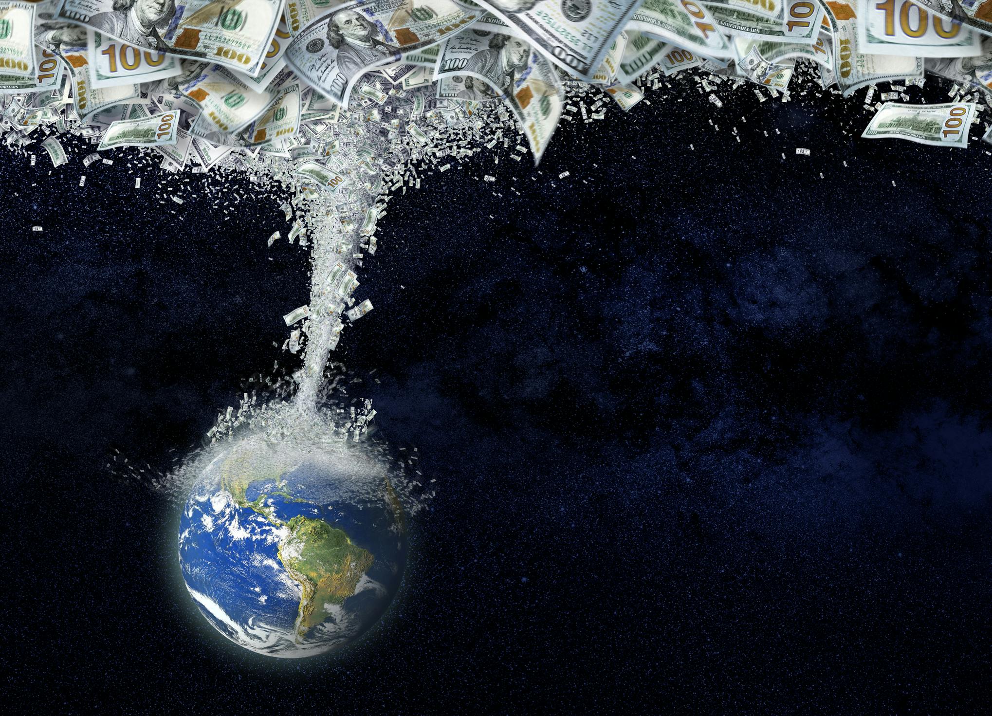
“From day one of the current administration, President Trump has issued directives to increase fossil fuel use and production and block an energy transition to wind, solar, battery storage, energy efficiency, and electric vehicles (“EVs”),” the lawsuit states. “President Trump’s EOs falsely claim an energy emergency, while the true emergency is that fossil fuel pollution is destroying the foundation of Plaintiffs’ lives.”

It’s the same argument from the same people (Our Children’s Trust) that was shot down in flames just a year ago. There were multiple attempts to undo the damaged legal maneuver to no avail. Below is why this latest litigation should be put out of its misery at once.
Appeals Court Rules Against Kids’ Climate Lawsuit, May 1, 2024
Ninth Circuit Court of Appeals grants Federal government’s petition for writ of mandamus in the case of Juliana v. United States, originally filed in 2015. Ruling excerpts are below in italics with my bolds. 20240501_docket-24-684_order
In the underlying case, twenty-one plaintiffs (the Juliana plaintiffs) claim that—by failing to adequately respond to the threat of climate change—the government has violated a putative “right to a stable climate system that can sustain human life.” Juliana v. United States, No. 6:15-CV-01517-AA, 2023 WL 9023339, at *1 (D. Or. Dec. 29, 2023). In a prior appeal, we held that the Juliana plaintiffs lack Article III standing to bring such a claim. Juliana v. United States, 947 F.3d 1159, 1175 (9th Cir. 2020). We remanded with instructions to dismiss on that basis. Id. The district court nevertheless allowed amendment, and the government again moved to dismiss. The district court denied that motion, and the government petitioned for mandamus seeking to enforce our earlier mandate. We have jurisdiction to consider the petition. See 28 U.S.C. § 1651. We grant it.
In the prior appeal, we held that declaratory relief was “not substantially likely to mitigate the plaintiffs’ asserted concrete injuries.” Juliana, 947 F.3d at 1170. To the contrary, it would do nothing “absent further court action,” which we held was unavailable. Id. We then clearly explained that Article III courts could not “step into the shoes” of the political branches to provide the relief the Juliana plaintiffs sought. Id. at 1175. Because neither the request for declaratory relief nor the request for injunctive relief was justiciable, we “remand[ed] th[e] case to the district court with instructions to dismiss for lack of Article III standing.” Id. Our mandate was to dismiss.
The district court gave two reasons for allowing amendment. First, it concluded that amendment was not expressly precluded. Second, it held that intervening authority compelled a different result. We reject each.
The first reason fails because we “remand[ed] . . . with instructions to dismiss for lack of Article III standing.” Id. Neither the mandate’s letter nor its spirit left room for amendment. See Pit River Tribe, 615 F.3d at 1079.
The second reason the district court identified was that, in its view, there was an intervening change in the law. District courts are not bound by a mandate when a subsequently decided case changes the law. In re Molasky, 843 F.3d 1179, 1184 n.5 (9th Cir. 2016). The case the court identified was Uzuegbunam v. Preczewski, which “ask[ed] whether an award of nominal damages by itself can redress a past injury.” 141 S. Ct. 792, 796 (2021). Thus, Uzuegbunam was a damages case which says nothing about the redressability of declaratory judgments. Damages are a form of retrospective relief. Buckhannon Bd. & Care Home v. W. Va. Dep’t of Health & Human Res., 532 U.S. 598, 608–09 (2001). Declaratory relief is prospective. The Juliana plaintiffs do not seek damages but seek only prospective relief. Nothing in Uzuegbunam changed the law with respect to prospective relief.
We held that the Juliana plaintiffs lack standing to bring their claims and told the district court to dismiss. Uzuegbunam did not change that. The district court is instructed to dismiss the case forthwith for lack of Article III standing, without leave to amend.
Background July 2023: Finally, a Legal Rebuttal on the Merits of Kids’ Climate Lawsuit
As reported last month, the Oregon activist judge invited the plaintiffs in Juliana vs US to reopen that case even after the Ninth Circuit shot it down. Now we have a complete and thorough Motion from the defendant (US government) to dismiss this newest amended complaint. Most interesting is the section under the heading starting on page 30. Excerpts in italics with my bolds and added images.
Plaintiffs’ Claims Fail on the Merits
Because Plaintiffs’ action fails at the jurisdictional threshold, the Ninth Circuit never reached—and this Court need not reach—the merits of the claims. . . Plaintiffs’ second amended complaint, which supersedes the first amended complaint, asserts the same claims that were brought in the first amended complaint, which this Court addressed in orders that the Ninth Circuit reversed. Defendants thus renew their objection that Plaintiffs’ claims fail on the merits and should be dismissed pursuant to Fed. R. Civ. P. 12(b)(6).
A. There is no constitutional right to a stable climate system.
The Supreme Court has repeatedly instructed courts considering novel due process claims
to “‘exercise the utmost care whenever . . . asked to break new ground in this field,’… lest the liberty protected by the Due Process Clause be subtly transformed” into judicial policy preferences. More specifically, the Supreme Court has “regularly observed that the Due Process Clause specially protects those fundamental rights and liberties which are, objectively, ‘deeply rooted in this Nation’s history and tradition.’” Plaintiffs’ request that this Court recognize an implied fundamental right to a stable climate system contradicts that directive, because such a purported right is without basis in the Nation’s history or tradition.
The proposed right to a “stable climate system” is nothing like any fundamental right ever recognized by the Supreme Court. The state of the climate is a public and generalized issue, and so interests in the climate are unlike the particularized personal liberty or personal privacy interests of individuals the Supreme Court has previously recognized as being protected by fundamental rights. “[W]henever federal courts have faced assertions of fundamental rights to a ‘healthful environment’ or to freedom from harmful contaminants, they have invariably rejected those claims.”. Plaintiffs’ First Claim for Relief must be dismissed.

B. Plaintiffs fail to allege a cognizable state-created danger claim.
The First Claim for Relief must also be dismissed because the Constitution does not impose an affirmative duty to protect individuals, and Plaintiffs have failed to allege a cognizable claim under the “state-created danger” exception to that rule.
As a general matter:
[The Due Process Clause] is phrased as a limitation on the State’s power to act, not as a guarantee of certain minimal levels of safety and security. It forbids the State itself to deprive individuals of life, liberty, or property without “due process of law,” but its language cannot fairly be extended to impose an affirmative obligation on the State to ensure that those interests do not come to harm through other means.
Thus, the Due Process Clause imposes no duty on the government to protect persons from harm inflicted by third parties that would violate due process if inflicted by the government.
Plaintiffs contend that the government’s “deliberate actions” and “deliberate indifference” with regard to the dangers of climate change amount to a due process violation under the state-created danger exception.
First, Plaintiffs have identified no harms to their “personal security or bodily integrity” of the kind and immediacy that qualify for the state-created danger exception. . . But here, Plaintiffs allege that general degradation of the global climate has harmed their “dignity, including their capacity to provide for their basic human needs, safely raise families, practice their religious and spiritual beliefs, [and] maintain their bodily integrity” and has prevented them from “lead[ing] lives with access to clean air, water, shelter, and food.” Those types of harm are unlike the immediate, direct, physical, and personal harms at issue in the above-cited cases.
Second, Plaintiffs identify no specific government actions—much less government actors—that put them in such danger. Instead, Plaintiffs contend that a number of (mostly unspecified) agency actions and inactions spanning the last several decades have exposed them to harm. This allegation of slowly-recognized, long-incubating, and generalized harm by itself conclusively distinguishes their claim from all other state-created danger cases recognized by the Ninth Circuit.
Third, Plaintiffs do not allege that government actions endangered Plaintiffs in particular. . . As explained above, Plaintiffs’ asserted injuries arise from a diffuse, global phenomenon that affects every other person in their communities, in the United States, and throughout the world.
For all these reasons, there is no basis for finding a violation of Plaintiffs’ due process right under the state-created danger doctrine, and Plaintiffs’ corresponding claim must be dismissed.
C. No federal public trust doctrine creates a right to a stable climate system.
Plaintiffs’ Fourth Claim for Relief, asserting public trust claims, should be dismissed for two independent reasons. First, any public trust doctrine is a creature of state law that applies narrowly and exclusively to particular types of state-owned property not at issue here. That doctrine has no application to federal property, the use and management of which is entrusted exclusively to Congress. . .Consequently, there is no basis for Plaintiffs’ public trust claim against the federal government under federal law.
Second, the “climate system” or atmosphere is not within any conceivable federal public trust.
1. No public trust doctrine binds the federal government.
Plaintiffs rely on an asserted public trust doctrine for the proposition that the federal government must “take affirmative steps to protect” “our country’s life-sustaining climate system,” which they assert the government holds in trust for their benefit. But because any public trust doctrine is a matter of state law only, public trust claims may not be asserted against the federal government under federal law. . . The Supreme Court has without exception treated public trust doctrine as a matter of state law with no basis in the United States Constitution.
2. Any public trust doctrine would not apply to the “climate system” or the atmosphere.
Independently, any asserted public trust doctrine does not help Plaintiffs here. Public trust cases have historically involved state ownership of specific types of natural resources, usually limited to submerged and submersible lands, tidelands, and waterways. . . The climate system or atmosphere is unlike any resource previously deemed subject to a public trust. It cannot be owned and, due to its ephemeral nature, cannot remain within the jurisdiction of any single government. No court has held that the climate system or atmosphere is protected by a public trust doctrine. Indeed, the concept has been widely rejected.
For all these reasons, the Court should dismiss Plaintiffs’ Fourth Claim for Relief.

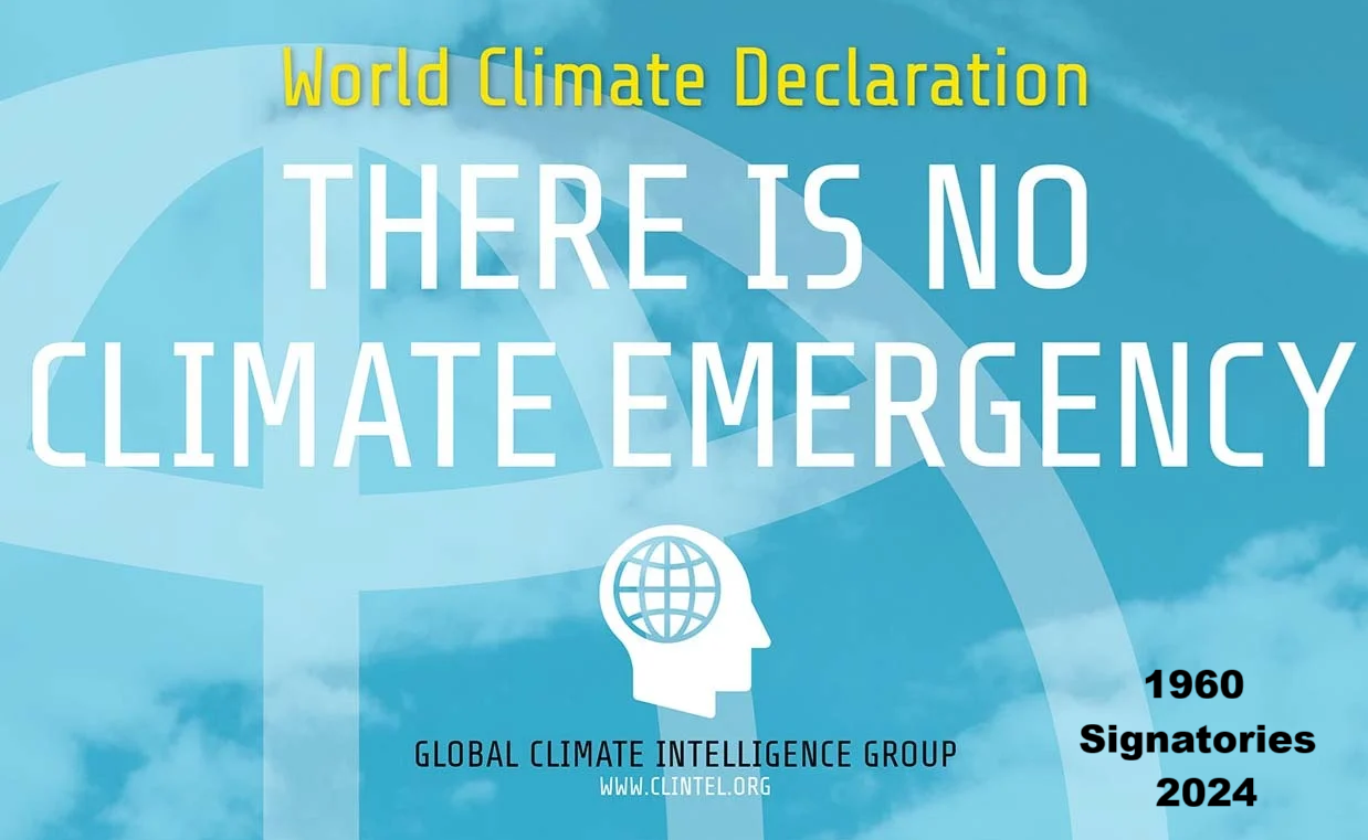
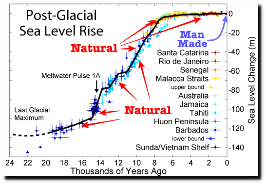
Background Post Update on Zombie Kids Climate Lawsuits: (Juliana vs. US) (Held vs Montana)

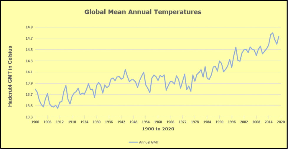
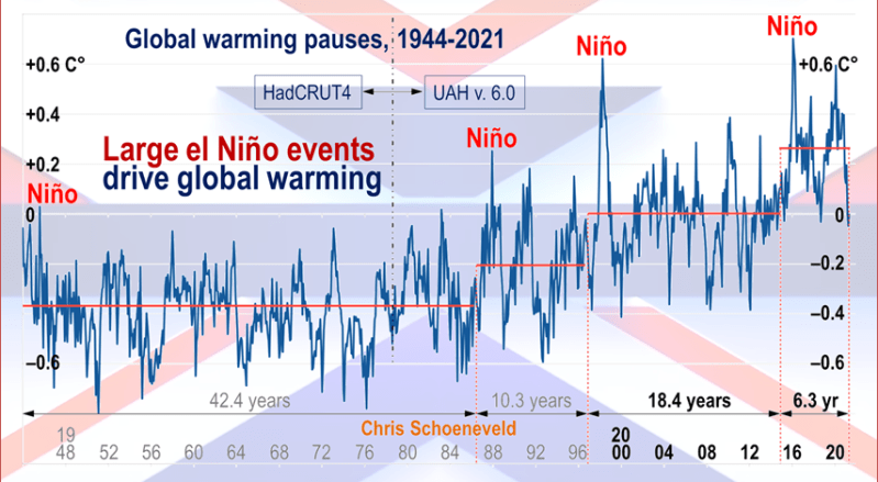
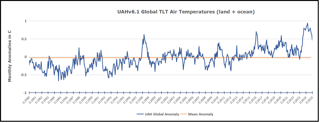
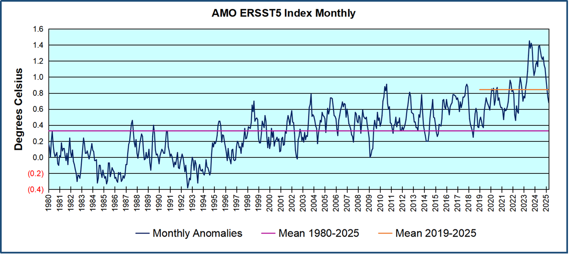
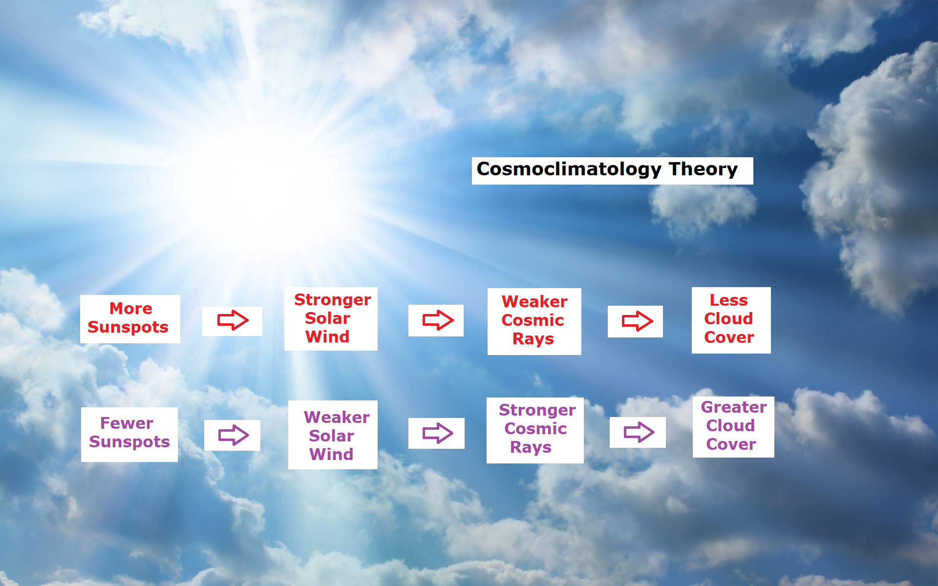
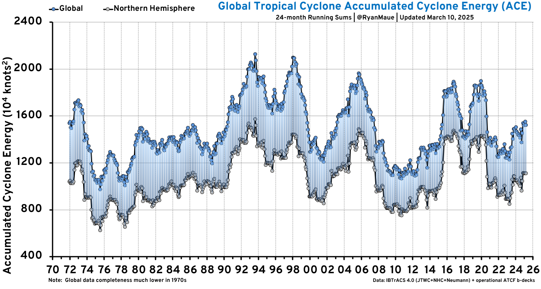
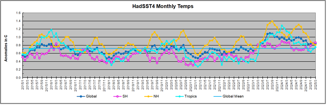
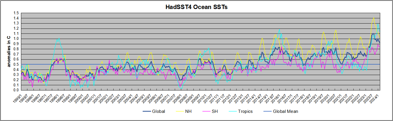
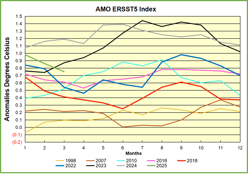
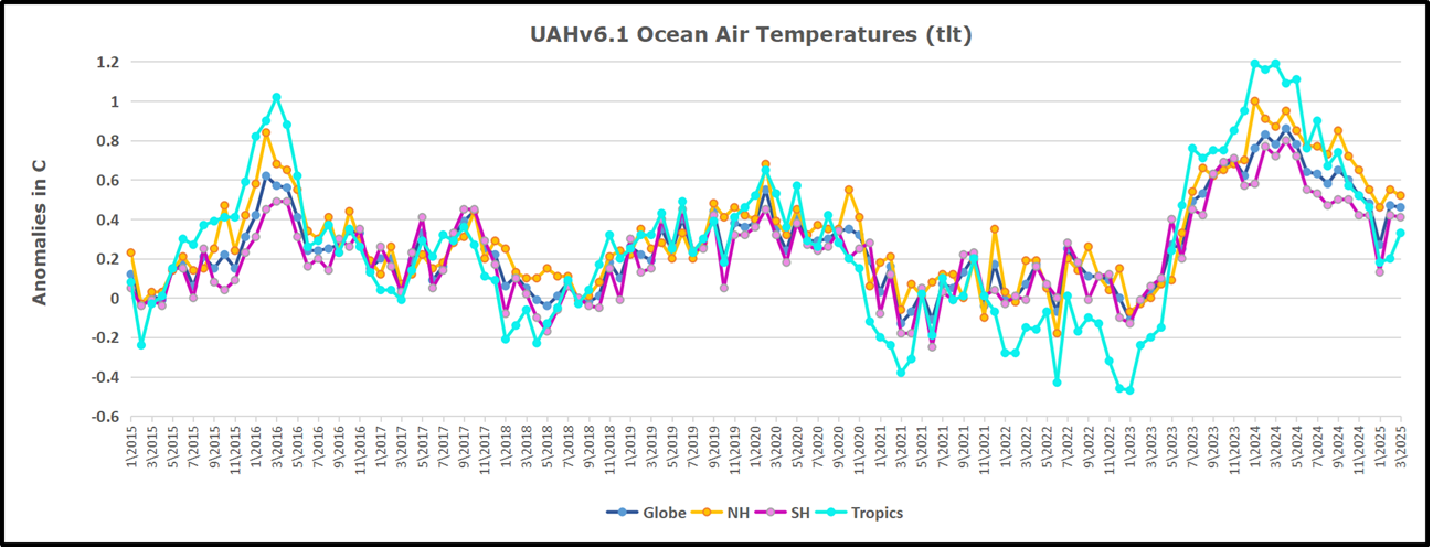
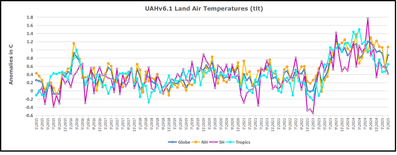
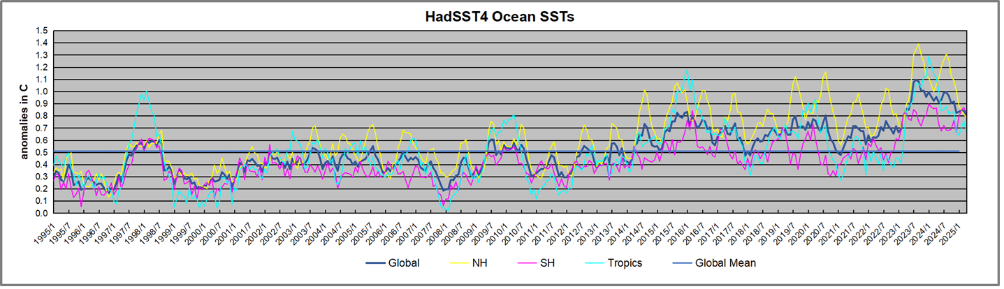
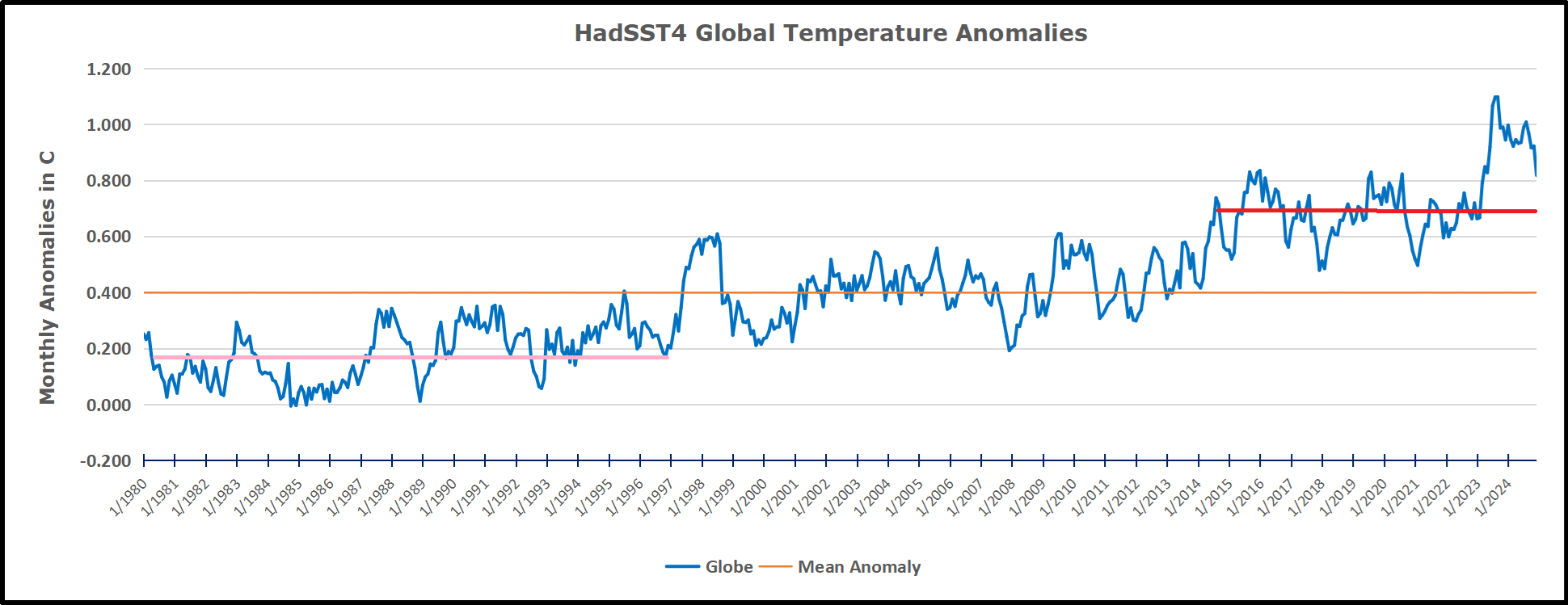
 The best context for understanding decadal temperature changes comes from the world’s sea surface temperatures (SST), for several reasons:
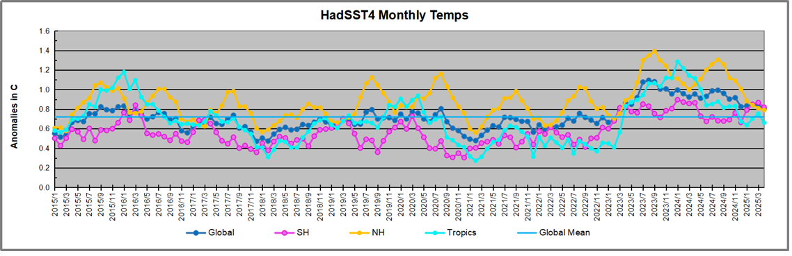


 The recently published paper is
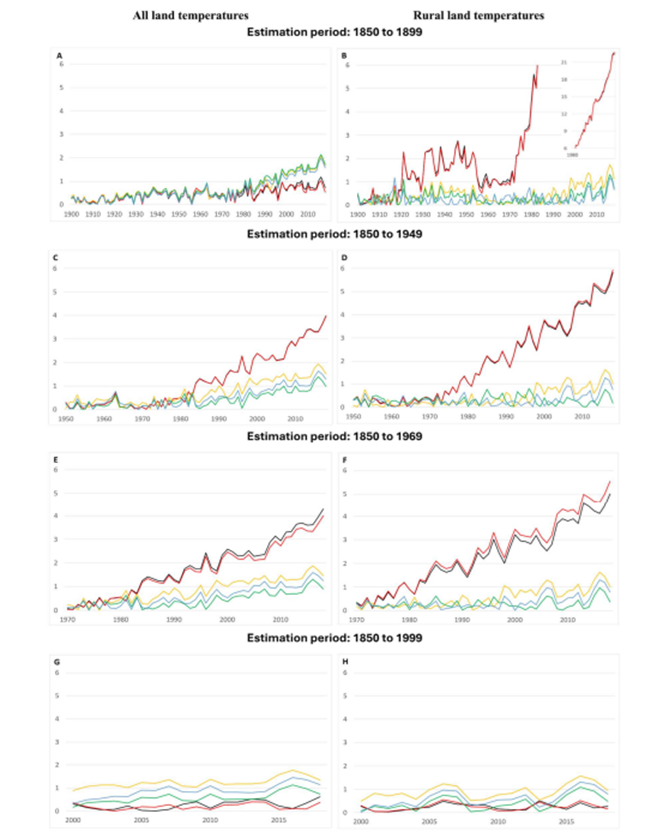
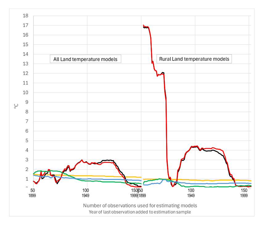
 The anthropogenic models’ unreliability would appear to void policy relevance. In practice, even the models validated in this study may fail to improve accuracy relative to naïve forecasts due to uncertainty over the future causal variable values. Our findings emphasize that out-of-sample forecast errors, not statistical fit, should be used to choose between models (hypotheses).
 In sum, the objective given to the IPCC researchers and the approach that they have taken suggests that plausible alternative hypotheses on the causes of terrestrial temperature changes may not have been adequately tested, as is required by the scientific method (Armstrong and Green, 2022). That concern is consistent with Armstrong and Green’s (2022) observation that government sponsorship of research can create incentives that may influence researchers’ choices of hypotheses to test and how they test them.
 1.5 Hypotheses tested