The recently published paper is Are Climate Model Forecasts Useful for Policy Making? by Kesten C. Green and Willie Soon. Excerpts in italics with my bolds and added images.
Effect of Variable Choice on Reliability and Predictive Validity
Abstract
For a model to be useful for policy decisions, statistical fit is insufficient. Evidence that the model provides out-of-estimation-sample forecasts that are more accurate and reliable than those from plausible alternative models, including a simple benchmark, is necessary.
The UN’s IPCC advises governments with forecasts of global average temperature drawn from models based on hypotheses of causality. Specifically, manmade warming principally from carbon dioxide emissions (Anthro) tempered by the effects of volcanic eruptions (Volcanic) and by variations in the Sun’s energy (Solar). Out-of-sample forecasts from that model, with and without the IPCC’s favoured measure of Solar, were compared with forecasts from models that excluded human influence and included Volcanic and one of two independent measures of Solar. The models were used to forecast Northern Hemisphere land temperatures and—to avoid urban heat island effects—rural only temperatures. Benchmark forecasts were obtained by extrapolating estimation sample median temperatures.
The independent solar models reduced forecast errors relative to those of the benchmark model for all eight combinations of four estimation periods and the two temperature variables tested. The models that included the IPCC’s Anthro variable reduced errors for only three of the eight combinations and produced extreme forecast errors from most model estimation periods. The correlation between estimation sample statistical fit and forecast accuracy was -0.26. Further tests might identify better models: Only one extrapolation model and only two of many possible independent solar models were tested, and combinations of forecasts from different methods were not examined.
 The anthropogenic models’ unreliability would appear to void policy relevance. In practice, even the models validated in this study may fail to improve accuracy relative to naïve forecasts due to uncertainty over the future causal variable values. Our findings emphasize that out-of-sample forecast errors, not statistical fit, should be used to choose between models (hypotheses).
Background
In their attempts to achieve the IPCC objective of identifying a human cause for temperature changes—specifically “global warming”—the IPCC researchers have framed the problem as one of “attributing” changes in the Earth’s temperature to the respective contributions of putative anthropogenic (“Anthro”) principally carbon dioxide emissions altering the composition of the atmosphere—and natural influences—principally aerosols from volcanic eruptions altering the composition of the atmosphere (“Volcanic”), and total solar irradiance, or TSI, variations (“Solar”).
Given the task they were set, the IPCC researchers have devoted
much of their efforts into developing estimates of the Anthro variable.
The IPCC’s most recent, AR6, report (IPCC, 2021) only considered one estimate of Solar for the purpose of attribution (Matthes et al., 2017) and made no allowance for the effect of urban heat islands on the temperature measures they used (Connolly et al., 2021, 2023; Soon et al., 2023). Moreover, a study of the statistical attribution or “fingerprinting” approach used by IPCC researchers (e.g., Allen and Tett, 1999; Hasselmann, et al., 1995; Hegerl et al., 1997; Santer et al.,1995) concluded that the approach was invalid (McKitrick, 2022). The IPCC authors’ analyses failed to meet the assumptions of the method they used, and they failed to correctly implement the method.
 In sum, the objective given to the IPCC researchers and the approach that they have taken suggests that plausible alternative hypotheses on the causes of terrestrial temperature changes may not have been adequately tested, as is required by the scientific method (Armstrong and Green, 2022). That concern is consistent with Armstrong and Green’s (2022) observation that government sponsorship of research can create incentives that may influence researchers’ choices of hypotheses to test and how they test them.
1.1 Alternative hypotheses on Solar
To address the first of the foregoing limitations in the IPCC attribution studies—failure to fairly test alternative TSI estimates—Connolly et al. (2021, 2023) comprehensively reviewed alternative estimates of TSI covering the 169 years from 1850 to 2018. In addition to the Matthes, et al. (2017) TSI estimates series used by the IPCC (2021)—henceforth “IPCC Solar”—Connolly et al. (2023) identified 27 alternative Solar time series.

The alternative estimates of Solar correlate quite well with the TSI used in the AR6 report—Pearson’s r values range between 0.39 and 0.97 with a median of 0.82—but the degree of TSI variation in Watts per square metre (Wm-2) differs considerably between the estimates. The ranges of the individual alternative TSI estimate series vary between 0.49 and 4.64 Wm-2, with a median range of 1.77 Wm-2, while IPCC Solar has a range of only 0.19 Wm-2.
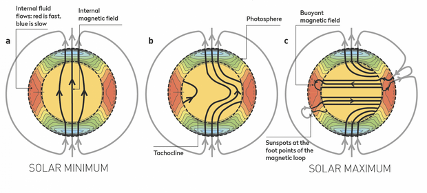
In this study, we consider two plausible TSI reconstructions from Connolly et al. (2023). Those from Hoyt and Schatten (1993) and from Bard et al. (2000), which Connolly et al. (2023) updated to the year 20182. The former TSI record (“H1993 Solar”) was based on the so-called multiproxy—i.e., equatorial solar rotation rate, sunspot structure, the decay rate of individual sunspots, the number of sunspots without umbrae, and the length and decay rate of the 11-yr sunspot activity cycle—reconstruction of the solar irradiance history.
1.2 Alternative hypotheses on temperature estimation
The IPCC’s attribution studies do not account for the direct effects of human activities on local temperatures (heat islands)—the second weakness addressed in this study. For example, heating and cooling of building interiors, electricity generation, manufacturing, freight and transport, asphalt and concrete, and where vegetation and open water have been removed or added. Where temperature readings are taken close to such human sources of heat or absence of natural cooling, they cannot properly reflect the individual effects of human emissions of carbon dioxide, etc., that the IPCC are concerned about (their Anthro variable), the Volcanic variable, and TSI.
To address this second limitation in the IPCC attribution studies, Connolly et al. (2021, 2023) developed four alternative estimates of surface temperatures that were intended to avoid heat island effects. They were based on rural only weather station readings, sea surface temperature readings, tree-ring width measurements, and glacier length measurements. For comparison with the approach used by the IPCC, they also developed an all-land temperature estimates series for the Northern Hemisphere.
 1.5 Hypotheses tested
The foregoing discussion suggests the following hypotheses, which are tested in this study.
-
- H1. Forecasts from causal models will [will not] be usefully more accurate than forecasts from a naïve no-change model.
- H2. Models using variable measures developed independently of the IPCC dangerous manmade global warming hypothesis will [will not] have greater predictive validity.
- H3. The statistical fit of the models (adjusted-R2) will not [will] be substantively positively related to their predictive validity.
- H4. Models using variable measures developed independently of the IPCC dangerous manmade global warming hypothesis will [will not] be more reliable.
Findings
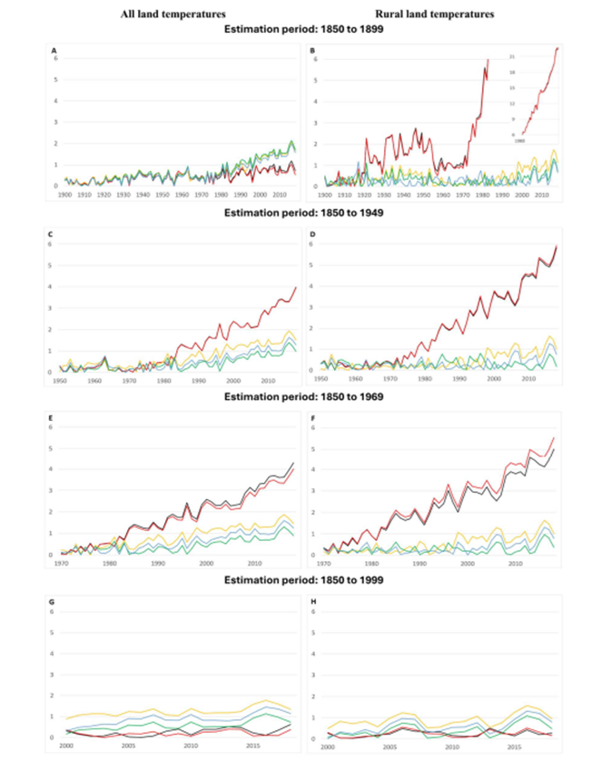
Figure 1: Absolute Errors of NH All Land and Rural Land Temperature Forecasts to 2018 (℃) — Forecasts from four alternative models plus naïve estimates over four periods. Legend (Causal variables in models): Black Anthro, Volcanic; Red Anthro, Volcanic, IPCC Solar; Green B2000 Solar, Volcanic; Blue H1993 Solar, Volcanic; Yellow Estimation sample median temperature.
3.1 Predictive validity of causal models versus naïve model [H1]
Forecast errors were larger than the benchmark errors (UMBRAE) for the IPCC Anthro models AVL and AVSL estimated with data from 1850 to 1949 and from 1850 to 1969, and for the AVR and AVSR models estimated with data from 1850 to 1899, 1850 to 1949, and 1850 to 1969. The anthropogenic warming models showed predictive validity relative the naïve model (UMBRAE less than 1.0) for only three of the eight combinations of forecast variable and estimation sample period.
3.2 Predictive validity of independent versus IPCC models [H2]
The MdAEs (median absolute error) of the forecasts from the models with IPCC’s anthropogenic and volcanic series as causal variables (AVL and AVR) and from the models that also included IPCC’s solar series (AVSL and AVSR) were greater than 1°C (roughly 2°F) for five of the eight combinations tested. The MdAEs of the forecasts from the models with B2000 solar and the volcanic series as causal variables (SBVL and SBVR) were less than 0.55°C (1°F) for all eight of the estimation periods used and temperature series being forecast combinations and for seven of the eight in the case of the models with H1993 as the solar variable (SHVL and SHVR).
3.3 Relationship between predictive validity and statistical fit of models [H3]
The correlations (sign-reversed Pearson’s r) between the accuracy of out-of-sample forecasts, as measured by UMBRAE (an error measure, hence the sign reversal), and the statistical fit of the models to the estimation data (adjusted-R2) for the causal models tested were large and negative for six (6) of the eight (8) combinations of estimation period (1850 to 1899, 1949, 1969, and 1999) used—and hence maximum forecast horizon of 119, 69, 49, and 19 years, respectively—and temperature series (NH Land and NH Rural) forecast.
3.4 Reliability of independent versus IPCC models [H4]
Charts of the results of Test 2 are presented in Figure 2 and are discussed below.
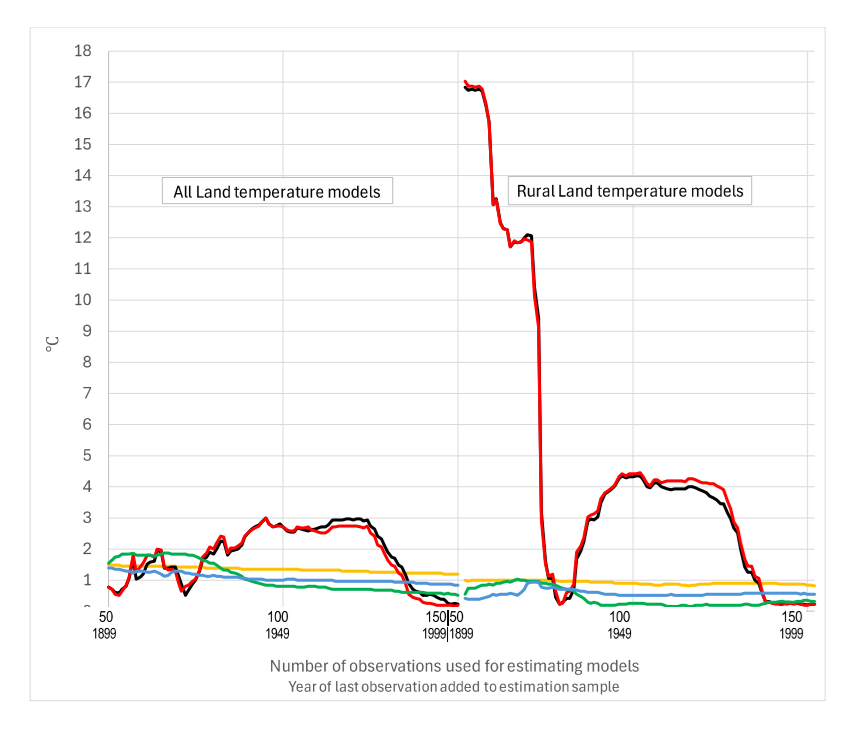
Figure 2. Median absolute errors of NH temperature forecasts 2000 to 2018 in ℃. Legend (Causal variables in models): Black Anthro, Volcanic; Red Anthro, Volcanic, IPCC Solar; Green B2000 Solar, Volcanic; Blue H1993 Solar, Volcanic; Yellow Estimation sample median temperature.
The independent solar models—SBVL and SHVL, and SBVR and SHVR—perform largely as one
would expect of causal models when forecasting using known values of the causal variables.
In the case of the AVR and AVSR models—forecasting the rural land temperatures, on the right of Figure 2—the MdAEs decreased rapidly from roughly 17 times the corresponding naïve forecast errors to beat the naïve MdAE when the 76th observation (1925) was added to the estimation samples. After that observation was added, the MdAEs for the AVR and AVSR model forecasts increased rapidly with each extra observation then stayed high before rapidly declining again after the 116th observation (1965) was added to the estimation samples.
When a model of causal relationships is estimated from empirical data on valid causal variables reliably measured, one would expect forecast errors to get smaller as more observations are used in the estimation of the model’s parameters. That is what the charts in Figure 2 show in the case of the naïve benchmark model forecasts and, broadly, what can be seen in the case of the independent models SBVL, SHVL, SBVR, and SHVR, but is not seen in the case of the models using the IPCC variables: AVL, AVSL, AVR, and AVSR.
The errors of the Anthro models’ forecast errors explode well beyond 1 °C and the benchmark model errors for forecast years beyond the mid-1970s, with puzzling exceptions. Namely, forecasts from Anthro models estimated from the largest sample size in the chart—1850 to 1999—and from models estimated from the smallest sample—1850 to 1899—forecasting All Land temperatures. In those cases, involving three of the eight charts, the Anthro model errors are less than the median historical temperature benchmark model errors, and mostly less than the errors of the independent models in later years.
The explosion in Anthro model errors from the 1970s is more extreme for models estimated to forecast Rural Land temperatures. Moreover, for the models estimated using only 1850 to 1899 data, errors are larger than those of the benchmark and independent models from 1920 and, prior to 1970, without any obvious pattern.
5. Conclusions
The IPCC’s models of anthropogenic climate change lack predictive validity. The IPCC models’ forecast errors were greater for most estimation samples —often many times greater—than those from a benchmark model that simply predicts that future years’ temperatures will be the same as the historical median. The size of the forecast errors and unreliability of the models’ forecasts in response to additional observations in the estimation sample implies that the anthropogenic models fail to realistically capture and represent the causes of Earth’s surface temperature changes. In practice, the IPCC models’ relative forecast errors would be still greater due to the uncertainty in forecasting the models’ causal variables, particularly Volcanic and IPCC Solar.
The independent solar models of climate change—which did not include a variable representing the IPCC postulated anthropogenic influence—do have predictive validity. The models reduced errors of forecasts for the years 2000 to 2018 relative to the benchmark errors for all, and all but one of 101 estimation samples tested for each of the two models. One of the models (B2000 Solar) reduced errors by more than 75 percent for forecasts from models estimated from 35 of the samples—a particularly impressive improvement given that the benchmark errors were no greater than 1 °C for all but one of the estimation samples.
The independent solar models provide realistic representations of the causal relationships with surface temperatures. The question of whether the independent solar variables can be forecast with sufficient accuracy to improve on the benchmark model forecasts in practice, however, remains relevant. All in all, and contra to the IPCC reports, there is insufficient evidential basis for the use of carbon dioxide, et cetera, emissions—taken together, the IPCC’s Anthro—as climate policy variables.
Finally, this study provides further evidence that measures of statistical fit provide misinformation about predictive validity. Predictive validity can only be properly estimated when the proposed model or hypothesis is used for forecasting new-to-the-model data, and the forecasts are then compared for accuracy against forecasts from a plausible benchmark model. This important conclusion needs bearing in mind when evaluating policy models.
See Also:
Lacking Data, Climate Models Rely on Guesses

Figure 1. Anthropgenic and natural contributions. (a) Locked scaling factors,
weak Pre Industrial Climate Anomalies (PCA). (b) Free scaling, strong PCA
Climate Models Hide the Paleo Incline


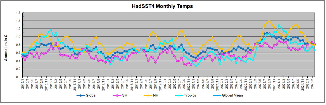
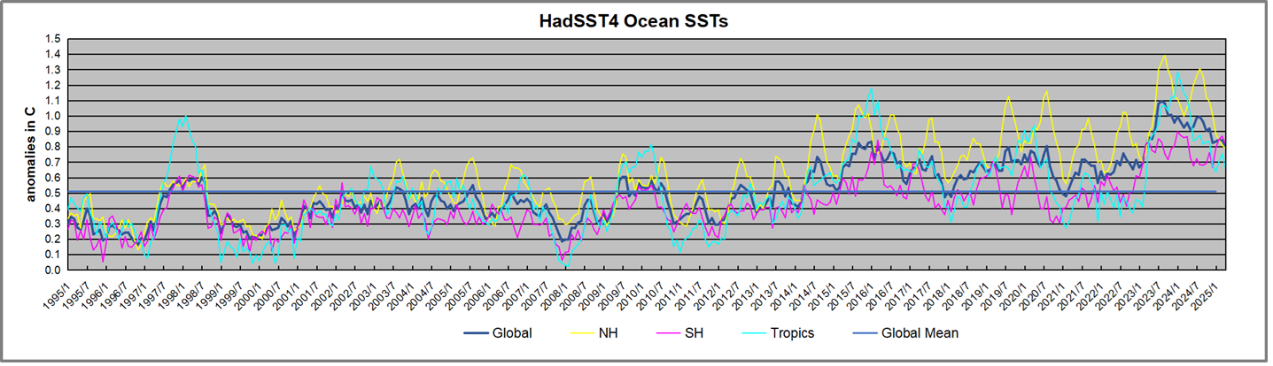
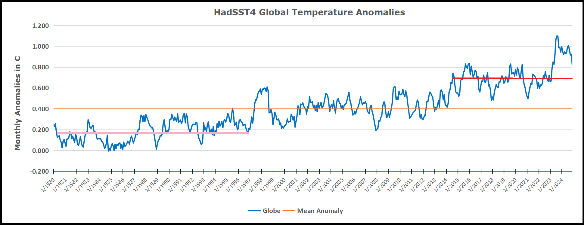
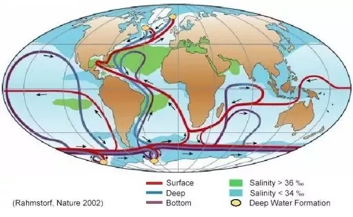
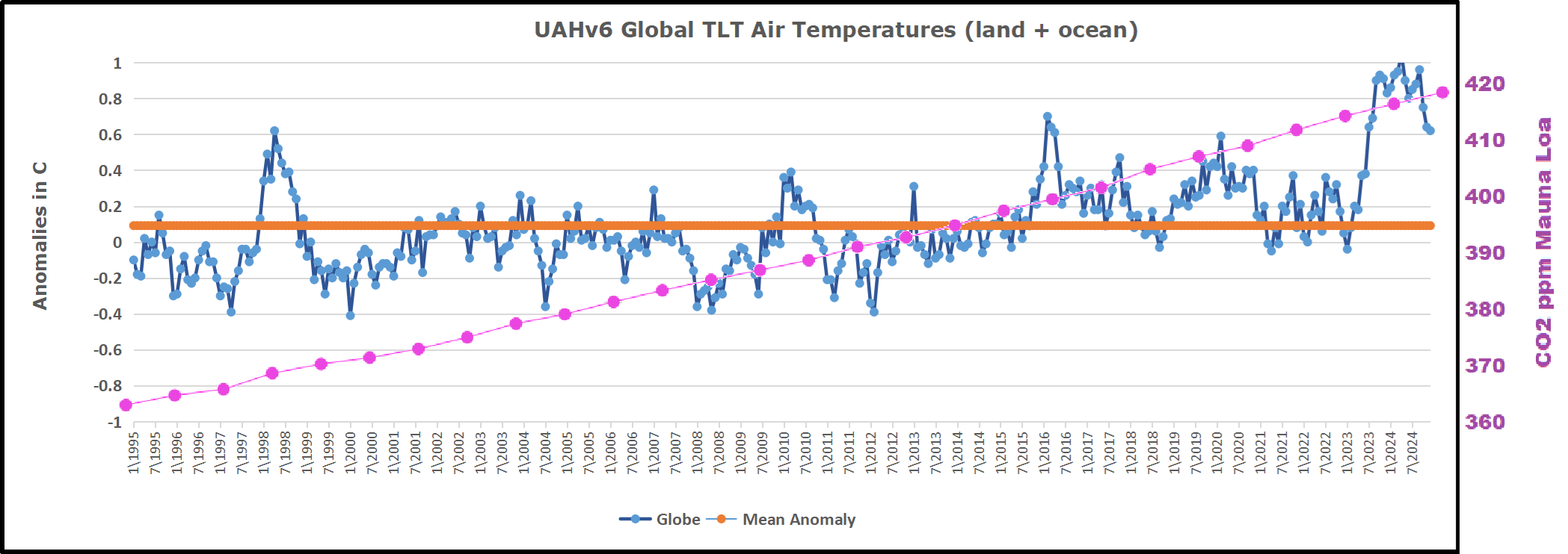
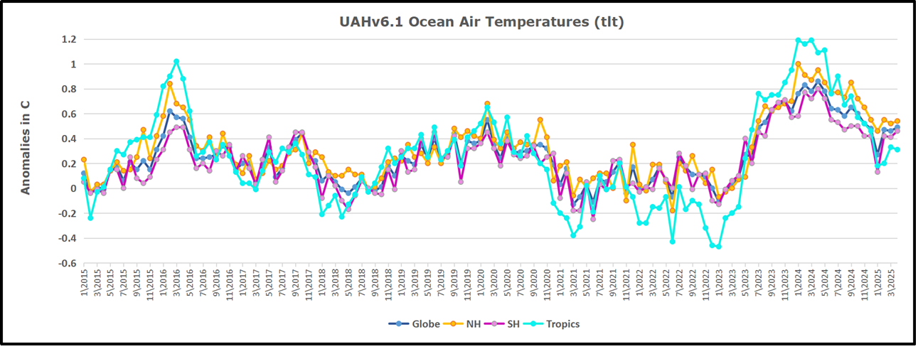
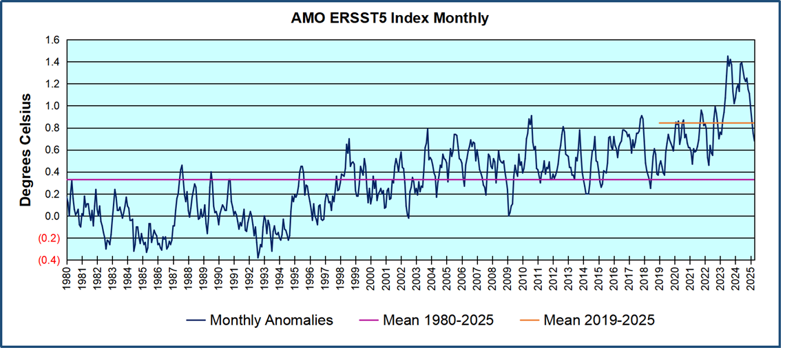
 The best context for understanding decadal temperature changes comes from the world’s sea surface temperatures (SST), for several reasons: