This is an update correcting a previous post Fear Not CO2! I discovered math errors that invalidated the main conclusion. I apologize for not seeing the problem before posting.
NO it is not even an issue you need to worry about.
Look closely. The biological adaptation is eating up the CO2 almost as fast as it is being emitted and the adaptation is getting faster every year.
Out of the over 38 GT output in 2019 only 0.02 GT will not be sequestered naturally and by next year that will be gone. The plants are eating up the CO2 just a few days after the release. They are happily eating it up just fine. You don’t even need to plant trees. Nothing against trees here. I like them.
This is the TRUMP CARD on the game. With this known, it is impossible to imagine the problems proposed are happening regardless of all other issues.
Correction Update
I reblogged an answer from Quora with an analysis and conclusions new to me. I thought it interesting if it held up to scrutiny.. Afterward I became uncomfortable when double checking the math, and so I am retracting my support. One smaller issue was noted in my post regarding CO2 having a larger weight (44) than the average air molecule (29). Thus calculating CO2 mass in the atmosphere should apply a ratio of 1.52. That does not in itself materially affect the finding.
The Table produced by Paul Noel is shown above..
The more substantial issue is having equivalent units of mass for comparing atmospheric CO2 and human emissions of CO2. The proper unit is Gigatons since that is how emissions are reported. One GT is defined as 1 billion (10^9) metric tons and 1 metric ton is 1000 (10^3) kilograms. So one GT is 10^12 kg.
The mass of the atmosphere is calculated using air pressure and area, with a little variation in the results obtained by researchers. A typical standard is 5.148 x 10^18 kg. That converts to 5148000 x 10^12 kg or 5148000 GT. Once that value is plugged into the table, the results are very different. I had recognized that 10^15 was not GT, but thought it was only mislabeling. Later I found that the comparison was distorted in the process.
My revised Table 1 applies a weighted calculation for CO2 compared to average air molecules and derives masses and percentages using GT consistently.
It is clear that the claim of 99% sequestration of emissions is an artifact of faulty math. A better approximation is 57% for emissions reduced by natural fluxes.
This does not mean we should fear CO2. For one thing the greening of the planet and record annual crop yields are a great benefit from both warming and higher atmospheric CO2. It is also the case that estimates of human emissions (fraught with uncertainty) are small compared to natural fluxes, which are estimated with error ranges exceeding emission amounts. Further, the sensitivity of temperature to rising CO2 is assumed to lie in a wide range.
Roy Clark explains how climate science built an house of cards obscuring the actual physical mechanisms driving observed climate fluctuations. Text of his recent post at WUWT in italics with my bolds.
The basic issue is that there is no such thing as a climate sensitivity to CO2 or any other so called ‘greenhouse gas’. Radiative forcing can politely be described as climate theology – how does a change in the atmospheric concentration of CO2 change the number of angels that may dance on the head of a climate pin? The climate equilibrium assumption was used by Arrhenius in his 1896 estimate of global warming. In this paper he traced the concept back to Pouillet in 1838. Speculation that changes in atmospheric CO2 concentration could somehow cause an Ice Age started with John Tyndall in 1863.
To get to the bottom of the radiative forcing nonsense it is necessary to go back to Fourier in 1827 and start over with the real physics of the surface energy transfer.
The essential part that almost everyone seems to have missed in this paper is the time delay or phase shift between the solar flux and the surface temperature response. The daily phase shift in MSAT can reach 2 hours and the seasonal phase shift can reach 6 to 8 weeks. This is clear evidence for non-equilibrium thermal storage. The same kind of non-equilibrium phase shift on different time and energy scales occurs with electrical energy storage in capacitors and inductors in AC circuits – low pass filters, tank circuits etc.
The equilibrium average climate assumption was used by Manabe and Wetherald (M&W) in their 1967 climate modeling paper. They abandoned physical reality and created global warming as a mathematical artifact of their input modeling assumptions. The rest of the climate modelers followed like lemmings jumping off a cliff. In the 1979 Charney report, no-one looked at the underlying assumptions. The radiative transfer results were reasonable –for the total long wave IR (LWIR) flux at the top and bottom atmosphere – and the mathematical derivation of the flux balance equations was correct. The increase in surface temperature was the a-priori expected result. Radiative forcing and the invalid equilibrium flux balance equations were discussed by Ramanathan and Coakley in 1978. The prescribed mathematical ritual of radiative forcing in climate models was described by Hansen et al in 1981. They also introduced a fraudulent ‘slab’ ocean model and did a bait and switch from surface to weather station temperatures.
The LWIR flux interacts with the surface, not the weather station thermometer at eye level above the ground.
Radiative forcing is still an integral part of IPCC climate models [IPCC, 2013]. Physical reality has been abandoned in favor of mathematical simplicity. Among other things, M&W threw out the Second Law of Thermodynamics along with at least 4 other Laws of Physics. The underlying requirement for climate stability is that the absorbed solar heat be dissipated by the surface. This requires a time dependent thermal and or humidity gradient at the surface.
The starting point for any realistic climate system is that the upward LWIR flux from the top of the atmosphere does not define an equilibrium average temperature of 255 K. Instead it is the cumulative cooling flux emitted from multiple levels down through the atmosphere. The upward emission from each level is then attenuated by the LWIR absorption/emission along the upward path to space [Feldman et al, 2008]. Another fundamental error in the radiative forcing argument is the failure to consider the molecular line width effects. Part of this was due to the band model simplifications that are still used in the climate models to speed up the calculations. The IR flux through the atmosphere consists of absorption and emission from many thousands of overlapping molecular lines, mainly from CO2 and water vapor [Rothman et al, 2005].
As the temperature and pressure decrease with altitude, these lines become narrower and transmission ‘gaps’ open up between the lines. This produces a gradual transition from absorption/emission to a free photon flux to space.
The radiative forcing argument has also obscured the fact that the heat lost to space is replaced by convection, not LWIR radiation. The troposphere is an open cycle heat engine that transports heat from the surface by moist convection. It is stored in the troposphere as gravitational potential energy. As a high altitude air parcel cools by LWIR emission, it contracts and sinks back down through the troposphere. The upward LWIR flux to space is decoupled from the surface by the linewidth effects. The downward LWR flux from the upper troposphere cannot reach the surface and cause any kind of change in the surface temperature. Almost all of the downward LWIR flux reaching the surface originated from within the first 2 km layer of the troposphere and about half of this comes from the first 100 m layer.
Figure 2: Thermal reservoirs, surface energy transfer and thermal storage (schematic). The surface is heated by the sun and cooled by a combination of net LWIR emission, convection and evaporation. Heat is stored below the surface and released over a range of time scales. There is no ‘equilibrium average temperature’. Source: Roy Clark
Near the surface, the lines in the main bands for CO2 and water vapor are sufficiently broadened that they merge into a continuum. There is an atmospheric transmission window in the 8 to 12 micron spectral region that allows part of the surface LWIR flux to escape directly to space. The magnitude of this transmitted cooling flux varies with cloud cover and humidity. The downward LWIR flux to the surface from the broad molecular emission bands provides an LWIR exchange energy that ‘blocks’ the upward LWIR flux from the surface. Photons are exchanged without any net heat transfer.
In order for the surface to cool, it must heat up until the excess absorbed solar heat is removed by moist convection. This is the real cause of the so called ‘greenhouse effect’.
It requires the application of the Second Law of Thermodynamics to the surface exchange energy. There is no equilibrium average climate so there can be no average ‘greenhouse effect temperature’ of 33 K. Instead, the greenhouse effect is just the downward LWIR flux from the lower troposphere to the surface. It can be defined as the downward flux or as an ‘opacity factor’ [Rorsch, 2019]. This is the ratio of the downward flux to the total blackbody surface emission.
The surface temperature has to be calculated at the surface using the surface flux balance. The change in local surface temperature is determined by the change in heat content or enthalpy of the local surface thermal reservoir divided by the specific heat [Clark, 2013a, b]. The LWIR flux cannot be separated from the other flux terms and analyzed independently. The land and ocean surface behave differently and have to be considered separately.
Over land, the various flux terms interact with a thin surface layer. During the day, the surface heating produces a thermal gradient both with the cooler air layer above and the subsurface layers below. The surface-air gradient drives the convection or sensible heat flux. The subsurface thermal gradient conducts heat into the first 0.5 to 2 meter layer of the ground. Later in the day this thermal gradient reverses and the stored heat is released back into the troposphere. The thermal gradients are reduced by evaporation if the land surface is moist. An important consideration in setting the land surface temperature is the night time convection transition temperature at which the surface and surface air temperatures equalize. Convection then essentially stops and the surface continues to cool more slowly by net LWIR emission. This convection transition temperature is reset each day by the local weather conditions.
The ocean surface is almost transparent to the solar flux. Approximately 90% of the solar flux is absorbed within the first 10 m ocean layer. The surface-air temperature gradient is quite small, usually less than 2 K. The excess absorbed solar heat is removed through a combination of net LWIR emission and wind driven evaporation. The penetration depth of the LWIR flux into the ocean surface is 100 µm or less and the evaporation involves the removal of water molecules from a thin surface layer [Hale and Querry, 1972]. These two processes combine to produce cooler water at the surface that sinks and is replaced by warmer water from below. This is a Rayleigh-Benard convection process, not simple diffusion. There are distinct columns of water moving in opposite directions. The upwelling warmer water allows the wind driven ocean evaporation to continue at night. As the cooler water sinks, it carries with it the surface momentum or linear motion produced by the wind coupling at the surface. This establishes the subsurface ocean gyre currents. Outside of the tropics there is a seasonal phase shift that may reach 6 to 8 weeks.
This phase shift can only occur with ocean solar heating. The heat capacity of the land thermal reservoir is too small to produce this effect. In many parts of the world, the prevailing weather systems are formed over the ocean. The temperature changes related to the ocean surface are stored by the weather system as the bulk surface air temperature and this information can be transported over very long distances. Such ocean related phase shifts can be found in the daily climate data for weather stations in places like Sioux Falls SD.
Over the oceans, the wind driven evaporation can never exactly balance the solar heating. This produces the ocean oscillations such as the ENSO, PDO and AMO.
These surface temperature changes are incorporated into the various weather systems and can be seen in the long term climate data, particularly the minimum MSAT. The whole global warming scam is based on nothing more than the last AMO warming cycle coupled into the weather station data [Akasofu, 2010].
Figure 1: Change in wind speed (cm s-1) needed to restore the ocean surface cooling flux when the downward LWIR flux is increased by 2 W m-2 Both the fixed and the temperature dependent LWIR window flux cases are shown.
A fundamental failure of the radiative forcing argument is the lack of any error analysis. Over the last 200 years, the atmospheric CO2 concentration has increased by a little over 120 ppm. This has produced an increase in the downward LWIR flux at the surface of about 2 W m-2 [Harde, 2017]. Over the oceans this is coupled into the first 100 micron layer of the ocean surface. Here it is fully coupled to the wind driven evaporation. Using long term ocean evaporation data from Yu et al, 2008, an approximate estimate of the evaporation rate within the ±30 degree latitude region is 15 Watts per square meter for each change in wind speed of 1 meter per second.
This means that the radiative forcing from an increase of 120 ppm in the CO2 concentration amounts to a change in wind speed of about 13 CENTIMETERS per second.
This is at least two orders of magnitude below the normal variation in ocean wind speed. Similarly, a reasonable estimate of the bulk convection coefficient for dry land is 20 Watts per square meter per degree C difference between surface and air temperature. Here a 2 W m-2 change in convection requires a change of 0.1 C in the surface air thermal gradient.
Once the physics of the time dependent surface energy transfer is restored, global warming and radiative forcing disappear into the realm of computerized climate fiction.
The topic of radiative forcing was recently reviewed in detail by Ramaswamy et al [2019] as part of the American Meteorological Society monographs series. This review provides a good start for a scientific and criminal fraud investigation into the climate modeling fraud. To begin, the scientific community should demand that this particular monograph be retracted and all further work on equilibrium climate modeling be stopped. Any climate model that uses radiative forcing is by definition invalid. There is no need to try and validate the computer code of any equilibrium climate model. The use of radiative forcing alone is sufficient to render the results totally useless. These modelers are not scientists, they are mathematicians playing with a set of physically meaningless equations. They left physical reality behind when they made the climate equilibrium assumption. They are now members of a rather unpleasant quasi-religious cult. They believe that the divine spaghetti plots created by the computer climate models come from a higher authority that the Laws of Physics.
Figure 12: The ocean surface energy balance in the tropical warm pool. The evaporative surface cooling is strongly dependent on the wind speed. Source: Roy Clark
Any realistic climate model must correctly predict the changes in ocean temperature caused by the ocean oscillations. These must then be used to predict the changes in the weather station data.
This must include the minimum and maximum surface air temperatures, surface temperatures and the phase shifts. There are no forcings, feedbacks or climate sensitivities, just time dependent rates of heating and cooling. It is time to welcome the Second Law of Thermodynamics back to the climate models. It has always been part of the Earth’s climate system. [See linked post for references]
Roy Clark’s research studies are available at his website Ventura Photonics
[I just noticed that Quora buried Walker’s 12 point answer to the query, and only shows others’ comments afterward. In order to see the actual response you have to go here: https://www.quora.com/profile/John-Walker-922/answers
and then search for “skeptics”. There are many persuasive exhibits there, perhaps the reason for suppressing the document.]
An extensive and documented reply is given at Quora from John Walker, former Laboratory Medical Director/Pathologist (1984-2011). Excerpts in italics with my bolds.(red text is link).
There are very few individuals who are skeptical that the climate changes. But there are millions and millions of individuals (and growing), who are quite skeptical that human emissions of CO2 are causing apocalyptic global warming, including many scientists, climate scientists, Nobel Laureates, and other highly educated individuals.
The reason for this is multi-factorial and very voluminous. The following presents condensed summaries of 12 of the reasons that so many individuals have become highly skeptical of the theory of CAGW. Even though it is rather long, it represents only a small portion of the information, studies and references engendering skepticism of this unproven assemblage of hypotheses. Most of it is taken from my 250+ page treatise on the fallacies of the theory of CAGW.
1 . First and foremost is the fact that there is currently NO experimental evidence validating the theory of CAGW. Rather CAGW is a collection of unproven/unvalidated hypotheses, which can only be accepted by faith. However, most of these hypotheses have been shown to contain fallacies and/or misinformation.
2 . The “science” behind the theory of CAGW has not been sufficiently rigorous, non-biased, or open, and, crucially, does not comply with the tenets of the scientific method since it is not subject to potential falsification by testing/experiment.
3 . The theory of CAGW is based entirely upon:
a . Atmospheric CO2 versus temperature correlation studies(which are not proof of cause and effect, are partially based upon fictitious/manipulated/estimated temperature data [as in the “hockey stick” graph and altered NASA/NOAA/CRU data], and actually do not correlate all that well):
The original MBH graph compared to a corrected version produced by MacIntyre and McKitrick after undoing Mann’s errors.
b . Partially altered, manipulated, selective, imprecise, incomplete, extrapolated and unverified/fictitious temperature data (as revealed by Climategate, the “Hockey Stick” confutation, and other sources), with frequent measurements selected from urban concrete and asphalt hot spots, naturally producing higher temps, which increase in number over time due to continued urban growth).
“Government reports, writers of opinion pieces, and bloggers posting graphs purporting to show rising or record air temperatures or ocean heat, are misleading you. This is not actual raw data. It is plots of data that have been ‘adjusted’ or ‘homogenized’ (i.e., manipulated) by scientists – or it is output from models that are based on assumptions, many of them incorrect. UK Meteorological Office researcher Chris Folland makes no apologies for this. ‘The data don’t matter. We’re not basing our recommendations [for reductions in carbon dioxide emissions] upon the data. We’re basing them upon the climate models’.” Climate: The Real ‘Worrisome Trend’ (Part I: Faulty Science) – Master Resource
c . Unreliable computer models(based upon partially altered, manipulated, selective, imprecise, incomplete, extrapolated and unverified/fictitious temperature data, woefully inadequate/incomplete input data regarding thousands of climate parameters, and “educated guesses” about the climate sensitivity to atmospheric CO2), which can be programmed to reveal whatever result the programmer desires, and many of which have already been proven incorrect or exaggerated.
d . Insufficient understanding of the role and relative magnitude/sensitivity of CO2 as a “greenhouse” gas,and the unproven (and many would say ludicrous) hypothesis thatthe earth’s atmosphere (with all its enormity, complexity, multiple layers, convection, layers of exceedingly cold air [as low as -60F] and even colder adjacent outer space [-455F] as well as extremely hot (high kinetic energy) upper layers, huge underlying oceans with complex currents and temperature fluctuations, varying molecular compositions, stratospheric ozone [which absorbs both UV and IR radiation], variable humidity, massive heat-absorbing evaporative processes, extensive cloud formations, variably intense winds, the jet stream, varying barometric pressures, cosmic ray effects, and NO glass ceiling or walls) functions identically to a glass-enclosed greenhouse. (Yes, that does seem rather ludicrous!)
5 . Promoters of the theory of CAGW falsely claim there is a 97% “consensus” among climate scientiststhat the theory is true. Indeed the 97% figure is false and based upon poorly contrived surveys/studies by CAGW promoters and “peer-reviewed” (i.e., “pal-reviewed”) by other CAGW promoters. If one reads the original papers where the 97% figure was contrived, it is quite easy to see how poorly designed and biased these surveys were. All of these surveys/studies have been debunked by multiple statistical analyses and better defined and controlled surveys and studies, revealing that less than half of climate scientists believe in the theory of CAGW.
“Claims that a ‘consensus’ exists among climate experts regarding the causes of the modest warming of the past century are contradicted by thousands of independent scientists.” – International Climate Science Coalition Core Principles
The fact is that tens of thousands of scientists, including climate scientists and many Nobel Laureates, do NOT accept the theory of CAGW:[Numerous examples are provided in linked article]
6 . Thus, in essence, CAGW promoters are demanding we accept their conclusions based upon consensus and faith(normally antithetical to most modern liberals’ thinking), just as theocrats and other religious fundamentalists argue. But the inability to follow the rigorous scientific method by the use of repeatable double blind, controlled experiments for validation does not justify acceptance of a theory without such experiments simply because they cannot be performed. It may be fine to accept beliefs by consensus or even by faith on personal or other matters which do not materially affect other people. But those pushing the theory of CAGW are demanding draconian changes affecting everyone on the planet, such as diverting tens of trillions of dollars from solving known existing existential problems (poverty, hunger, violence, war, infectious disease, cancer research, pollution and over-fishing of our oceans, lack of adequate sanitation, education and clean water, etc.) in order to “fight” an unproven future potentially existential problem with costly methods which have not been proven effective, replacing capitalism and democracy with global socialism and authoritarian one world government, and redistributing global wealth. Such actions would be premature, irresponsible, illogical, socialistic, cruel and lead to massive morbidity and mortality!
7 . In addition to the “97% consensus” falsehood, CAGW promoters and alarmists have promulgated many other lies, failed predictions (for both catastrophic global cooling and global warming) based upon their flawed computer models, abundant misinformation and disinformation. If the theory of CAGW is true, why the need to prevaricate? Anyone who is aware of this widespread sophistry must become skeptical of the theory. [Many examples are given in the linked article]
8 . Another clue that the theory of CAGW is fallacious is the fact that many promoters and alarmists so frequently resort to ad hominen attacks or demand that skeptics be banned from discussions.The former is another logical fallacy, which is used when the promoter has no real evidence to back up his/her claim and is unable to respond in a logical and respectful manner. They feel cornered because of their lack of intelligent retort. They hope that such attacks will make the skeptic afraid to make further comments.
Banning and refusing to hear/discuss information contrary to one’s dogmatic belief is characteristic of a fundamentalist who has been indoctrinated, often with propaganda. It is characteristic of religious fanaticism, not science. While it is prohibited under Quora policy, you will discover that some CAGW alarmist authors just can’t stop themselves from indulging in this fallacious and destructive tactic.
Again, this engenders more skepticism in their beliefs.
9 . Climategate.Climategate was a notorious event initiated by leaked emails in 2009 (with a second batch released in 2011) allegedly revealing the deceit and deception practiced by a prominent group of British (Climatic Research Unit or CRU) and American climate researchers (including Michael Mann of Penn State) who promote the theory of CAGW and supply much of the climate and temperature data and reports to the IPCC. The latter gives this group tremendous influence regarding the UN’s climate change agenda.
“There are three threads in particular in the leaked documents which have sent a shock wave through informed observers across the world. Perhaps the most obvious, as lucidly put together by Willis Eschenbach (see McIntyre’s blog Climate Audit and Anthony Watt’s blog Watts Up With That ), is the highly disturbing series of emails which show how Dr Jones and his colleagues have for years been discussing the devious tactics whereby they could avoid releasing their data to outsiders under freedom of information laws.
“But the question which inevitably arises from this systematic refusal to release their data is – what is it that these scientists seem so anxious to hide? The second and most shocking revelation of the leaked documents is how they show the scientists trying to manipulate data through their tortuous computer programmes, always to point in only the one desired direction – to lower past temperatures and to ‘adjust’ recent temperatures upwards, in order to convey the impression of an accelerated warming. This is what Mr McIntyre caught Dr Hansen doing with his GISS temperature record last year (after which Hansen was forced to revise his record), and two further shocking examples have now come to light from Australia and New Zealand.
“The third shocking revelation of these documents is the ruthless way in which these academics have been determined to silence any expert questioning of the findings they have arrived at by such dubious methods – not just by refusing to disclose their basic data but by discrediting and freezing out any scientific journal which dares to publish their critics’ work. It seems they are prepared to stop at nothing to stifle scientific debate in this way, not least by ensuring that no dissenting research should find its way into the pages of IPCC reports.”
10 . The IPCC, which is the primary authority driving the CAGW agenda is a political body, not a scientific body. It’s originating mission was to find human causes of climate change.
“It is to specifically find and report a human impact on climate, and thereby make a scientific case for the adoption of national and international policies that would supposedly reduce that impact.
[Thus, the IPCC has been directed to attribute the cause, or at least significant portions of the cause, of climate change to human influences. If it does not make claims of significant human influence, it’s function would be obviated and its members likely out of their UN jobs!]
“The IPCC is also designed to put political leaders and bureaucrats rather than scientists in control of the research project. It is a membership organization composed of governments, not scientists. The governments that created the IPCC fund it, staff it, select the scientists who get to participate, and revise and rewrite the reports after the scientists have concluded their work. Obviously, this is not how a real scientific organization operates.
11 . Much of the motive behind the promotion of the theory of CAGW is driven by money, power, and politics.Socialists, globalists and radical environmentalists are using the fear of CAGW to convince the world to replace capitalism with authoritative global socialism. The climate change industry now exceeds $1.5 trillion. If “cap-and-trade” legislation is ever passed in the US, as Al Gore, Goldman-Sachs, and other wealthy investors hope, they could potentially make $trillions via the buying and selling of carbon credits on a commodities exchange. Gore and Goldman tried desperately to get such legislation passed during the Obama administration. They were major investors in the Chicago Climate Exchange, which would have been the commodities exchange for carbon credits.
12 . There are better alternative theories regarding the mechanisms that drive the earth’s climate.Most of the theories derive from the observation that the earth’s climate goes through multiple, well-defined cycles (and cycles within cycles) of warming and cooling, and have done so for millennia. They generally involve various changes in total solar radiation reaching the earth and the adiabatic heating of the earth’s atmosphere due to atmospheric pressure. The theory of Cosmoclimatology is gaining credence among many climate scientists and astrophysicists.
Many other theories about the cause of climate change also involve solar influences. Think of the extreme temperature changes that are caused by changes in the amount of solar radiation the earth receives. Just the variation in the tilting of the earth leads to 4 seasons with temperatures varying from over 100 F to minus 20 F (or even colder) between summer and winter months in many locations. Temperatures increase dramatically just by moving towards the equator from higher or lower latitudes, due to differences in solar radiation. Day and night temperatures can easily differ by as much as 30 F or more, all in a 12 hour span. Temperatures on a sunny summer day can drop by 5 F in a matter of seconds if a cloud passes overhead. Compare that to the claimed increase in global temp of 1.4 F over 150 years supposedly caused by anthropogenic CO2.
In addition to the multiple periodic clusterings creating grand solar minima and maxima, there are multiple additional cyclic changes of solar activity, which are being elucidated with continuing climate research (another reason to stop making the absurd, counter-productive and pseudoscientific claim that the “science is settled”). There are centennial and bicentennial cycles of grand solar minima and maxima, along with many other cyclic processes of longer time intervals related to celestial changes:
There have been numerous glacial cycles, each lasting an average of 100,000 years. They coincide with the Milankovitch Eccentricity cycle of the earth’s orbit around the sun. Within each cycle is a period of marked global cooling (lasting from 70k to 90k years in which immense glaciers cover much of the land surface, and much of the ocean surface freezes. The cold periods are followed by interglacial (warm) periods lasting from 10k to 30k years. Some climatologists believe that the Earth is on the downward slope of the current interglacial period and headed towards the next ice age, which could arrive in the next several thousand years. During this downward slope, global temperatures are expected to slowly decrease with intermittent warmer and cooler trends. Milankovitch cycles – Wikipedia
And there is so much more but not enough time and space to present it all.
Thanks to Andreas Müller for writing at his blog hintermbusch on four key presentations at the EIKE Climate Conference on Nov. 23, 2019. As many have read, eco-terrorists forced the sessions out of the scheduled venue, but the gatherings went on elsewhere. So much for dialogue in search of scientific truth. Here are some excerpts in italics with my bolds to encourage readers to read his informative report. (link in red above).
In this blog post, I summarize these lectures and add links to the video clips for you to follow the lectures on your own and in full detail (Only the first talk was in German and is not easily accessible for most of the international public).
Christian Schlüchter, Switzerland
Prof. em. Christian Schlüchter is a geologist and has studied the glaciers of the Alps in great detail. He reports the findings of very old timber in and below glaciers and what those trees taught him about the glacial epochs of the Alps.
One of the most intuitive finds of Schlüchter’s is this huge tree trunk, found at a glacier tongue (see the most beautiful glacier snout behind!).
This place nowadays is clearly above the limit of vegetation and still there is this tree which attracted Schlüchter’s curiosity and fuelled his research: How old is it? Where and under what conditions has it grown and why is it here.
The key message from his slides is that all of these records were left in times when the alpine glacier extent was smaller than in 2005.
Warm periods: more life
The timberline was at least 300 meters higher which indicates a minimum of 1.8° C higher temperatures. An example of this gives Hannibal, who managed to cross the Alps with elephants because the higher regions were much less covered by ice than in recent centuries.
Warm periods: more civilization
As his summary, Schlüchter gave the following facts:
More than 50% of the last 11000 years alpine glaciers were smaller than 2005
This fact he baptized, “dominance of the Hannibalistic world”
Alpine glaciers have shown huge dynamics
Events of glacier growth were fast and short
The little ice age (from the end of the medieval warm period to about 1850) was the longest glacier extension since the last ice age 12000 years ago
Every warming followed an accelerated glacier growth
Nicola Scafetta, Italy
Nicola Scafetta is an italian physicist und climate modeller who works at Naples university. He is well-known for his criticism of IPCC climate models and, of course not uncontested for creating his own climate models and comparing them to IPCC results. His talk in Munich again took aim at the weaknesses und faults of IPCC climate models.
He notes that the models tend to reproduce the notorious “hockeystick” shape and therefore fail at the medial warming bump! (This is an echo of a very old climate change controversy, documented here).
He also shows similar failures for longer periods and demonstrates that the ulimate reason for this is that the models are not capable of reproducing climate variations which follow periodic solar activity.
Therefore, ten years ago, he contrasted his own model forecasts, which take those into account, (black line) to those of the IPCC (dashed blue line), which leads to the climax of the talk Below is an upadated graph of his 2010 projections (cyan color) compared to observations and to IPCC models (green).
Nir Shaviv, Israel
Nir Shaviv is a well-known but moderate climate skeptic. Besides the lecture on alpine glaciers by Christian Schlüchter, he was my main reason to choose this half day from the conference program. Shaviv continued where Scafetta had ended and discussed the IPCC world and its errors.
For a start, he presented its lines of thinking:
Next, he discussed the validity of each building block, marked the errors und deconstructed the standard picture. He emphasized that the climate sensitivity of CO2 is a priori unknown and largely overestimated by the IPCC. He judged it a severe shortcoming that other forcings than green house gases are ruled out by the IPCC: the sun!
He pointed out that the IPCC overestimates climate sensitivity of CO2 at the expense of solar influences. While IPCC modelers managed to hide this for 20th century data, it will lead to a serious overestimate of temperatures in the 21st when solar influences will be cooling. He therefore expects a much lower temperature rise than predicted by the IPCC, a modest (and manageable) one:
Using physical arguments Shaviv manages to set an upper limit for the climate sensitivity of CO2. This should convince the audience to accept additional forcings behind the 20th century temperature rise. Like Scafetta he points at a solar driven forcing.
Henrik Svensmark, Denmark
Henrik Svensmark is a Danish physicist und climate researcher. As other speakers he reports that he finds it more and more difficult to raise funds for his research because its results contradict the IPCC position:
By experiments and also by correlation measurements Svensmark has investigated this mechanism of cloud creation by cosmic rays. This is interesting because IPCC researchers cite reduction of cloud creation by global warming as a possible positive feedback mechanism which could escalate global warming to catastrophic levels. Svensmark assumes that it provides a way how solar activity, via its solar winds, has a climate impact on the earth which adds to the direct impact of solar irradiation to the earth.
Scientific summary
As a physicist I found all 4 talks interesting. They demonstrate that real and sophisticated science on climate was presented at that conference. Nothing suggests that this is less serious or valid science than anything I experienced during my time as a master and Ph.D student in physics. The presented results make it seem rather improbable that the climate models of the IPCC are complete, beyond any doubt or worth a 97% consensus.
H/T to Ice Age Now for pointing to this brief and informative video of Bill Sellers explaining our planet’s climate cycles due to astronomical factors described by Milankovitch.
I just hope during her time-out Greta takes a look and learns something from this video.
Methane alarm is one of the moles continually popping up in the media Climate Whack-A-Mole game. An antidote to methane madness is now available to those inquiring minds who want to know reality without the hype.
Methane and Climate is a paper by W. A. van Wijngaarden (Department of Physics and Astronomy, York University, Canada) and W. Happer (Department of Physics, Princeton University, USA) published at CO2 Coalition November 22, 2019. It is a summary in advance of a more detailed publication to come. Excerpts in italics with my bolds.
Overview
Atmospheric methane (CH4) contributes to the radiative forcing of Earth’s atmosphere. Radiative forcing is the difference in the net upward thermal radiation from the Earth through a transparent atmosphere and radiation through an otherwise identical atmosphere with greenhouse gases. Radiative forcing, normally specified in units of W m−2 , depends on latitude, longitude and altitude, but it is often quoted for a representative temperate latitude, and for the altitude of the tropopause, or for the top of the atmosphere.
For current concentrations of greenhouse gases, the radiative forcing at the tropopause, per added CH4 molecule, is about 30 times larger than the forcing per added carbon-dioxide (CO2) molecule. This is due to the heavy saturation of the absorption band of the abundant greenhouse gas, CO2. But the rate of increase of CO2 molecules, about 2.3 ppm/year (ppm = part per million by mole), is about 300 times largerthan the rate of increase of CH4 molecules, which has been around 0.0076 ppm/year since the year 2008.
So the contribution of methane to the annual increase in forcing is one tenth (30/300) that of carbon dioxide. The net forcing increase from CH4 and CO2 increases is about 0.05 W m−2 year−1 . Other things being equal, this will cause a temperature increase of about 0.012 C year−1 . Proposals to place harsh restrictions on methane emissions because of warming fears are not justified by facts.
The paper is focused on the greenhouse effects of atmospheric methane, since there have recently been proposals to put harsh restrictions on any human activities that release methane. The basic radiation-transfer physicsoutlined in this paper gives no support to the idea that greenhouse gases like methane, CH4, carbon dioxide, CO2 or nitrous oxide, N2O are contributing to a climate crisis. Given the huge benefits of more CO2 to agriculture, to forestry, and to primary photosynthetic productivity in general, more CO2 is almost certainly benefitting the world. And radiative effects of CH4 and N2O, another greenhouse gas produced by human activities, are so small that they are irrelevant to climate.
Transmission of shortwave solar irradiation and long wavelength radiation from the Earth’s surface through atmosphere, as permitted by Rohde [2]. Note absorption wavelengths of CH4 are already covered by H2O and CO2.
Radiative Properties of Earth Atmosphere
On the left of Fig. 2 we have indicated the three most important atmospheric layers for radiative heat transfer. The lowest atmospheric layer is the troposphere, where parcels of air, warmed by contact with the solar-heated surface, float upward, much like hot-air balloons. As they expand into the surrounding air, the parcels do work at the expense of internal thermal energy. This causes the parcels to cool with increasing altitude, since heat flow in or out of parcels is usually slow compared to the velocities of ascent of descent.
Figure 2: Left. A standard atmospheric temperature profile[9], T = T (z). The surface temperature is T (0) = 288.7 K . Right. Standard concentrations[10], C {i} = N {i}/N for greenhouse molecules versus altitude z. The total number density of atmospheric molecules is N . At sea level the concentrations are 7750 ppm of H2O, 1.8 ppm of CH4 and 0.32 ppm of N2O. The O3 concentration peaks at 7.8 ppm at an altitude of 35 km, and the CO2 concentration was approximated by 400 ppm at all altitudes. The data is based on experimental observations.
If the parcels consisted of dry air, the cooling rate would be 9.8 C km−1 the dry adiabatic lapse rate[12]. But rising air has usually picked up water vapor from the land or ocean. The condensation of water vapor to droplets of liquid or to ice crystallites in clouds, releases so much latent heat that the lapse rates are less than 9.8 C km−1 in the lower troposphere. A representative lapse rate for mid latitudes is dT/dz = 6.5 K km−1 as shown in Fig. 2.
The tropospheric lapse rate is familiar to vacationers who leave hot areas near sea level for cool vacation homes at higher altitudesin the mountains. On average, the temperature lapse rates are small enough to keep the troposphere buoyantly stable[13]. Tropospheric air parcels that are displaced in altitude will oscillate up and down around their original position with periods of a few minutes. However, at any given time, large regions of the troposphere (particularly in the tropics) are unstable to moist convection because of exceptionally large temperature lapse rates.
The vertical radiation flux Z, which is discussed below, can change rapidly in the troposphere and stratosphere. There can be a further small change of Z in the mesosphere. Changes in Z above the mesopause are small enough to be neglected, so we will often refer to the mesopause as “the top of the atmosphere” (TOA), with respect to radiation transfer. As shown in Fig. 2, the most abundant greenhouse gas at the surface is water vapor, H2O. However, the concentration of water vapor drops by a factor of a thousand or more between the surface and the tropopause. This is because of condensation of water vapor into clouds and eventual removal by precipitation. Carbon dioxide, CO2, the most abundant greenhouse gas after water vapor, is also the most uniformly mixed because of its chemical stability.Methane, the main topic of this discussion is much less abundant than CO2 and it has somewhat higher concentrations in the troposphere than in the stratosphere where it is oxidized by OH radicals and ozone, O3. The oxidation of methane[8] is the main source of the stratospheric water vapor shown in Fig. 2.
Fluxes and Forcings
How greenhouse gases affect energy transfer through Earth’s atmosphere is quantitatively determined by the radiative forcing, F, the difference between the flux σT4 of thermal radiant energy from a black surface through a hypothetical, transparent atmosphere, and the flux Z through an atmosphere with greenhouse gases, particulates and clouds, but with the same surface temperature, T0.
Figure 3: Left: The altitude dependence of temperature from Fig. 2. Right The flux Z increases with increasing altitude as a result net upward energy radiation from the greenhouse gases H2O, O3, N2O and CH4, and CO2.
The forcing F and the flux Z are usually specified in units of W m−2. The radiative heating rate, dF R = , (3) dz is equal to the rate of change of the forcing with increasing altitude z. Over most of the atmosphere, R < 0, so thermal infrared radiation is a cooling mechanism that transfers internal energy of atmospheric molecules to space or to the Earth’s surface. Forcing depends on latitude, longitude and on the altitude, z. The right panel of Fig. 3 shows the altitude dependence of the net upward flux Z and the forcing F for the greenhouse gas concentrations of Fig. 2. The temperature profile of Fig 2 is reproduced in the left panel. The altitude-independent flux, σT 4 = 394 W m−2, from the surface with a temperature T0 = 288.7 K, through a hypothetical transparent atmosphere, is shown as the vertical dashed line in panel on the right. The fluxes for current concentrations of CO2 and for doubled or halved concentrations are shown as the continuous green line, the dashed red line and dotted blue line.
At current greenhouse gas concentrations the surface flux, 142 W m−2, is less than half the surface flux of 394 W m−2 for a transparent atmosphere because of downwelling radiation from greenhouse gases above. The surface flux has nearly doubled to 257 W m−2 at the tropopause altitude, 11 km in this example. The 115 W m−2 increase in flux from the surface to the tropopause has been radiated by greenhouse gases in the troposphere. Most of the energy needed to replace the radiated power comes from convection of moist air. Direct absorption of sunlight in the troposphere makes a much smaller contribution.
Spectral Forcings
Planck’s formula (7) for the spectral intensity of thermal radiation is one of the most famous equations of physics. It finally resolved the paradox that classical physics predicted infinite fluxes of heat radiation, in clear contradiction to observations, and it gave birth to quantum mechanics [16]. As one can see from Fig. 3, the flux at the top of the atmosphere, 277 W m−2 is only 70.3% of the flux σT 2 = 394 W m−2 emitted by a black surface at a temperature of T0 = 288.7 K. So without greenhouse gases, the surface would only need to radiate 70.3% of its current value to balance the same amount of solar heating. Since the Stefan-Boltzman flux is proportional to the fourth power of the surface temperature, without greenhouse gases the surface temperature could be smaller by a factor of (0.703)1/4 = 0.916. For this example, the greenhouse warming of the surface by all the greenhouse gases of Fig. 2 is ∆T = (1 0.916)T0 = 24.3 K. The warming would be different at different latitudes and longitudes, or in summer or winter, or if clouds are taken into account. But 20 C to 30 C is a reasonable estimate of how much warming is caused by current concentrations of greenhouse gases, compared to a completely transparent atmosphere.
Instantaneous forcing changes due to changes in the concentrations of greenhouse gases, but with no other changes to the atmosphere, can be calculated accurately for a given temperature profile. The next step, using instantaneous forcing changes to calculate temperature changes, is fraught with difficulties and is a major reason that climate models predict much more warming than observed[18]. As shown in Fig. 3, increasing the concentration of greenhouse gases (doubling the CO2 concentration for the example in the figure) slightly decreases the radiation flux through the atmosphere. In response, the atmosphere will slightly change − its properties to ensure that the average energy absorbed from sunlight is returned to space as thermal radiation. Since both the surface and greenhouse molecules radiate more intensely at higher temperatures, temperature increases are an obvious way to restore the equality of incoming and outgoing energy.
But the amount of water vapor and clouds in the atmosphere will also change, since water vapor is evaporated from the oceans and from moist land. Water is also precipitated from clouds as condensed rain or snow. Low, warm clouds reflect more sunlight and reduce solar heating, with little hindrance of thermal radiation to space. High, cold cirrus clouds reduce the thermal radiation to space, but are wispy and do little to hinder solar heating of the Earth.
The simplest response to changes in radiative forcing would be a uniform temperature increase dT , at every altitude and at the surface. The rate of increase of top-of-the atmosphere flux with a uniform temperature is then [1] dZ = 3.9 W m−2 K −1. (9) dT For a uniform temperature increase, the forcing increase ∆F = 0.23 W m−2 after 50 years, that would result if methane concentrations continued to rise at the rate of the previous 10 years as shown in Fig. 9, would cause a surface-temperature increase of ∆T = ∆F/(dZ/dT ) = 0.05 C. The forcing increase ∆F = 2.2 W m−2 after 50 years, if carbon dioxide concentrations continued to rise at the rate of the previous 10 years, would cause a surface-temperature increase of ∆T = ∆F/(dZ/dT ) = 0.59 C.
Both temperature increments are small and probably beneficial.
But there are persuasive reasons to expect that the temperature changes will be altitude dependent, like the forcing changes shown in Fig. 3, and that the water-vapor concentrations and cloud cover will change in response to changes in the surface temperature. Fig. 6 illustrates a more complicated “feedback” calculation.
Figure 6: Left. An initial temperature profile T (continuous blue line), the mid latitude profile of Fig. 3. The dashed red line is the adjusted temperature profile T ′ , after a doubling of the CO2 concentration. Right. The continuous blue line is the altitude profile of the “instantaneous” flux change ∆Z, caused by doubling CO2 concentrations.
On the left panel of Fig. 6, the continuous blue line labeled T is the midlatitude temperature profile of Fig. 3. The dashed red line labeled T ′ is the adjustment of the temperature profile in response to doubling the concentration of CO2, with a simultaneous increase in the concentration of water vapor in the troposphere The right panel of Fig. 6 summarizes forcing increments, with and without feedbacks. The continuous blue line is the instantaneous flux change from doubling CO2 concentrations, with no other changes to the atmosphere. It is the difference between the dashed red curve and the continuous green curve on the right of Fig. 3, but plotted on an expanded scale. The instantaneous forcing, ∆F = ∆Z, is 5.5 W m−2 at the tropopause altitude of 11 km, and 3.0 W m−2 at the 86 km altitude of the top of the atmosphere. The dashed red curve on the right of Fig. 6, labeled δZ is the “residual forcing” for the dashed-red temperature profile T ′ on the left, for doubled CO2 concentrations, and for the same relative humidity as before doubling CO2.
The same lapse rate, dT/dz = 6.5 K km−1, was used before and after doubling CO2 concentrations, as proposed by Manabe and Wetherald[19] in their model of “radiative-convective equilibrium.” This feedback prescription approximately doubles the surface warming, compared to a uniform temperature adjustment and no change in water vapor concentration. There is stratospheric cooling and surface warming. Variants of the radiative-convective equilibrium recipes illustrated in Fig. 6 are widely used in climate models. Unlike forcing calculations, which can be uniquely and reliably calculated, there is lots of room for subjective adjustments of the temperature changes caused by forcing changes.
Future Forcings of CH4 and CO2
Methane levels in Earth’s atmosphere are slowly increasing. If the current rate of increase, about 0.007 ppm/year for the past decade or so, were to continue unchanged it would take about 270 years to double the current concentration of C {i} = 1.8 ppm. But, as one can see from Fig.7, methane levels have stopped increasing for years at a time, so it is hard to be confident about future concentrations. Methane concentrations may never double, but if they do, WH[1] show that this would only increase the forcing by 0.8 W m−2. This is a tiny fraction of representative total forcings at midlatitudes of about 140 W m−2 at the tropopause and 120 W m−2 at the top of the atmosphere.
Figure 9: Projected mid-latitude forcing increments at the tropopause from continued increases of CO2 and CH4 at the rates of Fig. 7 and Fig. 8 for the next 50 years. The projected forcings are very small, especially for methane, compared to the current tropospheric forcing of 137 W m−2.
The per-molecule forcings P {i} of (13) and (14) have been used with the column density Nˆ of (12) and the concentration increase rates dC¯{i}/dt, noted in Fig. 7 and Fig. 8, to evaluate the future forcing (15), which is plotted in Fig. 9. Even after 50 years, the forcing increments from increased concentrations of methane (∆F = 0.23 W m−2), or the roughly ten times larger forcing from increased carbon dioxide (∆F = 2.2 W m−2) are very small compared to the total forcing, ∆F = 137 W m−2, shown in Fig. 3. The reason that the per-molecule forcing of methane is some 30 times larger than that of carbon dioxide for current concentrations is “saturation” of the absorption bands. The current density of CO2 molecules is some 200 times greater than that of CH4 molecules, so the absorption bands of CO2 are much more saturated than those of CH4. In the dilute“optically thin” limit, WH[1] show that the tropospheric forcing power per molecule is P {i} = 0.15 × 10⁻²² W for CH4, and P {i} = 2.73 × 10⁻²² W for CO2. Each CO2 molecule in the dilute limit causes about 5 times more forcing increase than an additional molecule of CH4, which is only a ”super greenhouse gas” because there is so little in the atmosphere, compared to CO2.
Dealing with alarmist claims is like playing whack-a-mole. Every time you beat down one bogeyman, another one pops up in another field, and later the first one returns, needing to be confronted again. I have been playing Climate Whack-A-Mole for a while, and if you are interested, there are some hammers supplied at the link above.
The alarmist methodology is repetitive, only the subject changes. First, create a computer model, purporting to be a physical or statistical representation of the real world. Then play with the parameters until fears are supported by the model outputs. Disregard or discount divergences from empirical observations. This pattern is described in more detail at Chameleon Climate Models
A series of posts apply reality filters to attest climate models.
William Happer’s Major Statement at the Best Schools Global Warming Dialogue is CO₂ will be a major benefit to the Earth. Readers can learn much from the whole document (Title is link). Excerpts in italics with my bolds.
Some people claim that increased levels of atmospheric CO2 will cause catastrophic global warming, flooding from rising oceans, spreading tropical diseases, ocean acidification, and other horrors. But these frightening scenarios have almost no basis in genuine science. This Statement reviews facts that have persuaded me that more CO2 will be a major benefit to the Earth.
Discussions of climate today almost always involve fossil fuels. Some people claim that fossil fuels are inherently evil. Quite the contrary, the use of fossil fuels to power modern society gives the average person a standard of living that only the wealthiest could enjoy a few centuries ago. But fossil fuels must be extracted responsibly, minimizing environmental damage from mining and drilling operations, and with due consideration of costs and benefits. Similarly, fossil fuels must be burned responsibly, deploying cost-effective technologies that minimize emissions of real pollutants such as fly ash, carbon monoxide, oxides of sulfur and nitrogen, heavy metals, volatile organic compounds, etc.
Extremists have conflated these genuine environmental concerns with the emission of CO2, which cannot be economically removed from exhaust gases. Calling CO2 a “pollutant” that must be eliminated, with even more zeal than real pollutants, is Orwellian Newspeak.[3] “Buying insurance” against potential climate disasters by forcibly curtailing the use of fossil fuels is like buying “protection” from the mafia. There is nothing to insure against, except the threats of an increasingly totalitarian coalition of politicians, government bureaucrats, crony capitalists, thuggish nongovernmental organizations like Greenpeace, etc.
Figure 1. The ratio, RCO2, of past atmospheric CO2 concentrations to average values (about 300 ppm) of the past few million years, This particular proxy record comes from analyzing the fraction of the rare stable isotope 13C to the dominant isotope 12C in carbonate sediments and paleosols. Other proxies give qualitatively similar results.[
Life on Earth does better with more CO2. CO2 levels are increasing
Fig. 1 summarizes the most important theme of this discussion. It is not true that releasing more CO2 into the atmosphere is a dangerous, unprecedented experiment. The Earth has already “experimented” with much higher CO2 levels than we have today or that can be produced by the combustion of all economically recoverable fossil fuels.
Radiative cooling of the Earth and The Role of Water and Clouds
Without sunlight and only internal heat to keep warm, the Earth’s absolute surface temperature T would be very cold indeed. A first estimate can be made with the celebrated Stefan-Boltzmann formula
J= εσT^4 [Equation 1 ]
where J is the thermal radiation flux per unit of surface area, and the Stefan-Boltzmann constant (originally determined from experimental measurements) has the value σ = 5.67 × 10⁻⁸ W/(m2K4). If we use this equation to calculate how warm the surface would have to be to radiate the same thermal energy as the mean solar flux, Js = F/4 = 340 W/m2, we find Ts = 278 K or 5 C, a bit colder than the average temperature (287 K or 14 C) of the Earth’s surface,[19] but “in the ball park.”
Figure 5. The temperature profile of the Earth’s atmosphere.[20] This illustration is for mid-latitudes, like Princeton, NJ, at 40.4o N, where the tropopause is usually at an altitude of about 11 km. The tropopause is closer to 17 km near the equator, and as low as 9 km near the north and south poles.
These estimates can be refined by taking into account the Earth’s atmosphere. In the Interview we already discussed the representative temperature profile, Fig. 5. The famous “blue marble” photograph of the Earth,[21] reproduced in Fig. 6, is also very instructive. Much of the Earth is covered with clouds, which reflect about 30% of sunlight back into space, thereby preventing its absorption and conversion to heat. Rayleigh scattering (which gives the blue color of the daytime sky) also deflects shorter-wavelength sunlight back to space and prevents heating.
Today, whole-Earth images analogous to Fig. 6 are continuously recorded by geostationary satellites, orbiting at the same angular velocity as the Earth, and therefore hovering over nearly the same spot on the equator at an altitude of about 35,800 km.[23] In addition to visible images, which can only be recorded in daytime, the geostationary satellites record images of the thermal radiation emitted both day and night.
Figure 7. Radiation with wavelengths close to the 10.7 µ (1µ = 10-6m), as observed with a geostationary satellite over the western hemisphere of the Earth.[23] This is radiation in the infrared window of Fig. 4, where the surface can radiate directly to space from cloud-free regions.
Fig. 7 shows radiation with wavelengths close to 10.7 µ in the “infrared window” of the absorption spectrum shown in Fig. 4, where there is little absorption from either the main greenhouse gas, H2O, or from less-important CO2.Darker tones in Fig. 7 indicate more intense radiation. The cold “white” cloud tops emit much less radiation than the surface, which is “visible” at cloud-free regions of the Earth. This is the opposite from Fig. 6, where maximum reflected sunlight is coming from the white cloud tops, and much less reflection from the land and ocean, where much of the solar radiation is absorbed and converted to heat.
As one can surmise from Fig. 6 and Fig. 7, clouds are one of the most potent factors that control the surface temperature of the earth. Their effects are comparable to those of the greenhouse gases, H2O and CO2, but it is much harder to model the effects of clouds. Clouds tend to cool the Earth by scattering visible and near-visible solar radiation back to space before the radiation can be absorbed and converted to heat. But clouds also prevent the warm surface from radiating directly to space. Instead, the radiation comes from the cloud tops that are normally cooler than the surface. Low-cloud tops are not much cooler than the surface, so low clouds are net coolers. In Fig. 7, a large area of low clouds can be seen off the coast of Chile. They are only slightly cooler than the surrounding waters of the Pacific Ocean in cloud-free areas.
Figure 8. Spectrally resolved, vertical upwelling thermal radiation I from the Earth, the jagged lines, as observed by a satellite.[28] The smooth, dashed lines are theoretical Planck brightnesses, B, for various temperatures. The vertical units are 1 c.g.s = 1 erg/(s cm2 sr cm-1) = 1 mW/(m2 sr cm-1).
Except at the South Pole, the data of Fig. 8 show that the observed thermal radiation from the Earth is less intense than Planck radiation from the surface would be without greenhouse gases. Although the surface radiation is completely blocked in the bands of the greenhouse gases, as one would expect from Fig. 4, radiation from H2O and CO2 molecules at higher, colder altitudes can escape to space. At the “emission altitude,” which depends on frequency ν, there are not enough greenhouse molecules left overhead to block the escape of radiation. The thermal emission cross section of CO2 molecules at band center is so large that the few molecules in the relatively warm upper stratosphere (see Fig. 5) produce the sharp spikes in the center of the bands of Fig. 8. The flat bottoms of the CO2 bands of Fig 8 are emission from the nearly isothermal lower stratosphere (see Fig. 5) which has a temperature close to 220 K over most of the Earth.
It is hard for H2O molecules to reach cold, higher altitudes, since the molecules condense onto snowflakes or rain drops in clouds. So the H2O emissions to space come from the relatively warm and humid troposphere, and they are only moderately less intense than the Planck brightness of the surface. CO2 molecules radiate to space from the relatively dry and cold lower stratosphere. So for most latitudes, the CO2 band observed from space has much less intensity than the Planck brightness of the surface.
Concentrations of H2O vapor can be quite different at different locations on Earth. A good example is the bottom panel of Fig. 8, the thermal radiation from the Antarctic ice sheet, where almost no H2O emission can be seen. There, most of the water vapor has been frozen onto the ice cap, at a temperature of around 190 K. Near both the north and south poles there is a dramatic wintertime inversion[30] of the normal temperature profile of Fig. 5. The ice surface becomes much colder than most of the troposphere and lower stratosphere.
Cloud tops in the intertropical convergence zone (ITCZ) can reach the tropopause and can be almost as cold as the Antarctic ice sheet. The spectral distribution of cloud-top radiation from the ITCZ looks very similar to cloud-free radiation from the Antarctic ice, shown on the bottom panel of Fig. 8.
Convection
Radiation, which we have discussed above, is an important part of the energy transfer budget of the earth, but not the only part. More solar energy is absorbed in the tropics, near the equator, where the sun beats down nearly vertically at noon, than at the poles where the noontime sun is low on the horizon, even at midsummer, and where there is no sunlight at all in the winter. As a result, more visible and near infrared solar radiation (“short-wave radiation” or SWR) is absorbed in the tropics than is radiated back to space as thermal radiation (“long-wave radiation” or LWR). The opposite situation prevails near the poles, where thermal radiation releases more energy to space than is received by sunlight. Energy is conserved because the excess solar energy from the tropics is carried to the poles by warm air currents, and to a lesser extent, by warm ocean currents. The basic physics is sketched in Fig. 11.[35]
Figure 11. Most sunlight is absorbed in the tropics, and some of the heat energy is carried by air currents to the polar regions to be released back into space as thermal radiation. Along with energy, angular momentum — imparted to the air from the rotating Earth’s surface near the equator — is transported to higher northern and southern latitudes, where it is reabsorbed by the Earth’s surface. The Hadley circulation near the equator is largely driven by buoyant forces on warm, solar-heated air, but for mid latitudes the “Coriolis force” due to the rotation of the earth leads to transport of energy and angular momentum through slanted “baroclinic eddies.” Among other consequences of the conservation of angular momentum are the easterly trade winds near the equator and the westerly winds at mid latitudes.
Equilibrium Climate Sensitivity
If increasing CO2 causes very large warming, harm can indeed be done. But most studies suggest that warmings of up to 2 K will be good for the planet,[38] extending growing seasons, cutting winter heating bills, etc. We will denote temperature differences in Kelvin (K) since they are exactly the same as differences in Celsius (C). A temperature change of 1 K = 1 C is equal to a change of 1.8 Fahrenheit (F).
If a 50% increase of CO2 were to increase the temperature by 3.4 K, as in Arrhenius’s original estimate mentioned above, the doubling sensitivity would be S = 3.4 K/log2(1.5) = 5.8 K. Ten years later, on page 53 of his popular book, Worlds in the Making: The Evolution of the Universe,[40] Arrhenius again states the logarithmic law of warming, with a slightly smaller climate sensitivity, S = 4 K.
Convection of the atmosphere, water vapor, and clouds all interact in a complicated way with the change of CO2 to give the numerical value of the doubling sensitivity S of Eq. (21). Remarkably, Arrhenius somehow guessed the logarithmic dependence on CO2 concentration before Planck’s discovery of how thermal radiation really works.
More than a century after Arrhenius, and after the expenditure of many tens of billions of dollars on climate science, the official value of S still differs little from the guess that Arrhenius made in 1912: S = 4 K.
Could it be that the climate establishment does not want to work itself out of a job?
Overestimate of Sensitivity
Contrary to the predictions of most climate models, there has been very little warming of the Earth’s surface over the last two decades. The discrepancy between models and observations issummarized by Fyfe, Gillett, and Zwiers, as shown in the Fyfe Fig.1 above.
At this writing, more than 50 mechanisms have been proposed to explain the discrepancy of Fyfe Fig.1. These range from aerosol cooling to heat absorption by the ocean. Some of the more popular excuses for the discrepancy have been summarized by Fyfe, et al. But the most straightforward explanation for the discrepancy between observations and models is that the doubling sensitivity, which most models assume to be close to the “most likely” IPCC value, S = 3 K, is much too large.
If one assumes negligible feedback, where other properties of the atmosphere change little in response to additions of CO2, the doubling efficiency can be estimated to be about S = 1 K, for example, as we discussed in connection with Eq. (19). The much larger doubling sensitivities claimed by the IPCC, which look increasingly dubious with each passing year, are due to “positive feedbacks.” A favorite positive feedback is the assumption that water vapor will be lofted to higher, colder altitudes by the addition of more CO2, thereby increasing the effective opacity of the vapor. Changes in cloudiness can also provide either positive feedback which increases S or negative feedback which decreases S. The simplest interpretation of the discrepancy of Fig. 13 and Fig. 14 is that the net feedback is small and possibly even negative. Recent work by Harde indicates a doubling sensitivity of S = 0.6 K.[46]
Figure 17. The analysis of satellite observations by Dr. Randall J. Donohohue and co-workers[53] shows a clear greening of the earth from the modest increase of CO2 concentrations from about 340 ppm to 400 ppm from the year 1982 to 2010. The greening is most pronounced in arid areas where increased CO2 levels diminish the water requirement of plants.
Benefits of CO2
More CO2 in the atmosphere will be good for life on planet earth. Few realize that the world has been in a CO2 famine for millions of years — a long time for us, but a passing moment in geological history. Over the past 550 million years since the Cambrian, when abundant fossils first appeared in the sedimentary record, CO2 levels have averaged many thousands of parts per million (ppm), not today’s few hundred ppm, which is not that far above the minimum level, around 150 ppm, when many plants die of CO2 starvation.
All green plants grow faster with more atmospheric CO2. It is found that the growth rate is approximately proportional to the square root of the CO2 concentrations, so the increase in CO2 concentrations from about 300 ppm to 400 ppm over the past century should have increased growth rates by a factor of about √(4/3) = 1.15, or 15%. Most crop yields have increased by much more than 15% over the past century. Better crop varieties, better use of fertilizer, better water management, etc., have all contributed. But the fact remains that a substantial part of the increase is due to more atmospheric CO2.
But the nutritional value of additional CO2 is only part of its benefit to plants. Of equal or greater importance, more CO2 in the atmosphere makes plants more drought-resistant. Plant leaves are perforated by stomata, little holes in the gas-tight surface skin that allow CO2 molecules to diffuse from the outside atmosphere into the moist interior of the leaf where they are photosynthesized into carbohydrates.
In the course of evolution, land plants have developed finely tuned feedback mechanisms that allow them to grow leaves with more stomata in air that is poor in CO2, like today, or with fewer stomata for air that is richer in CO2, as has been the case over most of the geological history of land plants.[51] If the amount of CO2 doubles in the atmosphere, plants reduce the number of stomata in newly grown leaves by about a factor of two. With half as many stomata to leak water vapor, plants need about half as much water. Satellite observations like those of Fig. 17 from R.J. Donohue, et al.,[52] have shown a very pronounced “greening” of the Earth as plants have responded to the modest increase of CO2 from about 340 ppm to 400 ppm during the satellite era. More greening and greater agricultural yields can be expected as CO2 concentrations increase further.
Climate Science
Droughts, floods, heat waves, cold snaps, hurricanes, tornadoes, blizzards, and other weather- and climate-related events will complicate our life on Earth, no matter how many laws governments pass to “stop climate change.” But if we understand these phenomena, and are able to predict them, they will be much less damaging to human society. So I strongly support high-quality research on climate and related fields like oceanography, geology, solar physics, etc. Especially important are good measurement programs like the various satellite measurements of atmospheric temperature[59] or the Argo[60] system of floating buoys that is revolutionizing our understanding of ocean currents, temperature, salinity, and other important properties.
But too much “climate research” money is pouring into very questionable efforts, like mitigation of the made-up horrors mentioned above. It reminds me of Gresham’s Law: “Bad money drives out good.”[61] The torrent of money showered on scientists willing to provide rationales, however shoddy, for the war on fossil fuels, and cockamamie mitigation schemes for non-existent problems, has left insufficient funding for honest climate science.
Summary
The Earth is in no danger from increasing levels of CO2. More CO2 will be a major benefit to the biosphere and to humanity. Some of the reasons are:
As shown in Fig. 1, much higher CO2 levels than today’s prevailed over most last 550 million years of higher life forms on Earth. Geological history shows that the biosphere does better with more CO2.
As shown in Fig. 13 and Fig. 14, observations over the past two decades show that the warming predicted by climate models has been greatly exaggerated. The temperature increase for doubling CO2 levels appears to be close to the feedback-free doubling sensitivity of S =1 K, and much less than the “most likely” value S = 3 K promoted by the IPCC and assumed in most climate models.
As shown in Fig. 12, if CO2 emissions continue at levels comparable to those today, centuries will be needed for the added CO2 to warm the Earth’s surface by 2 K, generally considered to be a safe and even beneficial amount.
Over the past tens of millions of years, the Earth has been in a CO2 famine with respect to the optimal levels for plants, the levels that have prevailed over most of the geological history of land plants. There was probably CO2 starvation of some plants during the coldest periods of recent ice ages. As shown in Fig. 15–17, more atmospheric CO2 will substantially increase plant growth rates and drought resistance.
There is no reason to limit the use of fossil fuels because they release CO2 to the atmosphere. However, fossil fuels do need to be mined, transported, and burned with cost-effective controls of real environmental problems — for example, fly ash, oxides of sulfur and nitrogen, volatile organic compounds, groundwater contamination, etc.
Sometime in the future, perhaps by the year 2050 when most of the original climate crusaders will have passed away, historians will write learned papers on how it was possible for a seemingly enlightened civilization of the early 21st century to demonize CO2, much as the most “Godly” members of society executed unfortunate “witches” in earlier centuries.
Dr. William Happer Background: Co-Founder and current Director of the CO2 Coalition, Dr. William Happer, Professor Emeritus in the Department of Physics at Princeton University, is a specialist in modern optics, optical and radiofrequency spectroscopy of atoms and molecules, radiation propagation in the atmosphere, and spin-polarized atoms and nuclei.
From September 2018 to September 2019, Dr. Happer served as Deputy Assistant to the President and Senior Director of Emerging Technologies on the National Security Council.
He has published over 200 peer-reviewed scientific papers. He is a Fellow of the American Physical Society, the American Association for the Advancement of Science, and a member of the American Academy of Arts and Sciences, the National Academy of Sciences and the American Philosophical Society. He was awarded an Alfred P. Sloan Fellowship in 1966, an Alexander von Humboldt Award in 1976, the 1997 Broida Prize and the 1999 Davisson-Germer Prize of the American Physical Society, and the Thomas Alva Edison Patent Award in 2000.
Simulation of jet stream pattern July 22. (VentuSky.com)
We are heading into winter this year at the bottom of a solar cycle, and ocean oscillations due for cooling phases. The folks at Climate Alarm Central (CAC) are well aware of this, and are working hard so people won’t realize that global cooling contradicts global warming. No indeed, contortionist papers and headlines are warning us all that CO2 not only causes hothouse earth, overrun with rats and other vermin. CO2 also causes ice ages when it feels like it.
The jet has always varied – and has always affected our weather patterns. But now climate change is affecting our weather too. As I explore in my latest book, it’s when the wanderings of the jet and the hand of climate change add up that we get record-breaking heatwaves, floods and droughts – but not freezes.
In many ways, the summer of 2018 marked a turning point, when the effects of climate change — perhaps previously on the periphery of public consciousness — suddenly took center stage. Record high temperatures spread all over the Northern Hemisphere. Wildfires raged out of control. And devastating floods were frequent.
Michael Mann, climate scientist at Pennsylvania State University, along with colleagues, has published a new study that connects these disruptive weather extremes with a fundamental change in how the jet stream is behaving during the summer. Linked to the warming climate, the study suggests this change in the atmosphere’s steering current is making these extremes occur more frequently, with greater intensity, and for longer periods of time.
The study projects this erratic jet-stream behavior will increase in the future, leading to more severe heat waves, droughts, fires and floods.
The jet stream is changing not only because the planet is warming up but also because the Arctic is warming faster than the mid-latitudes, the study says. The jet stream is driven by temperature contrasts, and these contrasts are shrinking. The result is a slower jet stream with more wavy peaks and troughs that Mann and his study co-authors ascribe to a process known as “quasi-resonant amplification.”
The altered jet-stream behavior is important because when it takes deep excursions to the south in the summer, it sets up a collision between cool air from the north and the summer’s torrid heat, often spurring excessive rain. But when the jet stream retreats to the north, bulging heat domes form underneath it, leading to record heat and dry spells.
The study, published Wednesday in Science Advances, finds that these quasi-resonant amplification events — in which the jet stream exhibits this extreme behavior during the summer — are predicted to increase by 50 percent this century if emissions of carbon dioxide and other greenhouse gases continue unchecked.
Whereas previous work conducted by Mann and others had identified a signal for an increase in these events, this study for the first time examined how they may change in the future using climate model simulations.
“Looking at a large number of different computer models, we found interesting differences,” said Stefan Rahmstorf from the Potsdam Institute for Climate Impact Research and a co-author of the study, in a news release. “Distinct climate models provide quite diverging forecasts for future climate resonance events. However, on average they show a clear increase in such events.”
Although model projections suggest these extreme jet-stream patterns will increase as the climate warms, the study concluded that their increase can be slowed if greenhouse gas emissions are reduced along with particulate pollution in developing countries. “[T]he future is still very much in our hands when it comes to dangerous and damaging summer weather extremes,” Mann said. “It’s simply a matter of our willpower to transition quickly from fossil fuels to renewable energy.”
Mann has been leading the charge to blame anticipated cooling on fossil fuels, his previous attempt claiming CO2 is causing a slowdown of AMOC (part of it being the Gulf Stream), resulting in global cooling, even an ice age. The same idea underlay the scary 2004 movie Day After Tomorrow.
Indices of subsurface temperature, sea surface height (SSH), latent heat flux (LHF), and sea surface temperature (SST). SST (purple) is plotted using the same scale as subsurface temperature (blue) in the upper panel. The upper panel shows 24 month filtered values of de‐seasonalized anomalies along with the non‐Ekman part of the AMOC. In the lower panel, we show three‐year running means of the indices going back to 1985 (1993 for the SSH index).
Changes in ocean heat transport and SST are expected to modify the net air‐sea heat flux. The changes in the total air‐sea flux (Figure S4, data obtained from the National Centers for Environmental Prediction‐National Center for Atmospheric Research reanalysis; Kalnay et al., 1996) are almost all due to the change in LHF. The third panel of Figure 3 shows the changes in LHF between the two periods. There is a strong signal with increased heat loss from the ocean over the Gulf Stream. That the area of increased heat loss coincides with the location of warming SST indicates that the changes in air‐sea fluxes are driven by the ocean.
Whilst the AMOC has only been continuously measured since 2004, the indices of SSH, heat content, SST, and LHF can be calculated farther back in time (Figure 3, bottom). Over this longer time period, all four indices are strongly correlated with one another (Table S5; correlations were calculated using the nonparametric method described in McCarthy et al., 2015). These data suggest that measurement of the AMOC at 26°N started close to a maximum in the overturning. Prior to 2007 the indices show variability on a time scale of 8 to 10 years and no trend is evident, but since 2014 all indices have had values lower than any other year since 1985.
Previous studies have shown that seasonal and interannual changes in the subtropical AMOC are forced primarily by changing wind stress mediated by Rossby waves (Zhao & Johns, 2014a, 2014b). There is growing evidence (Delworth et al., 2016; Jackson et al., 2016) that the longer‐term changes of the AMOC over the last decade are also associated with thermohaline forcing and that the changed circulation alters the pattern of ocean‐atmosphere heat exchange (Gulev et al., 2013). The role of ocean circulation in decadal climate variability has been challenged in recent years with authors suggesting that external, atmospheric‐driven changes could produce the observed variability in Atlantic SSTs (Clement et al., 2015). However, the direct observation of a weakened AMOC supports a role for ocean circulation in decadal Atlantic climate variability.
Our results show that the previously reported decline of the AMOC (Smeed et al., 2014) has been arrested, but the length of the observational record of the AMOC is still short relative to the time scales of important decadal variations that exist in the Atlantic. Understanding is therefore constantly evolving. What we identify as a changed state of the AMOC in this study may well prove to be part of a decadal oscillation superposed on a multidecadal cycle. Overlaying these oscillations is the impact of anthropogenic change that is predicted to weaken the AMOC over the next century. The continuation of measurements from the RAPID 26°N array and similar observations elsewhere in the Atlantic (Lozier et al., 2017; Meinen et al., 2013) will enable us to unravel and reveal the role of ocean circulation in the changing Atlantic climate in the coming decades.
Regarding the more recent attempt to link CO2 with jet stream meanderings, we have this paper providing a more reasonable assessment. Arctic amplification: does it impact the polar jet stream? by Valentin P. Meleshko et al. Excerpts below in italics with my bolds.
Analysis of observation and model simulations has revealed that northward temperature gradient decreases and jet flow weakens in the polar troposphere due to global climate warming. These interdependent phenomena are regarded as robust features of the climate system. An increase of planetary wave oscillation that is attributed to Arctic amplification (Francis and Vavrus, 2012; Francis and Vavrus, 2015) has not been confirmed from analysis of observation (Barnes, 2013; Screen and Simmonds, 2013) or in our analysis of model simulations of projected climate. However, we found that GPH variability associated with planetary wave oscillation increases in the background of weakening of zonal flow during the sea-ice-free summer. Enhancement of northward heat transport in the troposphere was shown to be the main factor responsible for decrease of northward temperature gradient and weakening of the jet stream in autumn and winter. Arctic amplification provides only minor contribution to the evolution of zonal flow and planetary wave oscillation.
It has been shown that northward heat transport is the major factor in decreasing the northward temperature gradient in the polar atmosphere and increasing the planetary-scale wave oscillation in the troposphere of the mid-latitudes. Arctic amplification does not show any essential impact on planetary-scale oscillation in the mid and upper troposphere, although it does cause a decrease of northward heat transport in the lower troposphere. These results confound the interpretation of the short observational record that has suggested a causal link between recent Arctic melting and extreme weather in the mid-latitudes.
There are two additional explanations of factors causing the wavy jet stream, AKA Polar Vortex. Dr Judah Cohen of AER has written extensively on the link between Autumn Siberian snow cover and the Arctic oscillation. See Snowing and Freezing in the Arcticfor a more complete description of the mechanism.
Finally, a discussion with Piers Corbyn regarding the solar flux effect upon the jet stream at Is This Cold the New Normal?
The recent California drought was associated with a persistent ridge at the west coast of North America that has been associated with, in part, forcing from warm SST anomalies in the tropical west Pacific. Here it is considered whether there is a role for human-induced climate change in favoring such a west coast ridge. The models from phase 5 of the Coupled Model Intercomparison Project do not support such a case either in terms of a shift in the mean circulation or in variance that would favor increased intensity or frequency of ridges. The models also do not support shifts toward a drier mean climate or more frequent or intense dry winters or to tropical SST states that would favor west coast ridges. However, reanalyses do show that over the last century there has been a trend toward circulation anomalies over the Pacific–North American domain akin to those during the height of the California drought.
Position of the Warm Pool in the western Pacific under La Niña conditions, and the convergence zone where the Warm Pool meets nutrient-enriched waters of the eastern equatorial Pacific. Tuna and their prey are most abundant in this convergence zone 21,48 (source: HadISST) 109 .
First we plot together the history of California winter precipitation and Arctic sea ice anomaly in terms of area covered by ice at the annual minimum month of September and also as the November through April winter average (Fig. 9, top). While all three are of course negative during the drought years there is no year to year relationship between these quantities. Next we composite 200-mb height anomalies, U.S. precipitation, and sea ice concentration for, during the period covered by sea ice data, the driest 15% of California winters and subtract the climatological winter values (Fig. 9, bottom). As in Seager et al. (2015), the composites show that when California is dry the entire western third of the United States tends to be dry and that there is a high pressure ridge located immediately off the west coast, which does not appear to be connected to a tropically sourced wave train. There also tends to be a trough over the North Atlantic, similar to winter 2013/14. There are notable localized sea ice concentration anomalies with increased ice in the Sea of Okohtsk, reduced ice in the Bering Sea, and increased ice in Hudson Bay and Labrador Sea, though the anomalies are small. These ice anomalies are consistent with atmospheric forcing. The Sea of Okhotsk and Hudson Bay/Labrador Sea anomalies appear under northerly flow that would favor cold advection and increased ice. The Bering Sea anomaly appears under easterly flow that would drive ice offshore. As shown by Seager et al. (2015), the dry California winters are also associated with North Pacific SST anomalies forced by the atmospheric wave train and the sea ice anomalies appear part of this feature rather than as causal drivers of the atmospheric circulation anomalies.
These analyses do not support the idea that variations in sea ice extent influence the prevalence of west coast ridges or dry winters in California.
Source: NASA
On the basis of the above analysis we conclude that the occurrence of persistent ridges at the west coast is more connected to SST anomalies than it is to sea ice anomalies. The CMIP5 model ensemble lends no support to the idea that ridge-inducing SST patterns become more likely as a result of rising GHGs. However, the models could be wrongso we next examine whether trends in observed SSTs lend any support to this idea. Trends were computed by straightforward linear least squares regression.
A number of features stand out in these trends regardless of the time period used.
Amid near-ubiquitous warming of the oceans the central equatorial Pacific stands out as a place that has not warmed.
The west–east SST gradient across the tropical Pacific has strengthened as the west Pacific has warmed.
Increased reanalysis precipitation over the Indian Ocean–Maritime Continent–tropical west Pacific and reduced reanalysis precipitation over the central equatorial Pacific Ocean were found.
Tropical geopotential heights have increased at all longitudes.
A trend toward a localized high pressure ridge extending from the subtropics toward Alaska across western North America.
These associations in the trends—a strengthened west–east SST gradient across the tropical Pacific and localized high pressure at the North American west coast—are in line with every piece of evidence based on observations and SST-forced models presented so far that there is a connection between drought-inducing circulation anomalies and tropical Pacific SSTs. The mediating influence is seen in the precipitation trends that show enhanced zonal gradients of tropical Indo-Pacific precipitation and a marked increase centered over the Maritime Continent region.
Conclusions and discussion
We have examined whether there is any evidence, observational and/or model based, that the precipitation decline that drove the California drought was contributed to by human-driven climate change.Findings are as follows:
The CMIP5 model ensemble provides no evidence for mean drying or increased prevalence of dry winters for California or a shift toward a west coast ridge either in the mean or as a more common event. They also provide no evidence of a shift in tropical SSTs toward a state with an increased west–east SST gradient that has been invoked as capable of forcing a west coast ridge and drought.
Analysis of observations-based reanalyses shows that west coast ridges, akin to that in winter 2013/14, are related to an increased west–east SST gradient across the tropical Pacific Ocean and have repeatedly occurred over past decades though as imperfect analogs.
SST-forced models can reproduce such ridges and their connection to tropical SST anomalies. Century-plus-long reanalyses and SST-forced models indicate a long-term trend toward circulation anomalies more akin to that of winter 2013/14.
The trends of heights and SSTs in the reanalyses also show both an increased west–east SST gradient and a 200-mb ridge over western North America that, in terms of association between ocean and atmospheric circulation, matches those found via the other analyses on interannual time scales.
However, SST-forced models when provided the trends in SSTs create a 200-mb ridge over the central North Pacific and, in general, a circulation pattern that cannot be said to truly match that in reanalyses.
So can a case be made that human-driven climate change contributed to the precipitation drop that drives the drought?Not from the simulations of historical climate and projections of future climate of the CMIP5 multimodel ensemble.
These simulations show no current or future increase in the likelihood or extremity of negative precipitation, precipitation minus evaporation, west coast ridges, or ridge-forcing tropical SST patterns. However, when examining the observational record a case can be made that the climate system has been moving in a direction that favors both a ridge over the west coast, which has a limited similarity to that observed in winter 2013/14, the driest winter of the drought, and a ridge-generating pattern of increased west–east SST gradient across the tropical Pacific Ocean with warm SSTs in the Indo–west Pacific region. This observations-based argument then gets tripped up by SST-forced models, which know about the trends in SST but fail to simulate a trend toward a west coast ridge. On the other hand, idealized modeling indicates that preferential warming in the Indo–west Pacific region does generate a west coast ridge.
To make the argument we outline above requires rejecting the CMIP5 ensemble as a guide to how tropical climate responds to increased radiative forcing since this tropical ocean response is at odds with what they do. To do so follows in the footsteps of Kohyama and Hartmann (2017, p. 4248), who correctly point out that “El Niño–like mean-state warming is only a ‘majority decision’ based on currently available GCMs, most of which exhibit unrealistic nonlinearity of the ENSO dynamics” (see also Kohyama et al. 2017). The implications of changing tropical SST gradients would extend far beyond just California and include most regions of the world sensitive to ENSO-generated climate anomalies.
We believe that the current state of observational information, analysis of it, and climate modeling does not allow a confident rejection of the CMIP5 model responses and/or a confident assertion of human role in the precipitation drop of the California drought. We also believe that for the same reasons a human role cannot be excluded.
Comment:
The researchers set out to prove man-made global warming contributes to droughts in California, but their findings put them in a quandry. The models include CO2 forcings, yet do not predict the conditions resulting in west coast droughts, They have to admit the models are wrong in this respect (what else do the models get wrong?). They cling to the hope that global warming can be tied to droughts, but have to admit there is no evidence from the failed models.
Postscript:
(a) Annual variation (Annual RMSE) of SST and Chl-a globally (units are °C/decade for SST and log(mg/m3/decade) for Chl-a). (b) The pattern of annual variation in the Bonney Upwelling, Southern Australia. (c) The pattern of annual variation in the the Florida Current, South East USA.
The blue tongue shows up as an equatorial pacific region that shows little variability over the 14 year period of study. From the article:
The interaction between annual variation in SST and Chl-a provides insights into how and where linkages occur on annual time scales. Our analysis shows strong latitudinal bands associated with variation in seasonal warming (Fig. 4a). The equatorial Pacific, Indian and Atlantic Oceans are all characterised by very low annual RMSE for both SST and Chl-a. The mid latitudes of each ocean basin have higher variance in SST and/or Chl-a.
The modern pattern of environmental scares started with Rachel Carson’s Silent Spring claiming chemical are killing birds, only today it is windmills doing the carnage. That was followed by ever expanding doomsday scenarios, from DDT, to SST, to CFC, and now the most glorious of them all, CO2. In all cases the menace was placed in remote areas difficult for objective observers to verify or contradict. From the wilderness bird sanctuaries, the scares are now hiding in the stratosphere and more recently in the Arctic and Antarctic polar deserts. See Progressively Scaring the World (Lewin book synopsis)
The advantage of course is that no one can challenge the claims with facts on the ground, or on the ice. Correction: Scratch “no one”, because the climate faithful are the exception. Highly motivated to go to the ends of the earth, they will look through their alarmist glasses and bring back the news that we are indeed doomed for using fossil fuels.
A recent example is a team of researchers from Dubai (the hot and sandy petro kingdom) going to Greenland to report on the melting of Helheim glacier there. The article is NYUAD team finds reasons behind Greenland’s glacier melt. Excerpts in italics with my bolds.
First the study and findings:
For the first time, warm waters that originate in the tropics have been found at uniform depth, displacing the cold polar water at the Helheim calving front, causing an unusually high melt rate. Typically, ocean waters near the terminus of an outlet glacier like Helheim are at the freezing point and cause little melting.
NYUAD researchers, led by Professor of Mathematics at NYU’s Courant Institute of Mathematical Sciences and Principal Investigator for NYU Abu Dhabi’s Centre for Sea Level Change David Holland, on August 5, deployed a helicopter-borne ocean temperature probe into a pond-like opening, created by warm ocean waters, in the usually thick and frozen melange in front of the glacier terminus.
Normally, warm, salty waters from the tropics travel north with the Gulf Stream, where at Greenland they meet with cold, fresh water coming from the polar region. Because the tropical waters are so salty, they normally sink beneath the polar waters. But Holland and his team discovered that the temperature of the ocean water at the base of the glacier was a uniform 4 degrees Centigrade from top to bottom at depth to 800 metres. The finding was also recently confirmed by Nasa’s OMG (Oceans Melting Greenland) project.
“This is unsustainable from the point of view of glacier mass balance as the warm waters are melting the glacier much faster than they can be replenished,” said Holland.
Surface melt drains through the ice sheet and flows under the glacier and into the ocean. Such fresh waters input at the calving front at depth have enormous buoyancy and want to reach the surface of the ocean at the calving front. In doing so, they draw the deep warm tropical water up to the surface, as well.
All around Greenland, at depth, warm tropical waters can be found at many locations. Their presence over time changes depending on the behaviour of the Gulf Stream. Over the last two decades, the warm tropical waters at depth have been found in abundance. Greenland outlet glaciers like Helheim have been melting rapidly and retreating since the arrival of these warm waters.
Then the Hysteria and Pledge of Allegiance to Global Warming
“We are surprised to learn that increased surface glacier melt due to warming atmosphere can trigger increased ocean melting of the glacier,” added Holland. “Essentially, the warming air and warming ocean water are delivering a troubling ‘one-two punch’ that is rapidly accelerating glacier melt.”
My comment: Hold on.They studied effects from warmer ocean water gaining access underneath that glacier. Oceans have roughly 1000 times the heat capacity of the atmosphere, so the idea that the air is warming the water is far-fetched. And remember also that long wave radiation of the sort that CO2 can emit can not penetrate beyond the first millimeter or so of the water surface. So how did warmer ocean water get attributed to rising CO2? Don’t ask, don’t tell. And the idea that air is melting Arctic glaciers is also unfounded.
Consider the basics of air parcels in the Arctic.
The central region of the Arctic is very dry. Why? Firstly because the water is frozen and releases very little water vapour into the atmosphere. And secondly because (according to the laws of physics) cold air can retain very little moisture.
Greenland has the only veritable polar ice cap in the Arctic, meaning that the climate is even harsher (10°C colder) than at the North Pole, except along the coast and in the southern part of the landmass where the Atlantic has a warming effect. The marked stability of Greenland’s climate is due to a layer of very cold air just above ground level, air that is always heavier than the upper layers of the troposphere. The result of this is a strong, gravity-driven air flow down the slopes (i.e. catabatic winds), generating gusts that can reach 200 kph at ground level.
Arctic air temperatures Some history and scientific facts are needed to put these claims in context. Let’s start with what is known about Helheim Glacier.
Holocene history of the Helheim Glacier, southeast Greenland
Helheim Glacier ranks among the fastest flowing and most ice discharging outlets of the Greenland Ice Sheet (GrIS). After undergoing rapid speed-up in the early 2000s, understanding its long-term mass balance and dynamic has become increasingly important. Here, we present the first record of direct Holocene ice-marginal changes of the Helheim Glacier following the initial deglaciation. By analysing cores from lakes adjacent to the present ice margin, we pinpoint periods of advance and retreat. We target threshold lakes, which receive glacial meltwater only when the margin is at an advanced position, similar to the present. We show that, during the period from 10.5 to 9.6 cal ka BP, the extent of Helheim Glacier was similar to that of todays, after which it remained retracted for most of the Holocene until a re-advance caused it to reach its present extent at c. 0.3 cal ka BP, during the Little Ice Age (LIA). Thus, Helheim Glacier’s present extent is the largest since the last deglaciation, and its Holocene history shows that it is capable of recovering after several millennia of warming and retreat. Furthermore, the absence of advances beyond the present-day position during for example the 9.3 and 8.2 ka cold events as well as the early-Neoglacial suggest a substantial retreat during most of the Holocene.
The topography of Greenland shows why its ice cap has persisted for millenia despite its southerly location. It is a bowl surrounded by ridges except for a few outlets, Helheim being a major one.
Helheim Glacier is the fastest flowing glacier along the eastern edge of Greenland Ice Sheet and one of the island’s largest ocean-terminating rivers of ice. Named after the Vikings’ world of the dead, Helheim has kept scientists on their toes for the past two decades. Between 2000 and 2005, Helheim quickly increased the rate at which it dumped ice to the sea, while also rapidly retreating inland- a behavior also seen in other glaciers around Greenland. Since then, the ice loss has slowed down and the glacier’s front has partially recovered, readvancing by about 2 miles of the more than 4 miles it had initially retreated.
NASA has compiled a time series of airborne observations of Helheim’s changes into a new visualization that illustrates the complexity of studying Earth’s changing ice sheets. NASA uses satellites and airborne sensors to track variations in polar ice year after year to figure out what’s driving these changes and what impact they will have in the future on global concerns like sea level rise.
Since 1997, NASA has collected data over Helheim Glacier almost every year during annual airborne surveys of the Greenland Ice Sheet using an airborne laser altimeter called the Airborne Topographic Mapper (ATM). Since 2009 these surveys have continued as part of Operation IceBridge, NASA’s ongoing airborne survey of polar ice and its longest-running airborne mission. ATM measures the elevation of the glacier along a swath as the plane files along the middle of the glacier. By comparing the changes in the height of the glacier surface from year to year, scientists estimate how much ice the glacier has lost.
The animation begins by showing the NASA P-3 plane collecting elevation data in 1998. The laser instrument maps the glacier’s surface in a circular scanning pattern, firing laser shots that reflect off the ice and are recorded by the laser’s detectors aboard the airplane. The instrument measures the time it takes for the laser pulses to travel down to the ice and back to the aircraft, enabling scientists to measure the height of the ice surface. In the animation, the laser data is combined with three-dimensional images created from IceBridge’s high-resolution camera system. The animation then switches to data collected in 2013, showing how the surface elevation and position of the calving front (the edge of the glacier, from where it sheds ice) have changed over those 15 years.
Helheim’s calving front retreated about 2.5 miles between 1998 and 2013. It also thinned by around 330 feet during that period, one of the fastest thinning rates in Greenland.
“The calving front of the glacier most likely was perched on a ledge in the bedrock in 1998 and then something altered its equilibrium,” said Joe MacGregor, IceBridge deputy project scientist. “One of the most likely culprits is a change in ocean circulation or temperature, such that slightly warmer water entered into the fjord, melted a bit more ice and disturbed the glacier’s delicate balance of forces.”
Comment:
Once again, history is a better guide than hysteria. Over time glaciers advance and retreat, and incursions of warm water are a key factor. Greenland ice cap and glaciers are part of the the Arctic self-oscillating climate system operating on a quasi-60 year cycle.

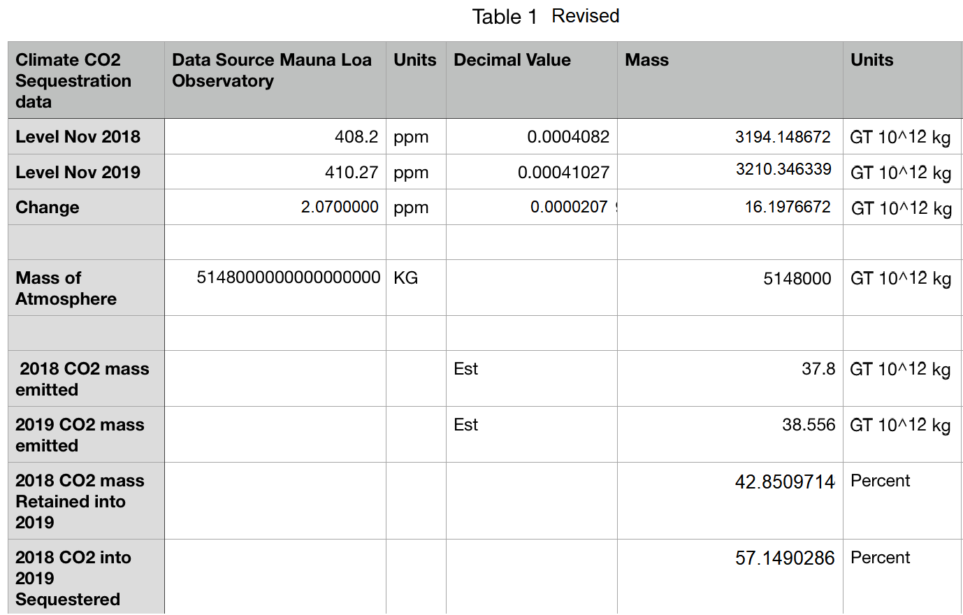
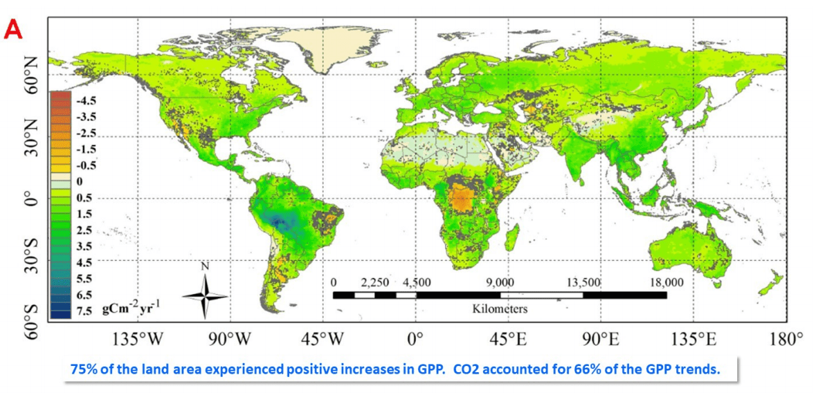




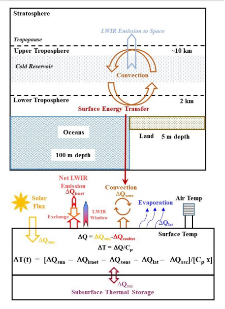
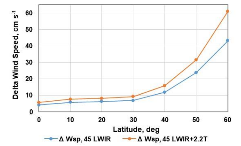
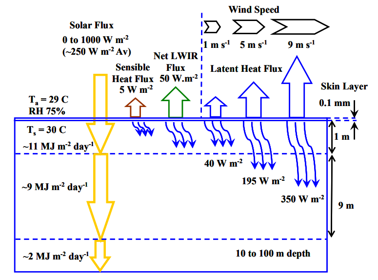

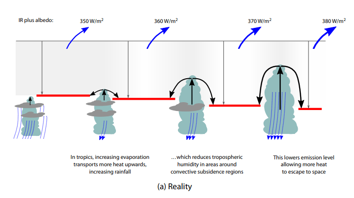
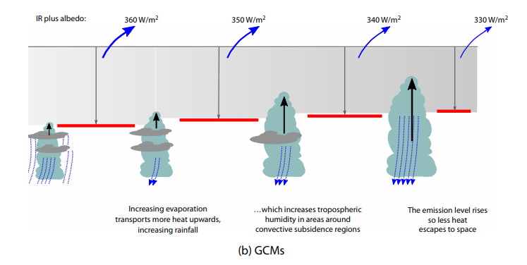
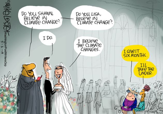

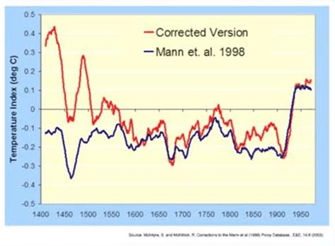

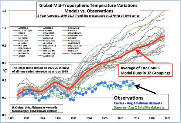




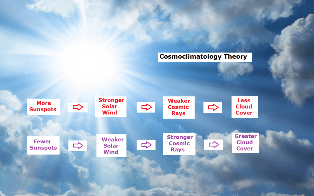
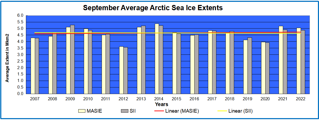


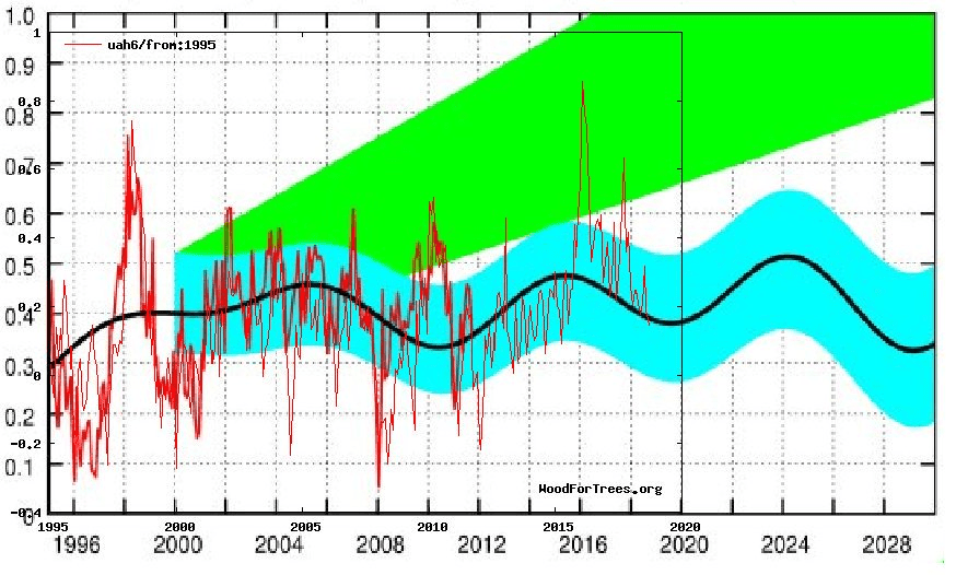


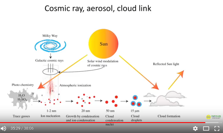

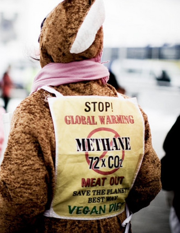

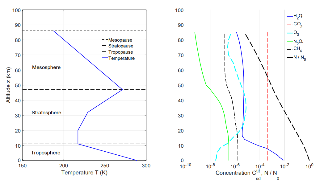


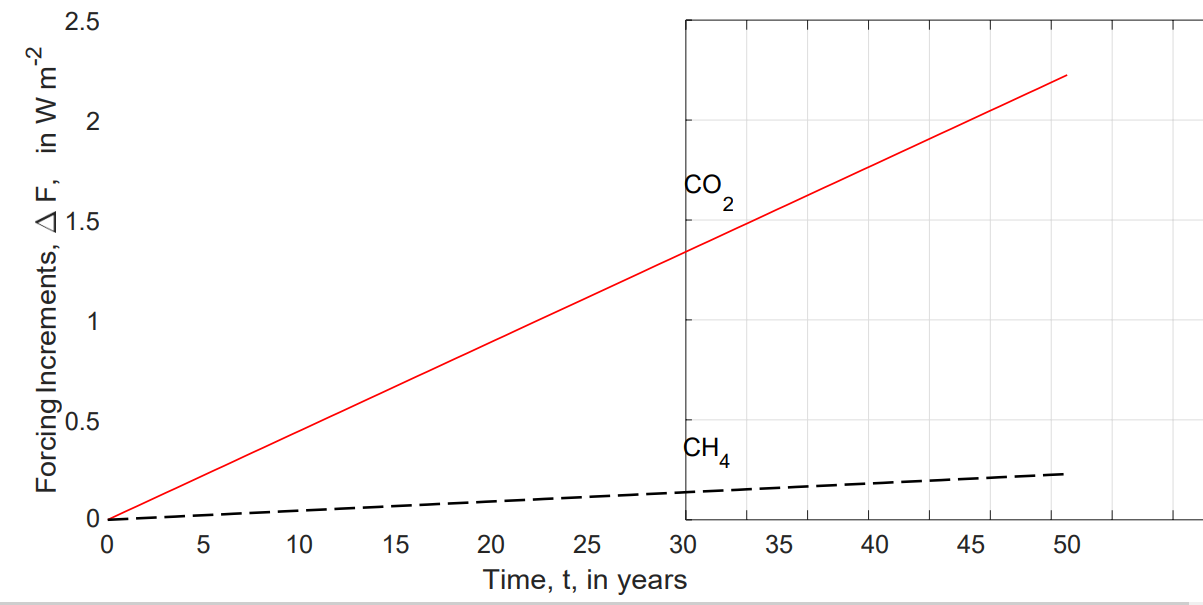


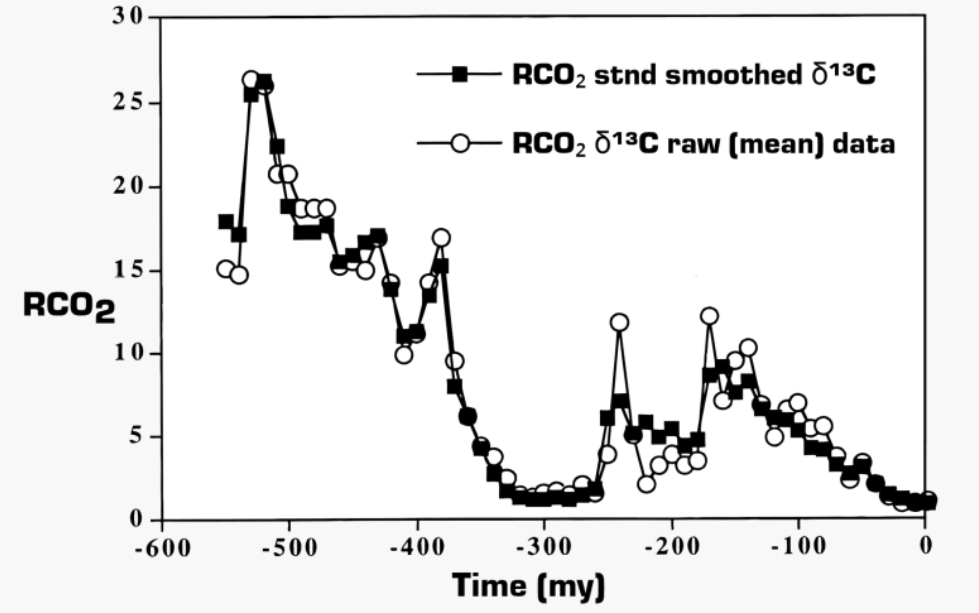

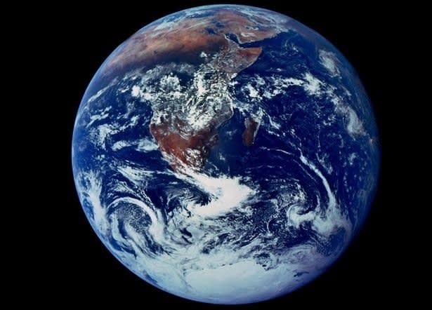
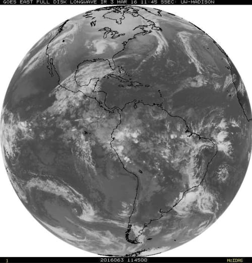
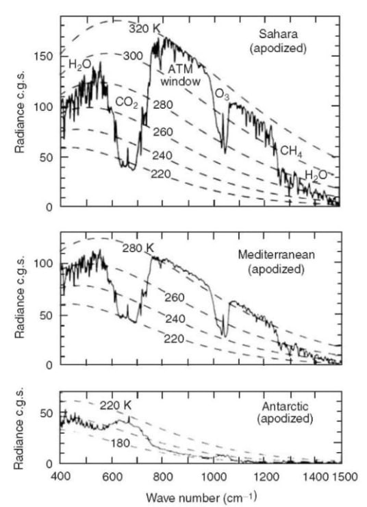
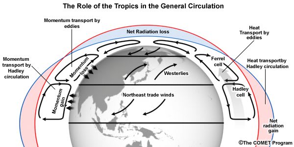


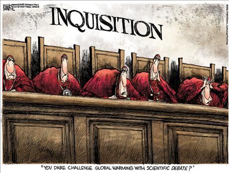

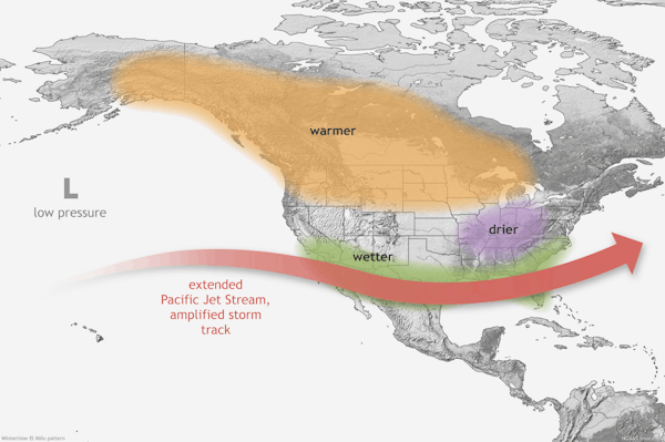
 Other scientists are more interested in the truth than in hype. An example is this AGU publication by D.A Smeed et al.

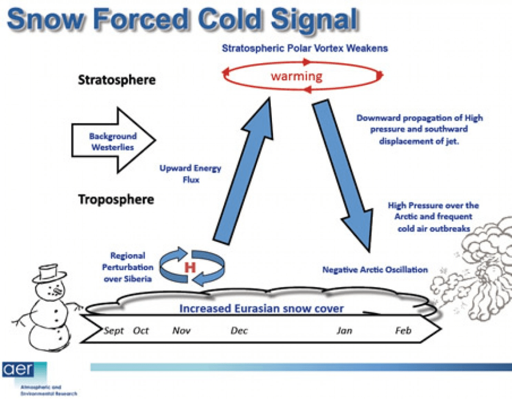


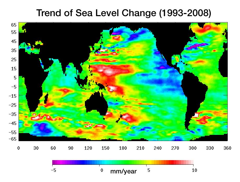
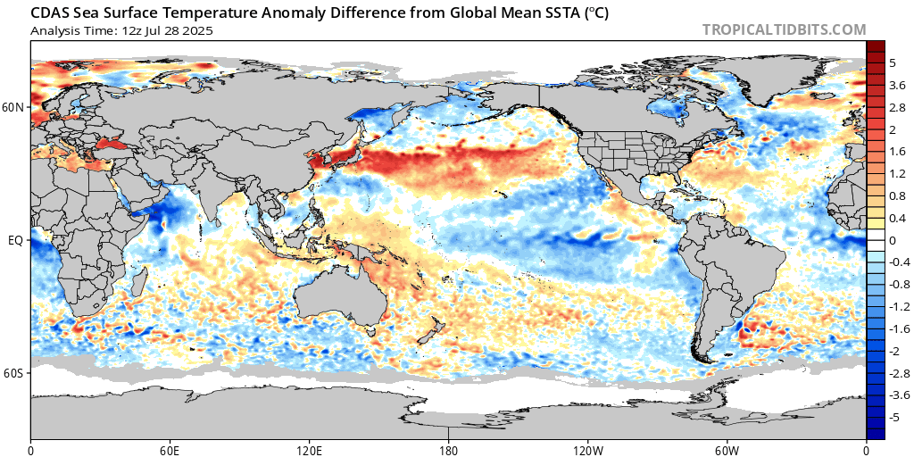
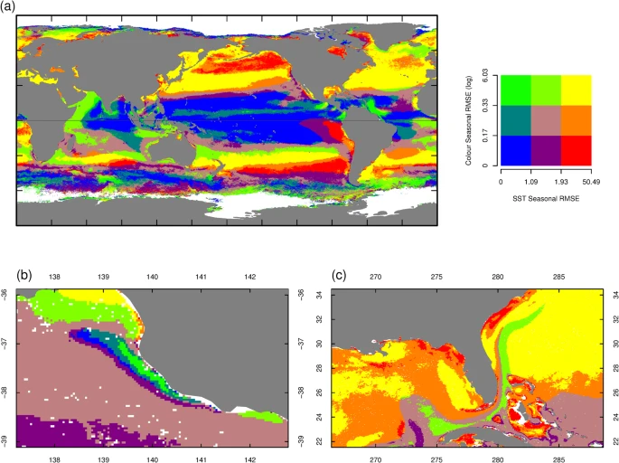

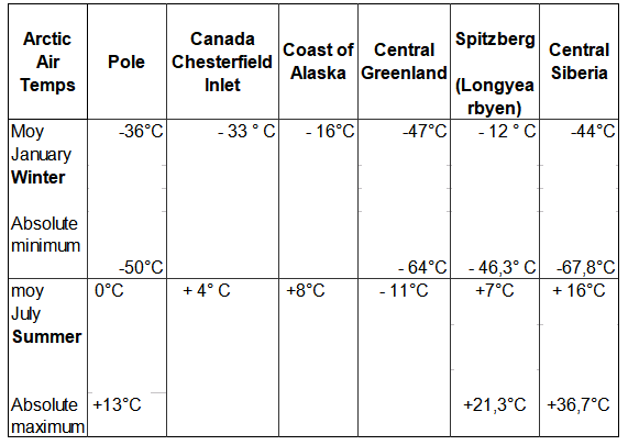
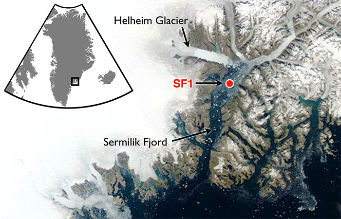

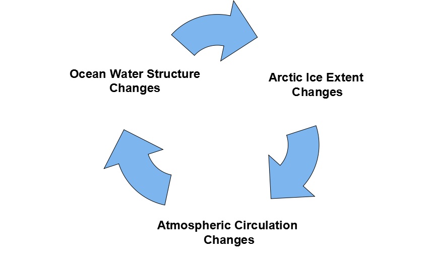

 Science Matters