It is often said we must rely on projections from computer simulations of earth’s climate since we have no other earth on which to experiment. That is not actually true since we have observations upon a number of planetary objects in our solar system that also have atmospheres.
This is brought home by a paper, published recently in the journal “Environment Pollution and Climate Change,” written by Ned Nikolov, a Ph.D. in physical science, and Karl Zeller, retired Ph.D. research meteorologist. (title is link to paper). H/T to Tallbloke for posting on this (here) along with comments by one of the authors.
New Insights on the Physical Nature of the Atmospheric Greenhouse Effect Deduced from an Empirical Planetary Temperature Model
Nikolov and Zeller have written before on this topic, but this paper takes advantage of data from recent decades of space exploration as well as improved observatories. It is thorough, educational and makes a convincing case that a planet’s surface temperatures can be predicted from two variables: distance from the sun, and the atmospheric mass. This post provides some excerpts and exhibits as a synopsis, hopefully to encourage reading the paper itself.
Abstract
A recent study has revealed that the Earth’s natural atmospheric greenhouse effect is around 90 K or about 2.7 times stronger than assumed for the past 40 years. A thermal enhancement of such a magnitude cannot be explained with the observed amount of outgoing infrared long-wave radiation absorbed by the atmosphere (i.e. ≈ 158 W m-2), thus requiring a re-examination of the underlying Greenhouse theory.
We present here a new investigation into the physical nature of the atmospheric thermal effect using a novel empirical approach toward predicting the Global Mean Annual near-surface equilibrium Temperature (GMAT) of rocky planets with diverse atmospheres. Our method utilizes Dimensional Analysis (DA) applied to a vetted set of observed data from six celestial bodies representing a broad range of physical environments in our Solar System, i.e. Venus, Earth, the Moon, Mars, Titan (a moon of Saturn), and Triton (a moon of Neptune).
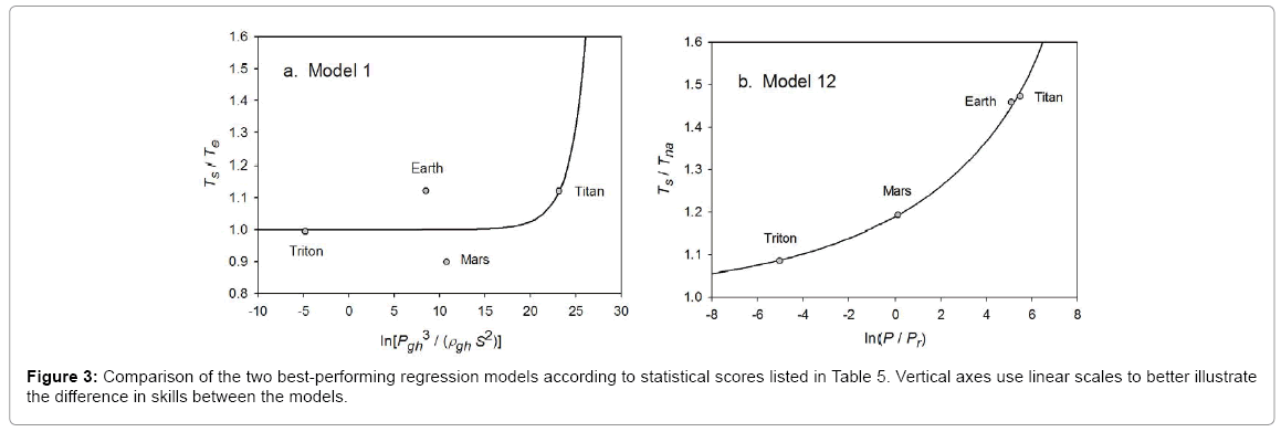
Twelve relationships (models) suggested by DA are explored via non-linear regression analyses that involve dimensionless products comprised of solar irradiance, greenhouse-gas partial pressure/density and total atmospheric pressure/density as forcing variables, and two temperature ratios as dependent variables. One non-linear regression model is found to statistically outperform the rest by a wide margin.

Venus is a furnace of a planet, with a noxious atmosphere bearing a pressure 90 times that on Earth. Courtesy NASA/JPL
Above: Venusian Atmosphere
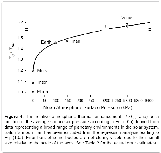
Our analysis revealed that GMATs of rocky planets with tangible atmospheres and a negligible geothermal surface heating can accurately be predicted over a broad range of conditions using only two forcing variables: top-of-the-atmosphere solar irradiance and total surface atmospheric pressure. The hereto discovered interplanetary pressure-temperature relationship is shown to be statistically robust while describing a smooth physical continuum without climatic tipping points.
This continuum fully explains the recently discovered 90 K thermal effect of Earth’s atmosphere. The new model displays characteristics of an emergent macro-level thermodynamic relationship heretofore unbeknown to science that has important theoretical implications. A key entailment from the model is that the atmospheric ‘greenhouse effect’ currently viewed as a radiative phenomenon is in fact an adiabatic (pressure-induced) thermal enhancement analogous to compression heating and independent of atmospheric composition. (my bold)

Earth Atmosphere Density and Temperature Profile
Consequently, the global down-welling long-wave flux presently assumed to drive Earth’s surface warming appears to be a product of the air temperature set by solar heating and atmospheric pressure. In other words, the so-called ‘greenhouse back radiation’ is globally a result of the atmospheric thermal effect rather than a cause for it. (my bold)
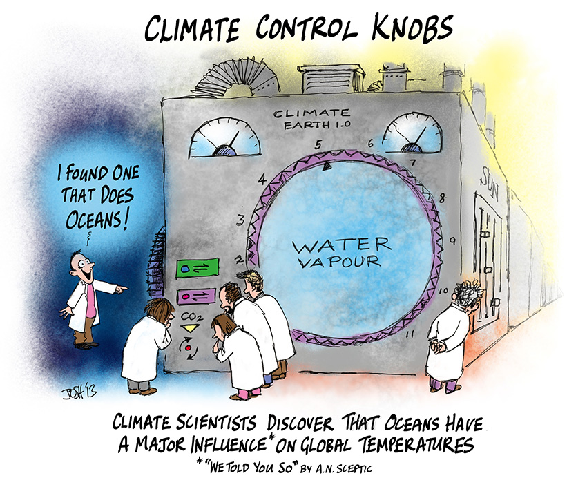
Our empirical model has also fundamental implications for the role of oceans, water vapour, and planetary albedo in global climate. Since produced by a rigorous attempt to describe planetary temperatures in the context of a cosmic continuum using an objective analysis of vetted observations from across the Solar System, these findings call for a paradigm shift in our understanding of the atmospheric ‘greenhouse effect’ as a fundamental property of climate.
The research effort demonstrates sound scientific research: data and sources are fully explained, the pattern analysis is replicable, and the conclusions set forth in a logical manner. Alternative hypotheses were explored and rejected in favor of one explaining observations to near perfection, and also showing applicability to other cases.
Equation (10a) implies that GMATs of rocky planets can be calculated as a product of two quantities: the planet’s average surface temperature in the absence of an atmosphere (Tna, K) and a nondimensional factor (Ea ≥ 1.0) quantifying the relative thermal effect of the atmosphere.
As an example of technical descriptions, consider how the paper describes issues relating to the calculation of Tna.
For bodies with tangible atmospheres (such as Venus, Earth, Mars, Titan and Triton), one must calculate Tna using αe=0.132 and ηe=0.00971, which assumes a Moon-like airless reference surface in accordance with our pre-analysis premise. For bodies with tenuous atmospheres (such as Mercury, the Moon, Calisto and Europa), Tna should be calculated from Eq. (4a) (or Eq. 4b respectively if S>0.15 W m-2 and/or Rg ≈ 0 W m-2) using the body’s observed values of Bond albedo αe and ground heat storage fraction ηe.
In the context of this model, a tangible atmosphere is defined as one that has significantly modified the optical and thermo-physical properties of a planet’s surface compared to an airless environment and/or noticeably impacted the overall planetary albedo by enabling the formation of clouds and haze. A tenuous atmosphere, on the other hand, is one that has not had a measurable influence on the surface albedo and regolith thermos-physical properties and is completely transparent to shortwave radiation.
The need for such delineation of atmospheric masses when calculating Tna arises from the fact that Eq. (10a) accurately describes RATEs of planetary bodies with tangible atmospheres over a wide range of conditions without explicitly accounting for the observed large differences in albedos (i.e., from 0.235 to 0.90) while assuming constant values of αe and ηe for the airless equivalent of these bodies. One possible explanation for this counterintuitive empirical result is that atmospheric pressure alters the planetary albedo and heat storage properties of the surface in a way that transforms these parameters from independent controllers of the global temperature in airless bodies to intrinsic byproducts of the climate system itself in worlds with appreciable atmospheres. In other words, once atmospheric pressure rises above a certain level, the effects of albedo and ground heat storage on GMAT become implicitly accounted for by Eq. (11). (my bold)
Significance
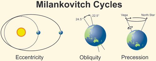
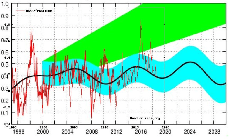
Equation (10b) describes the long-term (30 years) equilibrium GMATs of planetary bodies and does not predict inter-annual global temperature variations caused by intrinsic fluctuations of cloud albedo and/or ocean heat uptake. Thus, the observed 0.82 K rise of Earth’s global temperature since 1880 is not captured by our model, since this warming was likely not the result of an increased atmospheric pressure. Recent analyses of observed dimming and brightening periods worldwide [97-99] suggest that the warming over the past 130 years might have been caused by a decrease in global cloud cover and a subsequent increased absorption of solar radiation by the surface. Similarly, the mega shift of Earth’s climate from a ‘hothouse’ to an ‘icehouse’ evident in the sedimentary archives over the past 51 My cannot be explained by Eq. (10b) unless caused by a large loss of atmospheric mass and a corresponding significant drop in surface air pressure since the early Eocene.
Role of greenhouse gases from the new model perspective
Our analysis revealed a poor relationship between GMAT and the amount of greenhouse gases in planetary atmospheres across a broad range of environments in the Solar System (Figures 1-3 and Table 5). This is a surprising result from the standpoint of the current Greenhouse theory, which assumes that an atmosphere warms the surface of a planet (or moon) via trapping of radiant heat by certain gases controlling the atmospheric infrared optical depth [4,9,10]. The atmospheric opacity to LW radiation depends on air density and gas absorptivity, which in turn are functions of total pressure, temperature, and greenhouse-gas concentrations [9]. Pressure also controls the broadening of infrared absorption lines in individual gases. Therefore, the higher the pressure, the larger the infrared optical depth of an atmosphere, and the stronger the expected greenhouse effect would be. According to the present climate theory, pressure only indirectly affects global surface temperature through the atmospheric infrared opacity and its presumed constraint on the planet’s LW emission to Space [9,107].
The artificial decoupling between radiative and convective heat-transfer processes adopted in climate models leads to mathematically and physically incorrect solutions with regard to surface temperature. The LW radiative transfer in a real climate system is intimately intertwined with turbulent convection/advection as both transport mechanisms occur simultaneously. Since convection (and especially the moist one) is orders of magnitude more efficient in transferring energy than LW radiation [3,4], and because heat preferentially travels along the path of least resistance, a properly coupled radiative-convective algorithm of energy exchange will produce quantitatively and qualitatively different temperature solutions in response to a changing atmospheric composition than the ones obtained by current climate models. Specifically, a correctly coupled convective-radiative system will render the surface temperature insensitive to variations in the atmospheric infrared optical depth, a result indirectly supported by our analysis as well. This topic requires further investigation beyond the scope of the present study. (my bold)
The direct effect of atmospheric pressure on the global surface temperature has received virtually no attention in climate science thus far. However, the results from our empirical data analysis suggest that it deserves a serious consideration in the future.

How did Saturn’s moon Titan secure an atmosphere when no other moons in the solar system did? The answer lies largely in its size and location. Here, Titan as imaged in May 2005 by the Cassini spacecraft from about 900,000 miles away. Photo credit: Courtesy NASA/JPL/Space Science Institute
Physical nature of the atmospheric ‘greenhouse effect’
According to Eq. (10b), the heating mechanism of planetary atmospheres is analogous to a gravity-controlled adiabatic compression acting upon the entire surface. This means that the atmosphere does not function as an insulator reducing the rate of planet’s infrared cooling to space as presently assumed [9,10], but instead adiabatically boosts the kinetic energy of the lower troposphere beyond the level of solar input through gas compression. Hence, the physical nature of the atmospheric ‘greenhouse effect’ is a pressure-induced thermal enhancement independent of atmospheric composition. (my bold)
This mechanism is fundamentally different from the hypothesized ‘trapping’ of LW radiation by atmospheric trace gases first proposed in the 19th century and presently forming the core of the Greenhouse climate theory. However, a radiant-heat trapping by freely convective gases has never been demonstrated experimentally. We should point out that the hereto deduced adiabatic (pressure-controlled) nature of the atmospheric thermal effect rests on an objective analysis of vetted planetary observations from across the Solar System and is backed by proven thermodynamic principles, while the ‘trapping’ of LW radiation by an unconstrained atmosphere surmised by Fourier, Tyndall and Arrhenius in the 1800s was based on a theoretical conjecture. The latter has later been coded into algorithms that describe the surface temperature as a function of atmospheric infrared optical depth (instead of pressure) by artificially decoupling radiative transfer from convective heat exchange. Note also that the Ideal Gas Law (PV=nRT) forming the basis of atmospheric physics is indifferent to the gas chemical composition. (my bold)
Climate stability
Our semi-empirical model (Equations 4a, 10b and 11) suggests that, as long as the mean annual TOA solar flux and the total atmospheric mass of a planet are stationary, the equilibrium GMAT will remain stable. Inter-annual and decadal variations of global temperature forced by fluctuations of cloud cover, for example, are expected to be small compared to the magnitude of the background atmospheric warming because of strong negative feedbacks limiting the albedo changes. This implies a relatively stable climate for a planet such as Earth absent significant shifts in the total atmospheric mass and the planet’s orbital distance to the Sun. Hence, planetary climates appear to be free of tipping points, i.e., functional states fostering rapid and irreversible changes in the global temperature as a result of hypothesized positive feedbacks thought to operate within the system. In other words, our results suggest that the Earth’s climate is well buffered against sudden changes.
The hypothesis that a freely convective atmosphere could retain (trap) radiant heat due its opacity has remained undisputed since its introduction in the early 1800s even though it was based on a theoretical conjecture that has never been proven experimentally. It is important to note in this regard that the well-documented enhanced absorption of thermal radiation by certain gases does not imply an ability of such gases to trap heat in an open atmospheric environment. This is because, in gaseous systems, heat is primarily transferred (dissipated) by convection (i.e., through fluid motion) rather than radiative exchange. (my bold)
If gases of high LW absorptivity/emissivity such as CO2, methane and water vapor were indeed capable of trapping radiant heat, they could be used as insulators. However, practical experience has taught us that thermal radiation losses can only be reduced by using materials of very low IR absorptivity/emissivity and correspondingly high thermal reflectivity such as aluminum foil. These materials are known among engineers at NASA and in the construction industry as radiant barriers [129]. It is also known that high-emissivity materials promote radiative cooling. Yet, all climate models proposed since 1800s were built on the premise that the atmosphere warms Earth by limiting radiant heat losses of the surface through to the action of IR absorbing gases aloft.
If a trapping of radiant heat occurred in Earth’s atmosphere, the same mechanism should also be expected to operate in the atmospheres of other planetary bodies. Thus, the Greenhouse concept should be able to mathematically describe the observed variation of average planetary surface temperatures across the Solar System as a continuous function of the atmospheric infrared optical depth and solar insolation. However, to our knowledge, such a continuous description (model) does not exist.
Summary
The planetary temperature model consisting of Equations (4a), (10b), (11) has several fundamental theoretical implications, i.e.,
• The ‘greenhouse effect’ is not a radiative phenomenon driven by the atmospheric infrared optical depth as presently believed, but a pressure-induced thermal enhancement analogous to adiabatic heating and independent of atmospheric composition;
• The down-welling LW radiation is not a global driver of surface warming as hypothesized for over 100 years but a product of the near-surface air temperature controlled by solar heating and atmospheric pressure;
• The albedo of planetary bodies with tangible atmospheres is not an independent driver of climate but an intrinsic property (a byproduct) of the climate system itself. This does not mean that the cloud albedo cannot be influenced by external forcing such as solar wind or galactic cosmic rays. However, the magnitude of such influences is expected to be small due to the stabilizing effect of negative feedbacks operating within the system. This novel understanding explains the observed remarkable stability of planetary albedos;
• The equilibrium surface temperature of a planet is bound to remain stable (i.e., within ± 1 K) as long as the atmospheric mass and the TOA mean solar irradiance are stationary. Hence, Earth’s climate system is well buffered against sudden changes and has no tipping points;
• The proposed net positive feedback between surface temperature and the atmospheric infrared opacity controlled by water vapor appears to be a model artifact resulting from a mathematical decoupling of the radiative-convective heat transfer rather than a physical reality.

Update July 13, 2017
Michael Lewis pointed to a link on this subject in his comment below. Reading again the discussion thread, I appreciated again this point by point response from Kristian to Tim Folkerts so I am adding it to the post. (To be clear, T_e means emission temperature (same as Tna in the article above, while T_s means surface temperature.)
Kristian says:
August 4, 2016 at 9:24 AM
Tim Folkerts says, August 3, 2016 at 3:33 PM:
“In any case, it seems we both agree that the atmosphere has some warming effect.”
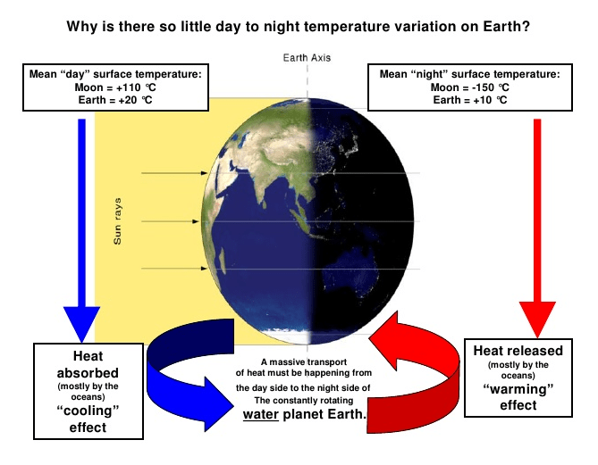
That’s quite obvious. You only need to compare Earth’s T_s with the Moon’s.
“I agree that the mass itself plays a role. Mass creates thermal inertia to even out temperature swings. The mass of the atmosphere (and oceans) also allows convection to carry energy from warmer areas to cooler areas, which further reduces variations. By themselves, these could do no more than bring T_s UP TOWARD T_e.”
True.
“I see no physics that would explain mass itself raising T_s ABOVE T_e.”
Just as the radiative properties of gaseous molecules are also not able – all by themselves – to raise a planet’s T_s above its T_e. No, both mass and radiative properties are needed.
“To get above T_e we need something to change the outgoing thermal radiation, eg GHGs at a high enough altitude to be significantly cooler than the surface.”
Yes, but then we also need an air column above the solar-heated surface that can have such a “high enough altitude” in the first place. We also need that altitude to be cooler on average than the surface. IOW, we need mass. A certain gas density/pressure (molecular interaction). And we need fluid dynamics.
“So the key factor is ALTITUDE here (with some definite dependence of the concentrations of the GHGs as well).”
No. There is no dependence on the CONCENTRATION/CONTENT of IR-active constituents in an atmosphere. An atmosphere definitely needs to be IR active (although it’s evidently not enough) for a planet’s T_s to become higher than its T_e. It also needs to be IR active to be able to adequately rid itself of its absorbed energy from the surface (radiatively AND non-radiatively transferred) and directly from the Sun. But once it’s IR active, there is no dependence on the degree of activity. Because then the atmosphere has become stably convectively operative. And all that matters from then on is atmospheric MASS and SOLAR INPUT (TSI and global albedo).
“You say that atmospheric mass seems to force. Do you think that mass alone without GHGs could force temperatures higher than T_e?”
No. Just like “GHGs” alone could also not force T_s higher than T_e. You need both.
* * *
So I say: There IS a “GHE”. But it’s ultimately massively caused. The radiative properties are simply a tool. A means to an end. And there definitely ISN’T an “anthropogenically enhanced GHE” (AGW). It cannot happen.
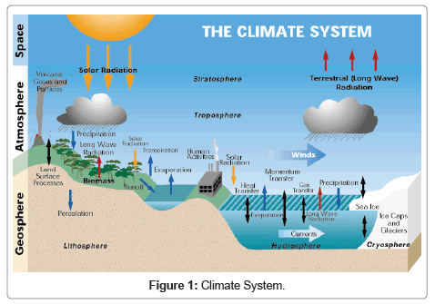
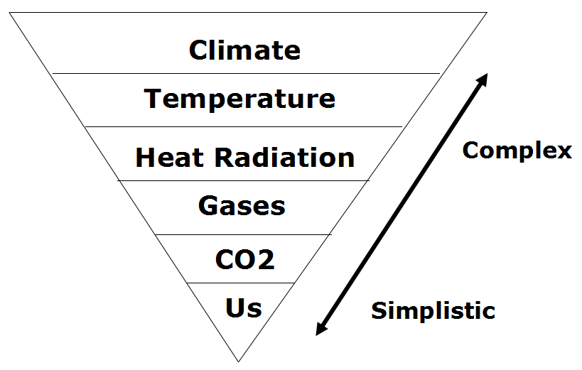
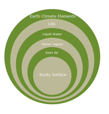 Thanks to No Tricks Zone for posting work (here) by Dr. Dai Davies of Canberra. In his writing I found a fine summary paradigm leading to the image above. This post presents a scientifically rigorous view of our planetary climate system, starting with an airless rocky surface and then conceptually adding the dynamic elements in layers. The text below with my bolds and images comes from Energy and Atmosphere by Dr. Dai Davies of University of Canberra, Website: http://brindabella.id.au/climarc/.


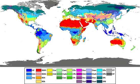
 Fortunately we have a well-established framework classifying climate zones based upon temperature and precipitation patterns. And researchers have addressed this question in this paper: Using the Köppen classification to quantify climate variation and change: An example for 1901–2010 By Deliang Chen and Hans Weiteng Chen Department of Earth Sciences, University of Gothenburg, Sweden