Many have noticed that recent speeches written for child activist Greta Thunberg are basing the climate “emergency” on the rapidly closing “carbon budget”. This post aims to summarize how alarmists define the so-called carbon budget, and why their claims to its authority are spurious. In the text and at the bottom are links to websites where readers can access both the consensus science papers and the analyses showing the flaws in the carbon budget notion. Excerpts are in italics with my bolds.

The 2019 update on the Global Carbon Budget was reported at Future Earth article entitled Global Carbon Budget Estimates Global CO2 Emissions Still Rising in 2019. The results were published by the Global Carbon Project in the journals Nature Climate Change, Environmental Research Letters, and Earth System Science Data. Excerpts below in italics with my bolds.

History of Growing CO2 Emissions

“Carbon dioxide emissions must decline sharply if the world is to meet the ‘well below 2°C’ mark set out in the Paris Agreement, and every year with growing emissions makes that target even more difficult to reach,” said Robbie Andrew, a Senior Researcher at the CICERO Center for International Climate Research in Norway.

Global emissions from coal use are expected to decline 0.9 percent in 2019 (range: -2.0 percent to +0.2 percent) due to an estimated 10 percent fall in the United States and a 10 percent fall in Europe, combined with weak growth in coal use in China (+0.8 percent) and India (+2 percent).

 

Shifting Mix of Fossil Fuel Consumption

“The weak growth in carbon dioxide emissions in 2019 is due to an unexpected decline in global coal use, but this drop is insufficient to overcome the robust growth in natural gas and oil consumption,” said Glen Peters, Research Director at CICERO.

“Global commitments made in Paris in 2015 to reduce emissions are not yet being matched by proportionate actions,” said Peters. “Despite political rhetoric and rapid growth in low carbon technologies such as solar and wind power, electric vehicles, and batteries, global fossil carbon dioxide emissions are likely to be more than four percent higher in 2019 than in 2015 when the Paris Agreement was adopted.”

“Compared to coal, natural gas is a cleaner fossil fuel, but unabated natural gas merely cooks the planet more slowly than coal,” said Peters. “While there may be some short-term emission reductions from using natural gas instead of coal, natural gas use needs to be phased out quickly on the heels of coal to meet ambitious climate goals.”

Oil and gas use have grown almost unabated in the last decade. Gas use has been pushed up by declines in coal use and increased demand for gas in industry. Oil is used mainly to fuel personal transport, freight, aviation and shipping, and to produce petrochemicals.

“This year’s Carbon Budget underscores the need for more definitive climate action from all sectors of society, from national and local governments to the private sector,” said Amy Luers, Future Earth’s Executive Director. “Like the youth climate movement is demanding, this requires large-scale systems changes – looking beyond traditional sector-based approaches to cross-cutting transformations in our governance and economic systems.”

Burning gas emits about 40 percent less CO2 than coal per unit energy, but it is not a zero-carbon fuel. While CO2 emissions are likely to decline when gas displaces coal in electricity production, Global Carbon Project researchers say it is only a short-term solution at best. All CO2 emissions will need to decline rapidly towards zero.

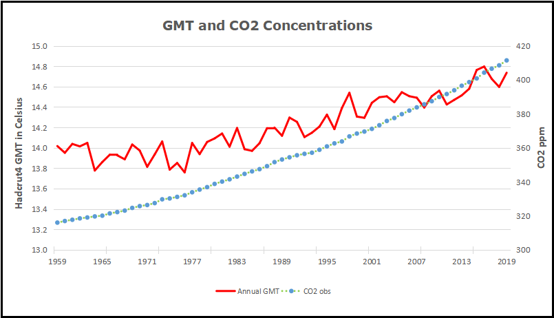
The Premise: Rising CO2 Emissions Cause Global Warming

Atmospheric CO2 concentration is set to reach 410 ppm on average in 2019, 47 percent above pre-industrial levels.

Glen Peters on the carbon budget and global carbon emissions is a Future of Earth interview explaining the Carbon Budget notion. Excerpts in italics with my bolds.

In many ways, the global carbon budget is like any other budget. There’s a maximum amount we can spend, and it must be allocated to various countries and various needs. But how do we determine how much carbon each country can emit? Can developing countries grow their economies without increasing their emissions? And if a large portion of China’s emissions come from products made for American and European consumption, who’s to blame for those emissions? Glen Peters, Research Director at the Center for International Climate Research (CICERO) in Oslo, explains the components that make up the carbon budget, the complexities of its calculation, and its implications for climate policy and mitigation efforts. He also discusses how emissions are allocated to different countries, how emissions are related to economic growth, what role China plays in all of this, and more.

The carbon budget generally has two components: the source component, so what’s going into the atmosphere; and the sink component, so the components which are more or less going out of the atmosphere.

So in terms of sources, we have fossil fuel emissions; so we dig up coal, oil, and gas and burn them and emit CO2. We have cement, which is a chemical reaction, which emits CO2. That’s sort of one important component on the source side. We also have land use change, so deforestation. We’re chopping down a lot of trees, burning them, using the wood products and so on. And then on the other side of the equation, sort of the sink side, we have some carbon coming back out in a sense to the atmosphere. So the land sucks up about 25% of the carbon that we put into the atmosphere and the ocean sucks up about 25%. So for every ton we put into the atmosphere, then only about half a ton of CO2 remains in the atmosphere. So in a sense, the oceans and the land are cleaning up half of our mess, if you like.

The other half just stays in the atmosphere. Half a ton stays in the atmosphere; the other half is cleaned up. It’s that carbon that stays in the atmosphere which is causing climate change and temperature increases and changes in precipitation and so on.

The carbon budget is like a balance, so you have something coming in and something going out, and in a sense by mass balance, they have to equal. So if we go out and we take an estimate of how much carbon have we emitted by burning fossil fuels or by chopping down forests and we try and estimate how much carbon has gone into the ocean or the land, then we can measure quite well how much carbon is in the atmosphere. So we can add all those measurements together and then we can compare the two totals — they should equal. But they don’t equal. And this is sort of part of the science, if we overestimated emissions or if we over or underestimated the strength of the land sink or the oceans or something like that. And we can also cross check with what our models say.

My Comment:

Several things are notable about the carbon cycle diagram from GCP. It claims the atmosphere adds 18 GtCO2 per year and drives Global Warming. Yet estimates of emissions from burning fossil fuels and from land use combined range from 36 to 45 GtCO2 per year, or +/- 4.5. The uptake by the biosphere and ocean combined range from 16 to 25 GtCO2 per year, also +/- 4.5. The uncertainty on emissions is 11% while the natural sequestration uncertainty is 22%, twice as much.

Furthermore, the fluxes from biosphere and ocean are both presented as balanced with no error range. The diagram assumes the natural sinks/sources are not in balance, but are taking more CO2 than they release. IPCC reported: Gross fluxes generally have uncertainties of more than +/- 20%. (IPCC AR4WG1 Figure 7.3.) Thus for land and ocean the estimates range as follows:

Land: 440, with uncertainty between 352 and 528, a range of 176
Ocean: 330, with uncertainty between 264 and 396, a range of 132
Nature: 770, with uncertainty between 616 and 924, a range of 308

So the natural flux uncertainty is 7.5 times the estimated human emissions of 41 GtCO2 per year.

For more detail see CO2 Fluxes, Sources and Sinks and Who to Blame for Rising CO2?

The Fundamental Flaw: Spurious Correlation

Beyond the uncertainty of the amounts is a method error in claiming rising CO2 drives temperature changes. For this discussion I am drawing on work by chaam jamal at her website Thongchai Thailand. A series of articles there explain in detail how the mistake was invented and why it is faulty. A good starting point is The Carbon Budgets of Climate Science. Below is my attempt at a synopsis from her writings with excerpts in italics and my bolds.

Simplifying Climate to a Single Number

Carbon budget accounting is based on the TCRE (Transient Climate Response to Cumulative Emissions). It is derived from the observed correlation between temperature and cumulative emissions. A comprehensive explanation of an application of this relationship in climate science is found in the IPCC SR 15 2018. This IPCC description is quoted below in paragraphs #1 to #7 where the IPCC describes how climate science uses the TCRE for climate action mitigation of AGW in terms of the so called the carbon budget. Also included are some of difficult issues in carbon budget accounting and the methods used in their resolution.

It has long been recognized that the climate sensitivity of surface temperature to the logarithm of atmospheric CO2 (ECS), which lies at the heart of the anthropogenic global warming and climate change (AGW) proposition, was a difficult issue for climate science because of the large range of empirical values reported in the literature and the so called “uncertainty problem” it implies.

The ECS uncertainty issue was interpreted in two very different ways. Climate science took the position that ECS uncertainty implies that climate action has to be greater than that implied by the mean value of ECS in order to ensure that higher values of ECS that are possible will be accommodated while skeptics argued that the large range means that we don’t really know. At the same time skeptics also presented convincing arguments against the assumption that observed changes in atmospheric CO2 concentration can be attributed to fossil fuel emissions.

A breakthrough came in 2009 when Damon Matthews, Myles Allen, and a few others almost simultaneously published almost identical papers reporting the discovery of a “near perfect” correlation (ρ≈1) between surface temperature and cumulative emissions {2009: Matthews, H. Damon, et al. “The proportionality of global warming to cumulative carbon emissions” Nature 459.7248 (2009): 829}. They had found that, irrespective of the timing of emissions or of atmospheric CO2 concentration, emitting a trillion tonnes of carbon will cause 1.0 – 2.1 C of global warming. This linear regression coefficient corresponding with the near perfect correlation between cumulative warming and cumulative emissions (note: temperature=cumulative warming), initially described as the Climate Carbon Response (CCR) was later termed the Transient Climate Response to Cumulative Emissions (TCRE).

Initially a curiosity, it gained in importance when it was found that it was in fact predicting future temperatures consistent with model predictions. The consistency with climate models was taken as a validation of the new tool and the TCRE became integrated into the theory of climate change. However, as noted in a related post the consistency likely derives from the assumption that emissions accumulate in the atmosphere.

Thereafter the TCRE became incorporated into the foundation of climate change theory particularly so in terms of its utility in the construction of carbon budgets for climate action plans for any given target temperature rise, an application for which the TCRE appeared to be tailor made. Most importantly, it solved or perhaps bypassed the messy and inconclusive uncertainty issue in ECS climate sensitivity that remained unresolved. The importance of this aspect of the TCRE is found in the 2017 paper “Beyond Climate Sensitivity” by prominent climate scientist Reto Knutti where he declared that the TCRE metric should replace the ECS as the primary tool for relating warming to human caused emissions {2017: Knutti, Reto, Maria AA Rugenstein, and Gabriele C. Hegerl. “Beyond equilibrium climate sensitivity.” Nature Geoscience 10.10 (2017): 727}. The anti ECS Knutti paper was not only published but received with great fanfare by the journal and by the climate science community in general.

The TCRE has continued to gain in importance and prominence as a tool for the practical application of climate change theory in terms of its utility in the construction and tracking of carbon budgets for limiting warming to a target such as the Paris Climate Accord target of +1.5C above pre-industrial. {Matthews, H. Damon. “Quantifying historical carbon and climate debts among nations.” Nature climate change 6.1 (2016): 60}. A bibliography on the subject of TCRE carbon budgets is included below at the end of this article (here).

However, a mysterious and vexing issue has arisen in the practical matter of applying and tracking TCRE based carbon budgets. The unsolved matter in the TCRE carbon budget is the remaining carbon budget puzzle {Rogelj, Joeri, et al. “Estimating and tracking the remaining carbon budget for stringent climate targets.” Nature 571.7765 (2019): 335-342}. It turns out that midway in the implementation of a carbon budget, the remaining carbon budget computed by subtraction does not match the TCRE carbon budget for the latter period computed directly using the Damon Matthews proportionality of temperature with cumulative emissions for that period. As it turns out, the difference between the two estimates of the remaining carbon budget has a rational explanation in terms of the statistics of a time series of cumulative values of another time series described in a related post

It is shown that a time series of the cumulative values of another time series has neither time scale nor degrees of freedom and that therefore statistical properties of this series can have no practical interpretation.

It is demonstrated with random numbers that the only practical implication of the “near perfect proportionality” correlation reported by Damon Matthews is that the two time series being compared (annual warming and annual emissions) tend to have positive values. In the case of emissions we have all positive values, and during a time of global warming, the annual warming series contains mostly positive values. The correlation between temperature (cumulative warming) and cumulative emissions derives from this sign bias as demonstrated with random numbers with and without sign bias.

Figure 4: Random Numbers without Sign Bias

Figure 5: Random Numbers with Sign Bias

The sign bias explains the correlation between cumulative values of time series data and also the remaining carbon budget puzzle. It is shown that the TCRE regression coefficient between these time series of cumulative values derives from the positive value bias in the annual warming data. Thus, during a period of accelerated warming, the second half of the carbon budget period may contain a higher percentage of positive values for annual warming and it will therefore show a carbon budget that exceeds the proportional budget for the second half computed from the full span regression coefficient that is based on a lower bias for positive values.

In short, the bias for positive annual warming is highest for the second half, lowest for the first half, and midway between these two values for the full span – and therein lies the simple statistics explanation of the remaining carbon budget issue that climate science is trying to solve in terms of climate theory and its extension to Earth System Models. The Millar and Friedlingstein 2018 paper is yet another in a long line of studies that ignore the statistical issues the TCRE correlation and instead try to explain its anomalous behavior in terms of climate theory whereas in fact their explanation lies in statistical issues that have been overlooked by these young scientists.

The fundamental problem with the construction of TCRE carbon budgets and their interpretation in terms of climate action is that the TCRE is a spurious correlation that has no interpretation in terms of a relationship between emissions and warming. Complexities in these carbon budgets such as the remaining carbon budget are best understood in these terms and not in terms of new and esoteric variables such as those in earth system models.

Footnote:

An independent study by Jamal Munshi come to a similar conclusion. Climate Sensitivity and the Responsiveness of Temperature to Atmospheric CO2

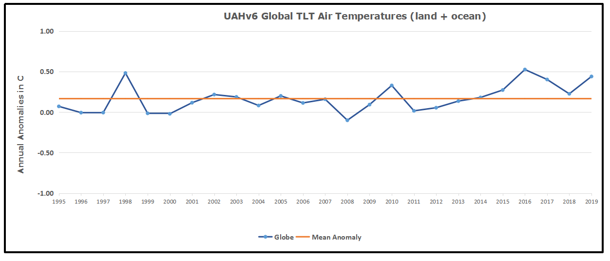
Detrended correlation analysis of global mean temperature observations and model projections are compared in a test for the theory that surface temperature is responsive to atmospheric CO2 concentration in terms of GHG forcing of surface temperature implied by the Climate Sensitivity parameter ECS. The test shows strong evidence of GHG forcing of warming in the theoretical RCP8.5 temperature projections made with CMIP5 forcings. However, no evidence of GHG forcing by CO2 is found in observational temperatures from four sources including two from satellite measurements. The test period is set to 1979-2018 so that satellite data can be included on a comparable basis. No empirical evidence is found in these data for a climate sensitivity parameter that determines surface temperature according to atmospheric CO2 concentration or for the proposition that reductions in fossil fuel emissions will moderate the rate of warming.

Postscript on Spurious Correlations

I am not a climate, environment, geology, weather, or physics expert. However, I am an expert on statistics. So, I recognize bad statistical analysis when I see it. There are quite a few problems with the use of statistics within the global warming debate. The use of Gaussian statistics is the first error. In his first movie Gore used a linear regression of CO2 and temperature. If he had done the same regression using the number of zoos in the world, or the worldwide use of atomic energy, or sunspots, he would have the same result. A linear regression by itself proves nothing.–Dan Ashley · PhD statistics, PhD Business, Northcentral University