Time Rethinks Greta

Now that’s more like it! (Though I worry it might be photoshopped.)
Now that’s more like it! (Though I worry it might be photoshopped.)

I have often written that prudent policymakers recognize the future will include periods both warmer and cooler than the present, and cold is the greater threat to human life and prosperity. Thus, government priorities should be to invest in affordable reliable energy and robust infrastructure. A recent article gets the importance of energy abundance, and makes many lucid points about climate policy failures, even while accepting uncritically some mistaken suppositions about the issue and what can be done about it.
Matt Frost published an article at The New Atlantis After Climate Despair. Excerpts in italics with my bolds, some images and comments.
The dream of a global conversion to austerity has failed to stop climate change. Energy abundance is our best hope for living well with warming — and reversing it.
Overview
Each of us constitutes a link between the past and the future, and we share a human need to participate in the life of something that perdures beyond our own years. This is the conservationist — and arguably the conservative — argument for combating climate change: Our descendants, who will have a great deal in common with us, ought to be able to enjoy conditions similar to those that permitted us and our forebears to thrive.
But the dominant narrative of climate change, though it claims to be aimed at protecting future generations, in fact leaves little room for continuity. Preventing more than 1.5 degrees Celsius of warming above the nineteenth-century baseline, the latest aim of the Intergovernmental Panel on Climate Change (IPCC), will, as they put it, require “rapid, far-reaching and unprecedented changes in all aspects of society.”
Only a vanishingly unlikely set of coordinated global actions — an extraordinary political breakthrough — can save us from what the most pessimistic media portrayals describe as “catastrophe,” “apocalypse,” and the “end of civilization.”
Only by changing our entire energy system and social order can we preserve the continuity of our biosphere. And so climate politics has become the art of the impossible: a cycle of increasingly desperate exhortations to impracticable action, presumably in hopes of inspiring at least some half-measures. Understandably, many despair, while others deny that there is a problem, or at least that any solution is possible.
But we are not condemned to a choice between despair and denial. Instead, we must prepare for a future in which we have temporarily failed to arrest climate change — while ensuring that human civilization stubbornly persists, and thrives. Rather than prescribing global austerity, reducing our energy usage and thereby limiting our options for adaptation, we should pursue energy abundance. Only in a high-energy future can we hope eventually to reduce the atmosphere’s carbon, through sequestration and by gradually replacing fossil fuels with low-carbon alternatives.

It is time to acknowledge that catastrophism has failed to bring about the global political breakthrough the climate establishment dreams of, and will not succeed in time to avert serious warming. Instead of despairing over a forever-deferred dream of austerity, our resources would be better spent now on investing in potential technological breakthroughs to reduce atmospheric carbon, and our political imagination better put toward preparing for a future of ever more abundant energy.
[Frost could have added that human flourishing has always occured in warmer, rather than colder times. Our Modern Warm Period was preceded by Medieval Warming, before that by Roman Warming, and earlier Minoan Warming. Each period was cooler than the previous, so the overall trend in our interglacial is downward. Ensuring favorable conditions for future generations means protecting against the ravages of frosty times. (pun intended)]
The Futility of Dread
The bleak poll results may reflect a broad, if perhaps tacit, agreement that we have reached diminishing returns on dread. Even now that most Americans accept the dire predictions of scientists and journalists, their assent does not change the fact that we currently lack the institutional, technological, and moral resources to prevent further climate change in the near term. The lay public has been taught to regard stabilizing the climate as an all-or-nothing struggle against the encroachment of a dismal future.
The bar for success is set high enough that failure is now the rational expectation.
A common reaction to “there is no solution” is “then there is no problem.” No matter how persuasive the evidence of impending danger, most people find ways to dismiss or evade problems that appear insoluble. Attempting to build political support for impossible interventions by making ever more pessimistic predictions will not work; it will only leave us mired in gloom and impotence. This polarized fatalism will grow more extreme as opposing partisans, recognizing our dearth of practicable options, choose either glib denial or morbid brooding.

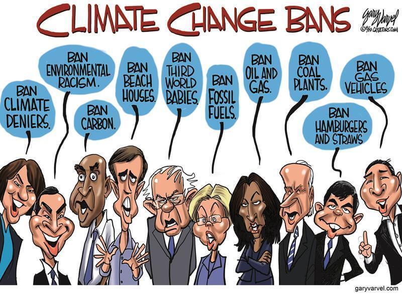
Entirely predictable Time Magazine declares Greta Person of the Year. Just like Big Brother she is watching.
Missing the Target
We will not stop global warming, at least in our lifetimes. This realization forces us to ask instead what would count as limiting warming enough to sustain our lives and our civilization through the disruption. There can be no single global answer to this question: Our ability to predict climate effects will always be limited, and what will count as acceptable warming to a Norwegian farmer enjoying a longer growing season will always be irreconcilable with that of a Miami resident fighting the sea to save his home. But because our leadership has approached climate change as a problem of coordinated global action, they have constructed quantitative waypoints around which to organize the debate.
Some news sources portrayed 2030 as an official deadline for avoiding climate catastrophe. It is worth noting that the report’s lead author, Myles Allen, has warned against this interpretation: “Please stop saying something globally bad is going to happen in 2030. Bad stuff is already happening and every half a degree of warming matters, but the IPCC does not draw a ‘planetary boundary’ at 1.5 degrees Celsius beyond which lie climate dragons.”

The extreme unlikelihood that we will meet the target of 1.5 degrees becomes even clearer when we notice that doing so requires that we not only cut emissions radically, but at the same time remove enormous volumes of carbon dioxide already emitted. The report estimates that a total of 100 billion tons must be removed by 2050. For comparison, the amount of carbon dioxide emitted globally from fossil fuels last year was around 37 billion tons.
Even were it possible to scale bioenergy and capture that quickly, doing so would have a major drawback: It would take up an immense amount of farmland. By one 2016 estimate, capturing enough carbon to meet even the 2-degree target by the end of the century could require devoting up to three million square miles of farmland to bioenergy crops — nearly the size of the contiguous United States.
[Frost seems not to realize the the 2C target, and more recently 1.5C are both rabbits pulled out of a magical activist hat. Economists have projected that future generations will be far wealthier than us, and only slightly less so should there be all the warming predicted from burning known carbon fuel reserves. Many dangers are based upon scenario RCP8.5 which is so unrealistic that some analysts say that models using it should be revised. Principled inaction is appropriate when threats are claimed without solid evidence.]
The Age of Overshoot
Expanding the climate options we allow ourselves to consider is easier said than done. The political and moral challenges are daunting. We will need to adapt to a warmer climate for perhaps decades to come, while at the same time preparing technological and policy solutions for a more distant future where we can finally claw our way back to lower levels of carbon and warming. At the same time, the stressors that a warmer climate will bring will be unequally felt across the globe, likely making our politics more divided and only dimming hopes for international coordination.

We must finally abandon the empty hope of imposing equitable austerity via globally coordinated government fiat.
Furthermore, as we adapt to a warmer climate, complacency will be tempting, since we will likely not experience a sudden decline in global quality of life or biodiversity, and may be able to avoid the most dire disruptions. Changes will be slow, with many unfolding on a generational time scale, and with dramatically different impacts among populations. The misery that climate change is likely to cause, or is already causing, will be difficult to distinguish from deprivation as we already know it — the people most harmed, that is, will be the poor, who are already most vulnerable to natural forces. Even if there is a distinct moment of irrecoverable failure, or a tipping point that triggers the worst feedback effects, most people might not notice until it has passed.
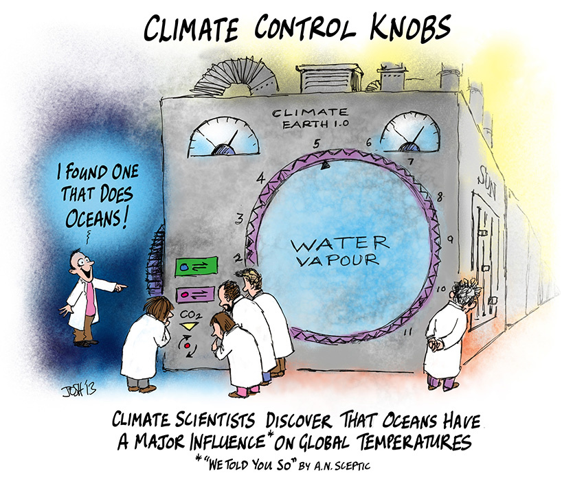
[His belief that CO2 is some kind of temperature control knob is touching, but naive and dangerous. H2O is actually earth’s thermostat, and we don’t have a dial for that either. Fortunately the climate system includes complex negative feedbacks which throughout history have kept both ice house and hot house eras from being permanent. Otherwise we would not be here to talk about it.]
The global failure to control emissions is not just a failure of political will or technological progress. Rather, it reflects the problem’s inherent resistance to unambiguous characterization. Different observers can all adopt different conceptions of the problem, many of which are not mutually exclusive but remain practically or politically irreconcilable.
For this reason, we will no more agree on some single new ethics than we will on the “correct” amount of atmospheric carbon dioxide.
Addressing the problem, then, must not mean the coordinated pursuit of a single solution but a perpetual process of decentralized negotiation and risk reduction. Our varied conceptions of climate change will never fully converge, and so the “correctness” of any approach is best evaluated not by whether it meets the latest IPCC target but by how well it affords broad political buy-in. Identifying alternatives to our current, failed approach to climate change requires identifying a more constructive set of ideas — practical, political, and sentimental. We will then be able to focus our resources on those interventions most likely to succeed.
[Among the failed solutions is the idea that modern societies can be powered with solar and wind energy. Not only is bioenergy land intensive (as noted above), so are these other renewables. Here is the map of UK showing the acreage required to power London without thermal generators.]

The gray area would be covered in wind farms, while the yellow area is needed for solar farms.
Austerity vs. Abundance
What should motivate our response to climate change is what got us into this mess in the first place: our desire for the abundance that energy technology affords. Energy is the commodity that allows us to protect ourselves from the ravages of nature and to live distinctly human lives, and many of the benefits we enjoy today were made possible by the exploitation of fossil energy. Our children should enjoy greater energy abundance than us, not less.
But the mainstream climate establishment — the government officials, researchers, advocates, and journalists who sustain the consensus agenda represented by the IPCC — is bent on austerity. They demand that we ration fossil energy consumption until zero-emission sources like wind and solar replace the fossil share of the global energy budget.
Discussions about climate change are also riddled with population anxiety. Lugubrious climate dread appears both as the idea that we should not inflict any more humans on this dying world and that we should not inflict this dying world on any more humans. For the most part, we no longer suffer from feverish speculation about runaway global population growth, since the population may peak anyway by the end of the century. Yet we still hear the old Malthusian idea that our limited energy resources will only be enough for everyone if there are fewer people to whom they must be handed out. Because the climate establishment views energy consumption as the problem, energy consumers must be on the negative side of the ledger — even if their welfare, or their grandchildren’s welfare, is supposed to be the good being protected.
An alternate framework based on abundance would engage each of us as participants in the flow of human history, as the forebears of unknown successors. It would complement even the doomsayers’ calls for taking expensive measures today, since the benefits of mitigating climate change would apply to more people as the population increases. The number of future occupants of our planet is, or should be, the salient variable in any calculation of the long-term costs and benefits of climate change mitigation and adaptation measures. We can’t know the economic return on any dollar we invest today in stabilizing the future climate, but we can model it as a function of, among other things, the number of our grandchildren’s grandchildren. Our climate approach should presuppose that we are the benefactors of a burgeoning future population, not the progenitors of an ascetic cult formed to dole out a dwindling stock of resources. New sources of carbon-free energy would offer more value to more people than whatever new levers of social control we might invent to enforce a worldwide carbon-rationing regime.
A stronger focus on human utility does not discount the non-human biosphere: When we evaluate the natural world for its beauty or its diversity, we are still expressing human values, and those values are part of the civilization we hope to carry forward in time. For instance, the desire to protect coral reefs, one of the first casualties of global warming, can increase as more people gain freedom from poverty, allowing them to see the reefs’ aesthetic and ecological benefits as worth spending resources to preserve.
An abundance framework is also aligned with our persistent human desire for comfort, and would lead us to reformulate our collective problem as one of scarcity, rather than prodigality. Instead of constraining our energy budget, we would look to a future in which a large, decarbonized energy capacity allows more people to enjoy the access to wealth and comfort that many of us take for granted. It would make little sense to leave cheap fossil energy underground in the name of future generations’ well-being, only to also leave those descendants an energy-constrained world full of incentives to drill. To remove those incentives, they will need abundant energy.
Obviously, meeting the energy demand of a high-growth world would require new sources of carbon-free power in amounts beyond the IPCC’s most optimistic scenarios. But we are already stuck hoping for a global political breakthrough. Technological breakthroughs are less far-fetched a solution. And a mass embrace of abundant energy is more realistic than sudden globally coordinated altruistic self-abnegation. Once we embrace abundance as a normative principle, it directs our attention and ambition toward the bets that, however long the odds, might actually pay off.
Embracing abundance means more than just a rhetorical or sentimental overhaul; it should change how we rank our policy and technology options. And gaining new energy sources would actually expand our options beyond the limited ones available to us now. Choosing abundance does not require that we first have all the answers for how to produce carbon-free energy, or how to reduce current levels of carbon dioxide. Rather, shifting our mindset from austerity to abundance will open up the political space necessary for imagining these answers and pursuing them.
In the near term, we must accept that expanding our political capacity to regulate carbon dioxide depends on driving down the cost of carbon-free energy. Penalizing fossil-energy use can encourage research and development of alternatives, but panic alone will not engender a new democratic mandate for costly restrictions on emissions. Cheap, low-carbon energy can be an alternative to bureaucratic rationing or socially enforced austerity. If we are stuck hoping for a breakthrough, let us hope for one that further emancipates us from want rather than one that more efficiently imposes it.
After Despair
We are stuck waiting for a breakthrough. The sort of breakthrough we await says much about who we are and where we hope to go. The consensus austerity view would have us hope for a moral breakthrough of penitential retrenchment. The abundance view would have us hope for a technological breakthrough to enable a flourishing future. One says that we have used too much energy, and our descendants should use less. The other implies that we have not devoted enough energy to capturing and storing carbon dioxide, and that we must leave our children and grandchildren as much energy capacity as possible to clean up our carbon waste.
Our mission must be to provide future generations with better technological alternatives than the ones currently on offer, which range from prohibitively expensive (like BECCS) to wildly reckless (like pumping sulfur dioxide into the stratosphere to block sunlight). We owe our descendants progress toward the long-deferred dream of energy “too cheap to meter,” as Lewis Strauss, chairman of the Atomic Energy Commission, famously said in 1954. We owe them the tools with which to dispose of the waste carbon they will inherit. We owe them a better sentimental investment than morbid despair about the future they will occupy.
Other policy approaches are less applicable to a strategic framework of energy abundance. “Weaning ourselves off nuclear energy,” as Senator Elizabeth Warren proposes, is a fatuous idea even within the austerity framework, if the risks of climate change are as dire as predicted. Replacing already online, zero-carbon generation with wind and solar plants that require carbon-emitting construction and infrastructure overhauls will only dig us deeper into debt. In an abundance framework, the proposal becomes even more misguided.
The policy measures we pursue in the near term should express the ethos of abundance and continuity. They should avoid emission cuts today that might limit wealth and technology options tomorrow. And they should set us up to take the best advantage of whatever breakthroughs, technological or political, we might be fortunate enough to see in the coming years.
Key Points
Global conversion to austerity is a lost cause.
Energy abundance is our best hope for the future.
We have always lived well when it warms.
When nature reverses and cools, we had better be ready.
Footnote: Since 1985 the band Opus has celebrated Life and access to energy (I’m sure they were referring to electrical power as well as personal mobility).
 Rich Lowry explains at NY Post Dems’ impeachment absurdities are making them look like the threat to democracy. Excerpts in italics with my bolds.
Summary:
The bottom line is that after tsk-tsking Trump for refusing to say in advance that he’d accept the outcome of the 2016 election, Democrats have steadfastly refused to truly accept the 2016 result, allegedly the work of the Russians, and now are signaling they won’t accept next year’s election, either, should they lose again.
With every day that passes, the Democrats risk a growing perception that they themselves are a threat to the 2020 election.
 Synopsis:
The Democrats believe that the 2020 election is too important to be left to the voters. It’s obvious that President Trump withheld defense aid to Ukraine to pressure its president to commit to the investigations that he wanted, an improper use of his power that should rightly be the focus of congressional investigation and hearings.
Where the Democrats have gotten tangled up is trying to find a justification that supports the enormous weight of impeaching and removing a president for the first time in our history.

They’ve cycled through different arguments. First, Trump’s offense was said to be a quid pro quo — a phrase cast aside for supposedly being too Latin for the public to understand. Then it was bribery, which has lost ground lately, presumably because of the inherent implausibility of the charge.
Now, the emphasis is on Trump’s invitation to the Ukrainians to “meddle” and “interfere” in our elections.

This is posited to be an ongoing threat. Nancy Pelosi said in her statement calling on the House to draft articles of impeachment: “Our democracy is what is at stake. The president leaves us no choice but to act, because he is trying to corrupt, once again, the election for his own benefit. The president has engaged in abuse of power undermining our national security and jeopardizing the integrity of our elections.”
House Judiciary Committee Chairman Jerry Nadler said on “Meet the Press” last weekend that Trump has to be impeached “for posing the considerable risk that he poses to the next election.” Asked if he thinks the 2020 election will be on the up-and-up, he said, “I don’t know. The president, based on his past performance, will do everything he can to make it not a fair election.”
The gravamen of this case is that the election is too crucial to allow the incumbent president of the United States, who is leading in key battleground states and has some significant chance of winning, to run. In fact, the integrity of the election is so at risk that the US Senate should keep the public from rendering a judgment on Trump’s first term or deciding between him and, say, his nemesis Joe Biden.

Of course, it’s possible to imagine a circumstance where a president would indeed present such a grave risk to our elections that he’d have to be removed. This is a reason that we have the impeachment process in the first place.
But what’s the real harm that Trump’s foolhardy Ukraine adventure presented?
Let’s say that Ukraine had, in response to Trump pressure, actually announced an investigation into Burisma, a shady company that had in the past been under investigation. What would have happened? Would Joe Biden have been forced from the race? Would his numbers have collapsed in Nevada and South Carolina, his best early states? Would his numbers have changed anywhere?
No, it’s not even clear there would have been any additional domestic political scrutiny of Hunter Biden’s lucrative arrangement with Burisma, an issue that is dogging the former vice president on the campaign trail anyway — because his son’s payday was so clearly inappropriate.
The bottom line is that after tsk-tsking Trump for refusing to say in advance that he’d accept the outcome of the 2016 election, Democrats have steadfastly refused to truly accept the 2016 result, allegedly the work of the Russians, and now are signaling they won’t accept next year’s election, either, should they lose again.

Given their druthers, Trump wouldn’t be an option for the voters. They are rushing their impeachment, in part, because they know that as November 2020 approaches, it becomes steadily less tenable to portray the man who wants to run in an election as the threat to democracy and the people who want to stop him as its champions.
With every day that passes, the Democrats risk a growing perception that they themselves are a threat to the 2020 election.


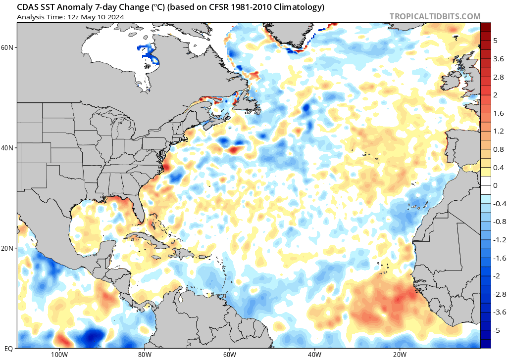
RAPID Array measuring North Atlantic SSTs.
For the last few years, observers have been speculating about when the North Atlantic will start the next phase shift from warm to cold. Given the way 2018 went and 2019 is following, this may be the onset. First some background.

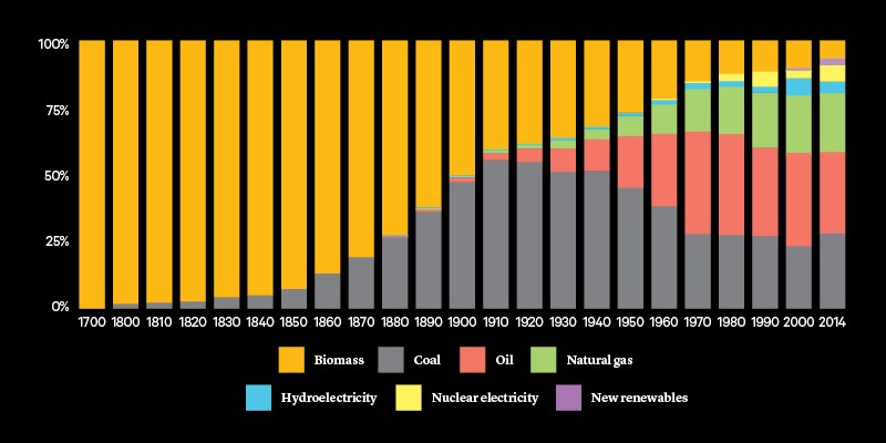
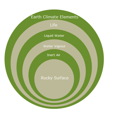
. Source: Energy and Education Canada
An example is this report in May 2015 The Atlantic is entering a cool phase that will change the world’s weather by Gerald McCarthy and Evan Haigh of the RAPID Atlantic monitoring project. Excerpts in italics with my bolds.
This is known as the Atlantic Multidecadal Oscillation (AMO), and the transition between its positive and negative phases can be very rapid. For example, Atlantic temperatures declined by 0.1ºC per decade from the 1940s to the 1970s. By comparison, global surface warming is estimated at 0.5ºC per century – a rate twice as slow.
In many parts of the world, the AMO has been linked with decade-long temperature and rainfall trends. Certainly – and perhaps obviously – the mean temperature of islands downwind of the Atlantic such as Britain and Ireland show almost exactly the same temperature fluctuations as the AMO.
Atlantic oscillations are associated with the frequency of hurricanes and droughts. When the AMO is in the warm phase, there are more hurricanes in the Atlantic and droughts in the US Midwest tend to be more frequent and prolonged. In the Pacific Northwest, a positive AMO leads to more rainfall.
A negative AMO (cooler ocean) is associated with reduced rainfall in the vulnerable Sahel region of Africa. The prolonged negative AMO was associated with the infamous Ethiopian famine in the mid-1980s. In the UK it tends to mean reduced summer rainfall – the mythical “barbeque summer”.Our results show that ocean circulation responds to the first mode of Atlantic atmospheric forcing, the North Atlantic Oscillation, through circulation changes between the subtropical and subpolar gyres – the intergyre region. This a major influence on the wind patterns and the heat transferred between the atmosphere and ocean.
The observations that we do have of the Atlantic overturning circulation over the past ten years show that it is declining. As a result, we expect the AMO is moving to a negative (colder surface waters) phase. This is consistent with observations of temperature in the North Atlantic.
Cold “blobs” in North Atlantic have been reported, but they are usually winter phenomena. For example in April 2016, the sst anomalies looked like this

But by September, the picture changed to this

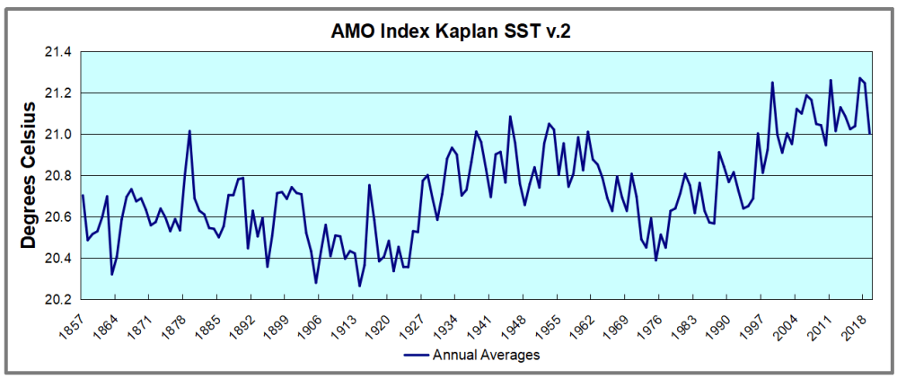
And we know from Kaplan AMO dataset, that 2016 summer SSTs were right up there with 1998 and 2010 as the highest recorded.
As the graph above suggests, this body of water is also important for tropical cyclones, since warmer water provides more energy. But those are annual averages, and I am interested in the summer pulses of warm water into the Arctic. As I have noted in my monthly HadSST3 reports, most summers since 2003 there have been warm pulses in the north atlantic.
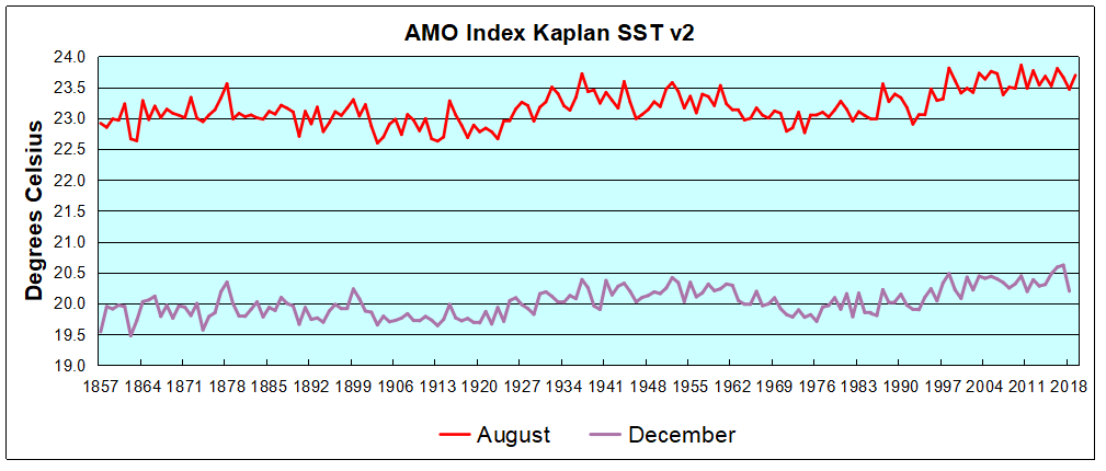
The AMO Index is from from Kaplan SST v2, the unaltered and not detrended dataset. By definition, the data are monthly average SSTs interpolated to a 5×5 grid over the North Atlantic basically 0 to 70N. The graph shows the warmest month August beginning to rise after 1993 up to 1998, with a series of matching years since. December 2016 set a record at 20.6C, but note the plunge down to 20.2C for December 2018, matching 2011 as the coldest years since 2000.
 November 2019 confirms the summer pulse weakening, along with 2018 well below other recent peak years since 1998. Because McCarthy refers to hints of cooling to come in the N. Atlantic, let’s take a closer look at some AMO years in the last 2 decades.
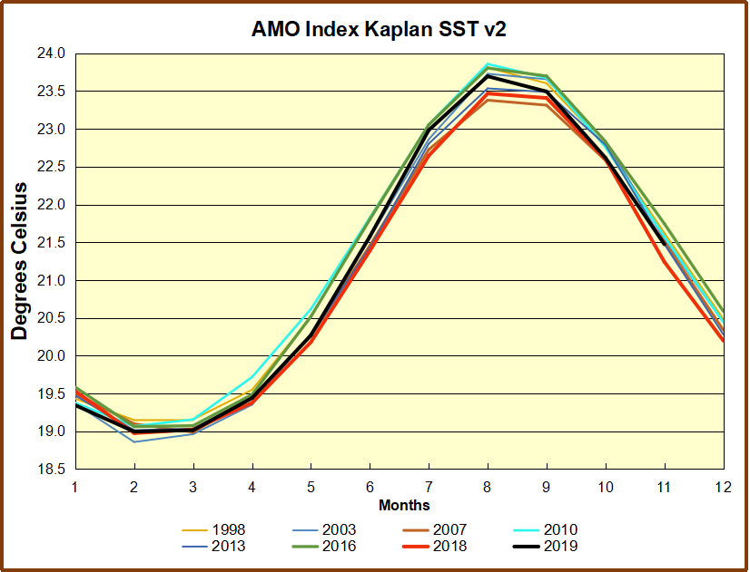 This graph shows monthly AMO temps for some important years. The Peak years were 1998, 2010 and 2016, with the latter emphasized as the most recent. The other years show lesser warming, with 2007 emphasized as the coolest in the last 20 years. Note the red 2018 line was at the bottom of all these tracks. The short black line shows that 2019 began slightly cooler than January 2018, then tracked closely before rising in the summer months, though still lower than the peak years. Now in November 2019 is again tracking warmer tthan 2018 but cooler than other recent years in the North Atlantic. For the 11 month annual average, 2019 is 0.1C higher than 2018, and both are more than 0.2C lower than the El Nino years of 2016 and 2017.
 Climate Litigation Watch is reporting the ruling by Judge Barry Ostrager ending the case brought by NYAG Leticia James against ExxonMobil. The loss could hardly be more complete. The full text of the ruling is here. The juicy bits are excerpted in italics below with my bolds.
Supreme Court of New York, New York County, the Honorable Barry Ostrager presiding.
Decision After Trial
Nothing in this opinion is intended to absolve ExxonMobil from responsibility for contributing to climate change through the emission of greenhouse gases in the production of its fossil fuel products. ExxonMobil does not dispute either that its operations produce greenhouse gases or that greenhouse gases contribute to climate change, But ExxonMobil is in the business of producing energy, and this is a securities fraud case, not a climate change case. Applying the applicable legal standards, the Court finds that the Office of the Attorney General failed to prove by a preponderance of the evidence that ExxonMobil made any material misrepresentations that “would have been viewed by a reasonable investor as having significantly altered the ‘total mix’ of information made available.” TSC Indusiries, Ine. v, Northway, Inc,, 426 U.S. 438 (1976).
The Office Attorney General is Not Entitled to Any Relief.
The Court also finds that the Office of the Attorney General is not entitled to any monetary damages or injunctive relief because the Office of the Attorney General did not prevail on its first and second causes of action. If the Court had reached the issues of damages, the Court would have found that the Office of the Attorney General failed to prove any damages by a preponderance of the evidence for the reasons stated infra.
The Office of the Attorney General had the burden to prove that ExxonMobil made misrepresentations and that ExxonMobil investors would have considered any alleged misrepresentations important in light of the “total mix of information” available to them. TSC Industries, Inc, v. Northway, Inc., 426 U.S. 438, 449 (1976). The Court finds there was no proof offered at trial that established material misrepresentations or omissions contained in any of ExxonMobil’s public disclosures that satisfy the applicable legal standard. The total mix of information available to ExxonMobil investors during the relevant period included an annual, publicly-filed report called the Outlook for Energy, the two March 2014 Reports, ExxonMobil’s Form 10-Ks, ExxonMobil’s annual Corporate Citizenship Reports, and a host of other publicly available information that was not the subject of testimony at trial (including ExxonMobil’s Annual Shareholder reports).
Significantly, there is no allegation in this case, and there was no proof adduced at trial, that anything ExxonMobil is alleged to have done or failed to have done affected ExxonMobil’s balance sheet, income statement, or any other financial disclosure. More importantly, the Office of the Attorney General’s case is largely focused on projections of proxy costs and GHG costs in 2030 and 2040. No reasonable investor during the period from 2013 to 2016 would make investment decisions based on speculative assumptions of costs that may be incurred 20+ or 30+ years in the future with respect to unidentified future projects. See Singh v. Cigna Corp., 918
At bottom, the case presented by the Office of the Attorney General is largely predicated upon the proposition, which this Court rejects, that during the period of time covered by the Complaint, ExxonMobil’s disclosures led the public to believe that its GHG cost assumptions for future projects had the same values assigned to its proxy cost of carbon. The existence of ExxonMobil’s DataGuide with separate sections and appendices for proxy costs and GHG costs is corroborative of ExxonMobil’s assertion that proxy cost of carbon and GHG costs are different metrics, a proposition of the Office of the Attorney General conceded before any testimony was presented at trial. Explicit statements in various publications confirmed this to be the case.
What the evidence at trial revealed is that ExxonMobil executives and employees were uniformly committed to rigorously discharging their duties in the most comprehensive and meticulous manner possible. More than half of the current and former ExxonMobil executives and employees who testified at trial have worked for ExxonMobil for the entirety of their careers. The testimony of these witnesses demonstrated that ExxonMobil has a culture of disciplined analysis, planning, accounting, and reporting.
To support its theory that the alleged misstatements in the March 31, 2014 publications were material, the Office of the Attorney General offered the expert testimony and expert report of Dr. Eli Bartov who concluded that there was inflation on the stock price of ExxonMobil from April 1, 2014 to June 1, 2017. Tr. 1149:25-1150:4. Dr. Bartov posited that the inflation period began after the alleged affirmative misrepresentations contained in the two March 31, 2014 publications. Significantly, the Office of the Attorney General offered no proof that there was any increase in the stock price of ExxonMobil immediately following the publication of Managing the Risk and Energy and Climate and Dr. Bartov perplexingly testified that he did not conduct an analysis of whether or not ExxonMobil’s stock increased as a result of the alleged misrepresentations in the March 31, 2014 publications “because it was completely unrelated to my analysis.” Tr. 1233:8-13. By contrast, ExxonMobil’s expert, Dr. Frank Allen Ferrell,” determined that there was no increase in ExxonMobil stock on April 1, 2014. Tr. 1967. In short, there is no evidence that any misleading statements in these publications inflated the price of ExxonMobil stock. See DX711 ¶ 15 Expert Report of Allen Ferrell.
None of Dr. Bartov’s corrective disclosures contain any statements from ExxonMobil acknowledging a misstatement or correcting a previous disclosure. Tr. 1208. They all pertain to regulatory investigations of ExxonMobil announced in the mainstream press. In short, the news of the California Attorney General’s reported investigation is precisely the kind of news that the Office of Attorney General’s witness Rodger Reed characterized as “headline risk.” Additionally, as ExxonMobil’s highly credentialed expert, Dr. Ferrell, testified, there is something circular about claiming that a stock drop precipitated by the announcement of an investigation constitutes evidence of wrongdoing. Indeed, by Dr. Bartov’s reasoning, any decline in the value of ExxonMobil stock after the June 2, 2017 filing of the Office of the Attorney General’s complaint is the result of an ill-conceived initiative of the Office of the Attorney General.
V. Conclusion
In sum, the Office of the Attorney General failed to prove, by a preponderance of the evidence, that ExxonMobil made any material misstatements or omissions about its practices and procedures that misled any reasonable investor. The Office of the Attorney General produced no testimony either from any investor who claimed to have been misled by any disclosure, even though the Office of the Attorney General had previously represented it would call such individuals as trial witnesses. ExxonMobil disclosed its use of both the proxy cost and the GHG metrics no later than 2014. Perhaps, the 2014 paragraph in Managing the Risks which indicated that ExxonMobil applied a GHG cost “where appropriate” and which was the subject of questioning of virtually every witness in the case could have been written in bold type, but the sentence was consistent with other ExxonMobil disclosures and ExxonMobil’s business practices. The publication of Managing the Risks had no market impact and was, as far as the evidence adduced at trial reflected, essentially ignored by the investment community.
The testimony of all the present and former ExxonMobil employees who were called either as adverse witnesses by the Office of the Attorney General or as defense witnesses by ExxonMobil was uniformly favorable to ExxonMobil, and the Court credited the testimony of each of those witnesses. The testimony of the expert witnesses called by the Office of the Attorney General was eviscerated on cross-examination and by ExxonMobil’s expert witnesses. Confronted with the disclosures in ExxonMobil’s Corporate Citizenship Reports, Form 10-K’s, and ExxonMobil’s annually published Outlook, the Office of the Attorney General failed to prove by a preponderance of the evidence that any alleged misrepresentation in Managing the Risks and Energy and Climate (or any other disclosure by ExxonMobil) was false and material in the context of the total mix of information available to the public.
For all of these reasons, the claims asserted by the Office of the Attorney General under the Martin Act and Executive Law § 63(12) are denied, and the action is dismissed with prejudice.
Dated: December 10, 2019
Barry R. Ostrager, JSC
Background: New York AG’s Disgraceful Exxon Trial
A recent study exposes the lack of relation between CO2 and hurricanes in the US North Atlantic. Ryan Truchelut and Erica Staehling published An Energetic Perspective on United States Tropical Cyclone Landfall Droughts in Geophysical Research Letters, December 2017. Excerpts in italics with my bolds. H/T Craig Idso and Master Resource
Summary
The 2017 Atlantic hurricane season has been extremely active both in terms of the strength of the tropical cyclones that have developed and the amount of storm activity that has occurred near the United States. This is even more notable as it comes at the end of an extended period of below normal U.S. hurricane activity, as no major (category 3 or higher) hurricanes made landfall from 2006 through 2016. Our study examines how rare the recent “landfall drought” actually was using a record of the estimated total energy of storms over the U.S., rather than prior methods of counting hurricanes making U.S. landfall. Using this technique, we found that 2006–2015 was in the least active 10% of 10 year periods in terms of U.S. tropical cyclone energy but that several less active periods had occurred in the last 50 years. The 2006–2016 drought years did record the lowest percentage of storm activity occurring over the U.S. relative to what was observed over the entire Atlantic. This finding is further evidence for a trade‐off between atmospheric conditions favoring hurricane development and those that are most favorable for powerful storms to move towards the U.S. coastline.
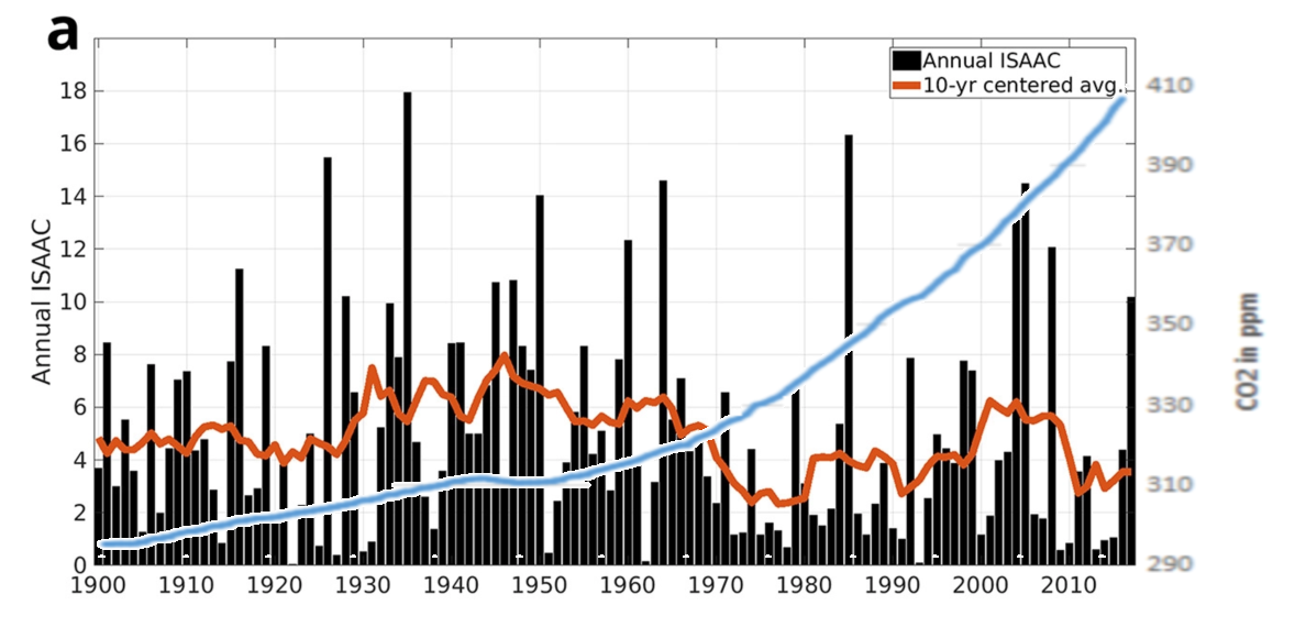
[The graph above shows exhibit 2a from Truchelut and Staehling overlaid with the record of atmospheric CO2 concentrations. From NOAA combining Mauna Loa with earlier datasets.]
To determine Integrated Storm Activity Annually over the Continental U.S. (ISAAC) from 1900 through 2017, we summed this landfall ACE spatially over the entire continental U.S. and temporally over each hour of each hurricane season. We used the same methodology to calculate integrated annual landfall ACE for five additional geographic subsets of the continental U.S.

Figure 2 (a) Time series of ISAAC for 1900–2017, with a 10 year centered average value (red). (b) Spatial distribution of ACE over the U.S. for 1900–2017, summing all hourly intensities of TCs occurring within 0.5° of each grid point.
ISAAC accounts for 4.3% of annual total Atlantic ACE since 1950, with a seasonal median value of 3.4%. The maximum value of 18.5% occurred in 1985, in which there were six U.S. hurricane landfalls despite near‐normal basin‐wide total ACE. Minimum values of lower than 0.5% occurred in several years in the time series. In 2017, around 4.5% of total Atlantic TC activity occurred over the continental U.S., almost exactly in‐line with the long‐term mean percentage.
Ultimately, the 2017 hurricane season is a stark reminder that understanding interannual variability in TC hazard risk is of utmost importance to scientists, policymakers, emergency managers, insurers, and coastal citizens. The use of energetic metrics is a step toward better acuity in diagnostic and predictive modeling of this risk variance; for instance, in years during which three hurricanes made U.S. landfall, the number of ACE units over the continental U.S. ranged from fewer than 4 to more than 14. As a means of more fully incorporating the reliable climatological record into this and future studies, landfall ACE is promising for properly contextualizing the rarity of events like the recent landfall drought.
Wrap Up 2019 Hurricane Season (Previous post)

Figure: Global Hurricane Frequency (all & major) — 12-month running sums. The top time series is the number of global tropical cyclones that reached at least hurricane-force (maximum lifetime wind speed exceeds 64-knots). The bottom time series is the number of global tropical cyclones that reached major hurricane strength (96-knots+). Adapted from Maue (2011) GRL.
This post refers to statistics for this year’s Atlantic and Global Hurricane season, now likely completed. The chart above was updated by Ryan Maue yesterday. A detailed report is provided by the Colorado State University Tropical Meteorology Project, directed by Dr. William Gray until his death in 2016. More from Bill Gray in a reprinted post at the end.
The article is Summary of 2019 Atlantic Tropical Cyclone Activity and Verification of Authors’ Seasonal And Two-week Forecasts. By Philip J. Klotzbach, Michael M. Bell, and Jhordanne Jones In Memory of William M. Gray. Excerpts in italics with my bolds.
Summary:
The 2019 Atlantic hurricane season was slightly above average and had a little more activity than what was predicted by our June-August updates. The climatological peak months of the hurricane season were characterized by a below-average August, a very active September, and above-average named storm activity but below-average hurricane activity in October. Hurricane Dorian was the most impactful hurricane of 2019, devastating the northwestern Bahamas before bringing significant impacts to the
southeastern United States and the Atlantic Provinces of Canada. Tropical Storm Imelda also brought significant flooding to southeast Texas.
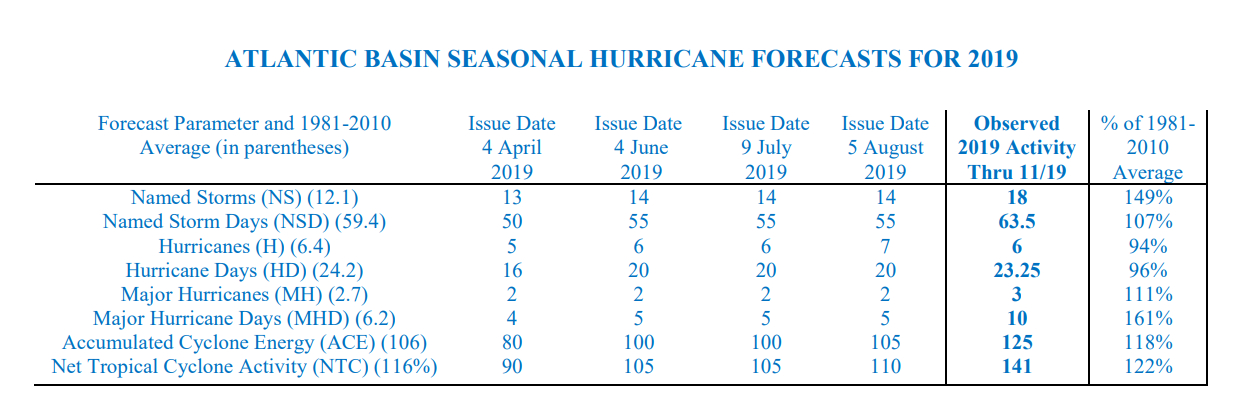
Open image in new tab to enlarge.
The 2019 hurricane season overall was slightly above average. The season was characterized by an above-average number of named storms and a near-average number of hurricanes and major hurricanes. Our initial seasonal forecast issued in April somewhat underestimated activity, while seasonal updates issued in June, July and August, respectively, slightly underestimated overall activity. The primary reason for the underestimate was due to a more rapid abatement of weak El Niño conditions than was originally anticipated. August was a relatively quiet month for Atlantic TC activity, while September was well above-average. While October had an above-average number of named storm formations, overall Accumulated Cyclone Energy was slightly below normal.

Figure: Last 4-decades of Global and Northern Hemisphere Accumulated Cyclone Energy: 24 month running sums. Note that the year indicated represents the value of ACE through the previous 24-months for the Northern Hemisphere (bottom line/gray boxes) and the entire global (top line/blue boxes). The area in between represents the Southern Hemisphere total ACE.
Previous Post: Bill Gray: H20 is Climate Control Knob, not CO2

William Mason Gray (1929-2016), pioneering hurricane scientist and forecaster and professor of atmospheric science at Colorado State University.
Dr. William Gray made a compelling case for H2O as the climate thermostat, prior to his death in 2016. Thanks to GWPF for publishing posthumously Bill Gray’s understanding of global warming/climate change. The paper was compiled at his request, completed and now available as Flaws in applying greenhouse warming to Climate Variability This post provides some excerpts in italics with my bolds and some headers. Readers will learn much from the entire document (title above is link to pdf).
The Fundamental Correction
The critical argument that is made by many in the global climate modeling (GCM) community is that an increase in CO2 warming leads to an increase in atmospheric water vapor, resulting in more warming from the absorption of outgoing infrared radiation (IR) by the water vapor. Water vapor is the most potent greenhouse gas present in the atmosphere in large quantities. Its variability (i.e. global cloudiness) is not handled adequately in GCMs in my view. In contrast to the positive feedback between CO2 and water vapor predicted by the GCMs, it is my hypothesis that there is a negative feedback between CO2 warming and and water vapor. CO2 warming ultimately results in less water vapor (not more) in the upper troposphere. The GCMs therefore predict unrealistic warming of global temperature. I hypothesize that the Earth’s energy balance is regulated by precipitation (primarily via deep cumulonimbus (Cb) convection) and that this precipitation counteracts warming due to CO2.
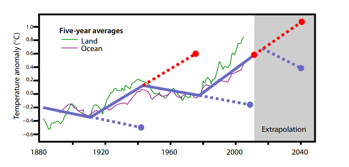
Figure 14: Global surface temperature change since 1880. The dotted blue and dotted red lines illustrate how much error one would have made by extrapolating a multi-decadal cooling or warming trend beyond a typical 25-35 year period. Note the recent 1975-2000 warming trend has not continued, and the global temperature remained relatively constant until 2014.
Projected Climate Changes from Rising CO2 Not Observed
Continuous measurements of atmospheric CO2, which were first made at Mauna Loa, Hawaii in 1958, show that atmospheric concentrations of CO2 have risen since that time. The warming influence of CO2 increases with the natural logarithm (ln) of the atmosphere’s CO2 concentration. With CO2 concentrations now exceeding 400 parts per million by volume (ppm), the Earth’s atmosphere is slightly more than halfway to containing double the 280 ppm CO2 amounts in 1860 (at the beginning of the Industrial Revolution).∗
We have not observed the global climate change we would have expected to take place, given this increase in CO2. Assuming that there has been at least an average of 1 W/m2 CO2 blockage of IR energy to space over the last 50 years and that this energy imbalance has been allowed to independently accumulate and cause climate change over this period with no compensating response, it would have had the potential to bring about changes in any one of the following global conditions:
Earth Climate System Compensates for CO2
If CO2 gain is the only influence on climate variability, large and important counterbalancing influences must have occurred over the last 50 years in order to negate most of the climate change expected from CO2’s energy addition. Similarly, this hypothesized CO2-induced energy gain of 1 W/m2 over 50 years must have stimulated a compensating response that acted to largely negate energy gains from the increase in CO2.
The continuous balancing of global average in-and-out net radiation flux is therefore much larger than the radiation flux from anthropogenic CO2. For example, 342 W/m2, the total energy budget, is almost 100 times larger than the amount of radiation blockage expected from a CO2 doubling over 150 years. If all other factors are held constant, a doubling of CO2 requires a warming of the globe of about 1◦C to enhance outward IR flux by 3.7 W/m2 and thus balance the blockage of IR flux to space.
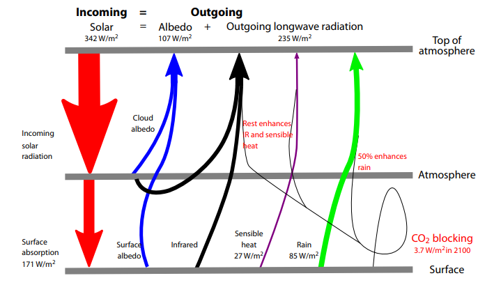
Figure 2: Vertical cross-section of the annual global energy budget. Determined from a combination of satellite-derived radiation measurements and reanalysis data over the period of 1984–2004.
This pure IR energy blocking by CO2 versus compensating temperature increase for radiation equilibrium is unrealistic for the long-term and slow CO2 increases that are occurring. Only half of the blockage of 3.7 W/m2 at the surface should be expected to go into an temperature increase. The other half (about 1.85 W/m2) of the blocked IR energy to space will be compensated by surface energy loss to support enhanced evaporation. This occurs in a similar way to how the Earth’s surface energy budget compensates for half its solar gain of 171 W/m2 by surface-to-air upward water vapor flux due to evaporation.
Assuming that the imposed extra CO2 doubling IR blockage of 3.7 W/m2 is taken up and balanced by the Earth’s surface in the same way as the solar absorption is taken up and balanced, we should expect a direct warming of only ~0.5◦C for a doubling of CO2. The 1◦C expected warming that is commonly accepted incorrectly assumes that all the absorbed IR goes to the balancing outward radiation with no energy going to evaporation.
Consensus Science Exaggerates Humidity and Temperature Effects
A major premise of the GCMs has been their application of the National Academy of Science (NAS) 1979 study3 – often referred to as the Charney Report – which hypothesized that a doubling of atmospheric CO2 would bring about a general warming of the globe’s mean temperature of 1.5–4.5◦C (or an average of ~3.0◦C). These large warming values were based on the report’s assumption that the relative humidity (RH) of the atmosphere remains quasiconstant as the globe’s temperature increases. This assumption was made without any type of cumulus convective cloud model and was based solely on the Clausius–Clapeyron (CC) equation and the assumption that the RH of the air will remain constant during any future CO2-induced temperature changes. If RH remains constant as atmospheric temperature increases, then the water vapor content in the atmosphere must rise exponentially.
With constant RH, the water vapor content of the atmosphere rises by about 50% if atmospheric temperature is increased by 5◦C. Upper tropospheric water vapor increases act to raise the atmosphere’s radiation emission level to a higher and thus colder level. This reduces the amount of outgoing IR energy which can escape to space by decreasing T^4.
These model predictions of large upper-level tropospheric moisture increases have persisted in the current generation of GCM forecasts.§ These models significantly overestimate globally-averaged tropospheric and lower stratospheric (0–50,000 feet) temperature trends since 1979 (Figure 7).
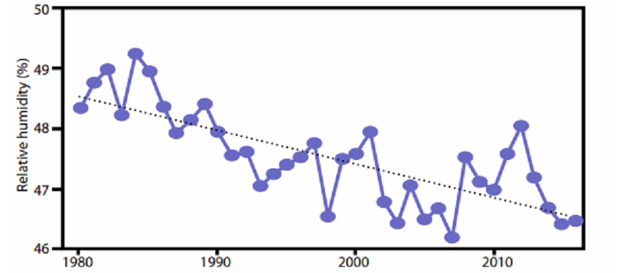
Figure 8: Decline in upper tropospheric RH. Annually-averaged 300 mb relative humidity for the tropics (30°S–30°N). From NASA-MERRA2 reanalysis for 1980–2016. Black dotted line is linear trend.
All of these early GCM simulations were destined to give unrealistically large upper-tropospheric water vapor increases for doubling of CO2 blockage of IR energy to space, and as a result large and unrealistic upper tropospheric temperature increases were predicted. In fact, if data from NASA-MERRA24 and NCEP/NCAR5 can be believed, upper tropospheric RH has actually been declining since 1980 as shown in Figure 8. The top part of Table 1 shows temperature and humidity differences between very wet and dry years in the tropics since 1948; in the wettest years, precipitation was 3.9% higher than in the driest ones. Clearly, when it rains more in the tropics, relative and specific humidity decrease. A similar decrease is seen when differencing 1995–2004 from 1985–1994, periods for which the equivalent precipitation difference is 2%. Such a decrease in RH would lead to a decrease in the height of the radiation emission level and an increase in IR to space.
The Earth’s natural thermostat – evaporation and precipitation
What has prevented this extra CO2-induced energy input of the last 50 years from being realized in more climate warming than has actually occurred? Why was there recently a pause in global warming, lasting for about 15 years? The compensating influence that prevents the predicted CO2-induced warming is enhanced global surface evaporation and increased precipitation.
Annual average global evaporational cooling is about 80 W/m2 or about 2.8 mm per day. A little more than 1% extra global average evaporation per year would amount to 1.3 cm per year or 65 cm of extra evaporation integrated over the last 50 years. This is the only way that such a CO2-induced , 1 W/m2 IR energy gain sustained over 50 years could occur without a significant alteration of globally-averaged surface temperature. This hypothesized increase in global surface evaporation as a response to CO2-forced energy gain should not be considered unusual. All geophysical systems attempt to adapt to imposed energy forcings by developing responses that counter the imposed action. In analysing the Earth’s radiation budget, it is incorrect to simply add or subtract energy sources or sinks to the global system and expect the resulting global temperatures to proportionally change. This is because the majority of CO2-induced energy gains will not go into warming the atmosphere. Various amounts of CO2-forced energy will go into ocean surface storage or into ocean energy gain for increased surface evaporation. Therefore a significant part of the CO2 buildup (~75%) will bring about the phase change of surface liquid water to atmospheric water vapour. The energy for this phase change must come from the surface water, with an expenditure of around 580 calories of energy for every gram of liquid that is converted into vapour. The surface water must thus undergo a cooling to accomplish this phase change.
Therefore, increases in anthropogenic CO2 have brought about a small (about 0.8%) speeding up of the globe’s hydrologic cycle, leading to more precipitation, and to relatively little global temperature increase. Therefore, greenhouse gases are indeed playing an important role in altering the globe’s climate, but they are doing so primarily by increasing the speed of the hydrologic cycle as opposed to increasing global temperature.
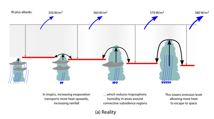
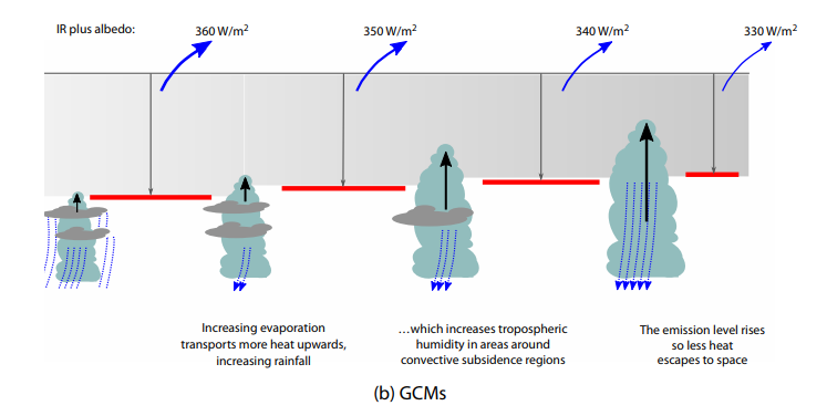 Figure 9: Two contrasting views of the effects of how the continuous intensification of deep
cumulus convection would act to alter radiation flux to space.
The top (bottom) diagram represents a net increase (decrease) in radiation to space
Tropical Clouds Energy Control Mechanism
It is my hypothesis that the increase in global precipitation primarily arises from an increase in deep tropical cumulonimbus (Cb) convection. The typical enhancement of rainfall and updraft motion in these areas together act to increase the return flow mass subsidence in the surrounding broader clear and partly cloudy regions. The upper diagram in Figure 9 illustrates the increasing extra mass flow return subsidence associated with increasing depth and intensity of cumulus convection. Rainfall increases typically cause an overall reduction of specific humidity (q) and relative humidity (RH) in the upper tropospheric levels of the broader scale surrounding convective subsidence regions. This leads to a net enhancement of radiation flux to space due to a lowering of the upper-level emission level. This viewpoint contrasts with the position in GCMs, which suggest that an increase in deep convection will increase upper-level water vapour.
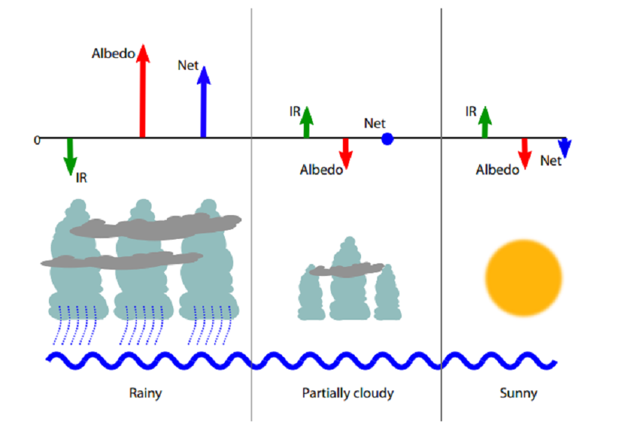
Figure 10: Conceptual model of typical variations of IR, albedo and net (IR + albedo) associated with three different areas of rain and cloud for periods of increased precipitation.
The albedo enhancement over the cloud–rain areas tends to increase the net (IR + albedo) radiation energy to space more than the weak suppression of (IR + albedo) in the clear areas. Near-neutral conditions prevail in the partly cloudy areas. The bottom diagram of Figure 9 illustrates how, in GCMs, Cb convection erroneously increases upper tropospheric moisture. Based on reanalysis data (Table 1, Figure 8) this is not observed in the real atmosphere.
Ocean Overturning Circulation Drives Warming Last Century
A slowing down of the global ocean’s MOC is the likely cause of most of the global warming that has been observed since the latter part of the 19th century.15 I hypothesize that shorter multi-decadal changes in the MOC16 are responsible for the more recent global warming periods between 1910–1940 and 1975–1998 and the global warming hiatus periods between 1945–1975 and 2000–2013.
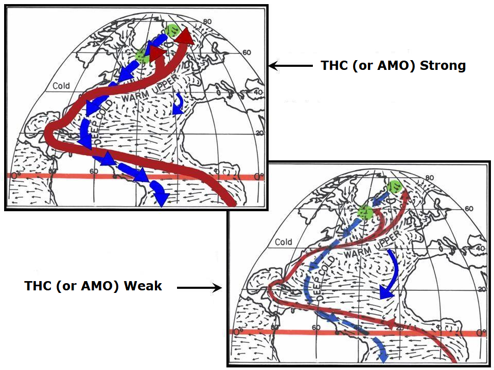
Figure 12: The effect of strong and weak Atlantic THC. Idealized portrayal of the primary Atlantic Ocean upper ocean currents during strong and weak phases of the thermohaline circulation (THC)
Figure 13 shows the circulation features that typically accompany periods when the MOC is stronger than normal and when it is weaker than normal. In general, a strong MOC is associated with a warmer-than-normal North Atlantic, increased Atlantic hurricane activity, increased blocking action in both the North Atlantic and North Pacific and weaker westerlies in the mid-latitude Southern Hemisphere. There is more upwelling of cold water in the South Pacific and Indian Oceans, and an increase in global rainfall of a few percent occurs. This causes the global surface temperatures to cool. The opposite occurs when the MOC is weaker than normal.
The average strength of the MOC over the last 150 years has likely been below the multimillennium average, and that is the primary reason we have seen this long-term global warming since the late 19th century. The globe appears to be rebounding from the conditions of the Little Ice Age to conditions that were typical of the earlier ‘Medieval’ and ‘Roman’ warm periods.
Summary and Conclusions
The Earth is covered with 71% liquid water. Over the ocean surface, sub-saturated winds blow, forcing continuous surface evaporation. Observations and energy budget analyses indicate that the surface of the globe is losing about 80 W/m2 of energy from the global surface evaporation process. This evaporation energy loss is needed as part of the process of balancing the surface’s absorption of large amounts of incoming solar energy. Variations in the strength of the globe’s hydrologic cycle are the way that the global climate is regulated. The stronger the hydrologic cycle, the more surface evaporation cooling occurs, and greater the globe’s IR flux to space. The globe’s surface cools when the hydrologic cycle is stronger than average and warms when the hydrologic cycle is weaker than normal. The strength of the hydrologic cycle is thus the primary regulator of the globe’s surface temperature. Variations in global precipitation are linked to long-term changes in the MOC (or THC).
I have proposed that any additional warming from an increase in CO2 added to the atmosphere is offset by an increase in surface evaporation and increased precipitation (an increase in the water cycle). My prediction seems to be supported by evidence of upper tropospheric drying since 1979 and the increase in global precipitation seen in reanalysis data. I have shown that the additional heating that may be caused by an increase in CO2 results in a drying, not a moistening, of the upper troposphere, resulting in an increase of outgoing radiation to space, not a decrease as proposed by the most recent application of the greenhouse theory.
Deficiencies in the ability of GCMs to adequately represent variations in global cloudiness, the water cycle, the carbon cycle, long-term changes in deep-ocean circulation, and other important mechanisms that control the climate reduce our confidence in the ability of these models to adequately forecast future global temperatures. It seems that the models do not correctly handle what happens to the added energy from CO2 IR blocking.
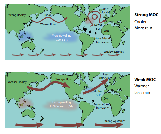
Figure 13: Effect of changes in MOC: top, strong MOC; bottom weak MOC. SLP: sea level pressure; SST, sea surface temperature.
Solar variations, sunspots, volcanic eruptions and cosmic ray changes are energy-wise too small to play a significant role in the large energy changes that occur during important multi-decadal and multi-century temperature changes. It is the Earth’s internal fluctuations that are the most important cause of climate and temperature change. These internal fluctuations are driven primarily by deep multi-decadal and multi-century ocean circulation changes, of which naturally varying upper-ocean salinity content is hypothesized to be the primary driving mechanism. Salinity controls ocean density at cold temperatures and at high latitudes where the potential deep-water formation sites of the THC and SAS are located. North Atlantic upper ocean salinity changes are brought about by both multi-decadal and multi-century induced North Atlantic salinity variability.
Footnote:
The main point from Bill Gray was nicely summarized in a previous post Earth Climate Layers
The most fundamental of the many fatal mathematical flaws in the IPCC related modelling of atmospheric energy dynamics is to start with the impact of CO2 and assume water vapour as a dependent ‘forcing’. This has the tail trying to wag the dog. The impact of CO2 should be treated as a perturbation of the water cycle. When this is done, its effect is negligible. — Dr. Dai Davies
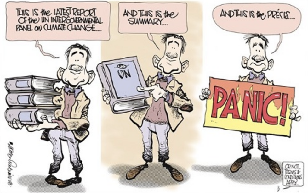
Deutsche Welle provides this opinion article during the second week of COP25: In times of climate change, panic rules. Excerpts in italics with my bolds
As the planet heats up, so does the debate about climate change. Sensible debate is becoming increasingly difficult in these fearful times, and Zoran Arbutina says people with rational arguments are at a disadvantage.
“I want you to panic. I want you to feel the fear I feel every day. … I want you to act as if our house is on fire.” The words spoken by teenage climate activist Greta Thunberg at the World Economic Forum in Davos in January are certain to end up high on the list of the year’s most important quotes.
It’s rare to see someone express the zeitgeist so clearly. It’s as if millions of mainly young people were just waiting for someone to give them the go-ahead to finally do what they needed to do: stand up, take to the streets and speak out against man-made climate change.

In Germany, even more so than in other European countries, it seems the urgent call of the young Swedish activist has unleashed a veritable avalanche of protest and outrage, overrunning everything in its path. These days, panic rules the country — and it’s putting pressure on politicians.
Just do ‘something’
More and more German cities have declared a “climate emergency,” with even the European Parliament recently getting carried away and following suit. Such declarations are essentially symbolic; the climate isn’t any better off as a result, but that’s not the point. It’s all about creating a social climate of fear, of panic.
The latest alarming contribution is a new report by environmental think tank Germanwatch, which ranked Germany as the third-most weather-affected country in the world in 2018, after Japan and the Philippines. Germanwatch said its Global Climate Risk Index, published annually, doesn’t allow for conclusions to be drawn about how climate change has influenced extreme weather events, and said its analysis included “statistical uncertainties.” But that’s not important —what matters is the warning that rising temperatures will make extreme weather occurrences more likely. It wasn’t much, but the report was enough to spread fear even further.
Fear, however, usually isn’t the best guide. When people panic, they rarely make good decisions — and that’s certainly the case for a society. In a democracy, political decisions should be based on rational arguments and reason. In a climate of fear, rational arguments only come out when they help to further the agenda.

Signs of climate change?
An example: those who question global warming during extreme cold spells (yes, they still happen!) are often informed that there is a difference between climate and weather. If, on the other hand, we go through two dry, hot summers in a row, it’s almost always seen as a sign of runaway climate change.
Activists like to point to allegedly unambiguous scientific findings to make their claims that climate change is upon us. But when a renowned climate researcher like Hans von Storch says that protesters only “mix up” and “exaggerate” everything, his scientific integrity is immediately called into question.
Exaggerated expectations
While climate activists have pressured Germany’s traditional political parties, the Greens have sailed on the waves of the environmental movement and made huge gains in recent elections. But a new conflict awaits on the horizon: should the environmentalists return to power on the federal level, the Greens and their voters will find that they cannot fulfill the raised expectations of their followers. That failure will trigger fresh disappointment, anger and even more fear.
Of course, one can and should argue about climate policy. And naturally, the climate activists have made some good points. But climate policy must be decided as everything else in politics: through societal debate, and the belief in the power of the better argument. Climate change is too important an issue to be left to climate activists alone. Their worries should be taken seriously, as should the worries of many other social groups. But being dominated by the fears of a single group is never a good approach.

Previous Post Shows How Panic Distorts Reality (from last summer)
People who struggle with anxiety are known to have moments of “hair on fire.” IOW, letting your fears take over is like setting your own hair on fire. Currently the media, pandering as always to primal fear instincts, is declaring that the Arctic is on fire, and it is our fault. Let’s see what we can do to help them get a grip.
1. Summer is fire season for northern boreal forests and tundra.
From the Canadian National Forestry Database
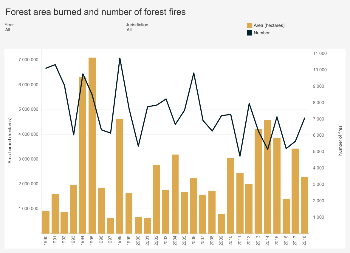
Since 1990, “wildland fires” across Canada have consumed an average of 2.5 million hectares a year.
| Recent Canadian Forest Fire Activity | 2015 | 2016 | 2017 |
| Area burned (hectares) | 3,861,647 | 1,416,053 | 3,371,833 |
| Number of fires | 7,140 | 5,203 | 5,611 |
The total area of Forest and other wooded land in Canada is 396,433,600 (hectares). So the data says that every average year 0.6% of Canadian wooded area burns due to numerous fires, ranging from 1000 in a slow year to over 10,000 fires and 7M hectares burned in 1995.
2. With the warming since 1980 some years have seen increased areas burning.
From Wildland Fire in High Latitudes, A. York et al. (2017)
Despite the low annual temperatures and short growing seasons characteristic of northern ecosystems, wildland fire affects both boreal forest (the broad band of mostly coniferous trees that generally stretches across the area north of the July 13° C isotherm in North America and Eurasia, also known as Taiga) and adjacent tundra regions. In fact, fire is the dominant ecological disturbance in boreal forest, the world’s largest terrestrial biome. Fire disturbance affects these high latitude systems at multiple scales, including direct release of carbon through combustion (Kasischke et al., 2000) and interactions with vegetation succession (Mann et al., 2012; Johnstone et al., 2010), biogeochemical cycles (Bond-Lamberty et al., 2007), energy balance (Rogers et al., 2015), and hydrology (Liu et al., 2005). About 35% of global soil carbon is stored in tundra and boreal systems (Scharlemann et al., 2014) that are potentially vulnerable to fire disturbance (Turetsky et al., 2015). This brief report summarizes evidence from Alaska and Canada on variability and trends in fire disturbance in high latitudes and outlines how short-term fire weather conditions in these regions influence area burned.
Climate is a dominant control of fire activity in both boreal and tundra ecosystems. The relationship between climate and fire is strongly nonlinear, with the likelihood of fire occurrence within a 30-year period much higher where mean July temperatures exceed 13.4° C (56° F) (Young et al., 2017). High latitude fire regimes appear to be responding rapidly to recent environmental changes associated with the warming climate. Although highly variable, area burned has increased over the past several decades in much of boreal North America (Kasischke and Turetsky, 2006; Gillett et al., 2004). Since the early 1960s, the number of individual fire events and the size of those events has increased, contributing to more frequent large fire years in northwestern North America (Kasischke and Turetsky, 2006). Figure 1 shows annual area burned per year in Alaska (a) and Northwest Territories (b) since 1980, including both boreal and tundra regions.

[Comment: Note that both Alaska and NW Territories see about 500k hectares burned on average each year since 1980. And in each region, three years have been much above that average, with no particular pattern as to timing.]
Recent large fire seasons in high latitudes include 2014 in the Northwest Territories, where 385 fires burned 8.4 million acres, and 2015 in Alaska, where 766 fires burned 5.1 million acres (Figs. 1 & 2)—more than half the total acreage burned in the US (NWT, 2015; AICC, 2015). Multiple northern communities have been threatened or damaged by recent wildfires, notably Fort McMurray, Alberta, where 88,000 people were evacuated and 2400 structures were destroyed in May 2016. Examples of recent significant tundra fires include the 2007 Anaktuvuk River Fire, the largest and longest-burning fire known to have occurred on the North Slope of Alaska (256,000 acres), which initiated widespread thermokarst development (Jones et al., 2015). An unusually large tundra fire in western Greenland in 2017 received considerable media attention.
Large fire events such as these require the confluence of receptive fuels that will promote fire growth once ignited, periods of warm and dry weather conditions, and a source of ignition—most commonly, convective thunderstorms that produce lightning ignitions. High latitude ecosystems are characterized by unique fuels—in particular, fast-drying beds of mosses, lichens, resinous shrubs, and accumulated organic material (duff) that underlie dense, highly flammable conifers. These understory fuels cure rapidly during warm, dry periods with long daylight hours in June and July. Consequently, extended periods of drought are not required to increase fire danger to extreme levels in these systems.
Most acreage burned in high latitude systems occurs during sporadic periods of high fire activity; 50% of the acreage burned in Alaska from 2002 to 2010 was consumed in just 36 days (Barrett et al., 2016). Figure 3 shows cumulative acres burned in the four largest fire seasons in Alaska since 1990 (from Fig. 1) and illustrates the varying trajectories of each season. Some seasons show periods of rapid growth during unusually warm and dry weather (2004, 2009, 2015), while others (2004 and 2005) were prolonged into the fall in the absence of season-ending rain events. In 2004, which was Alaska’s largest wildfire season at 6.6 million acres, the trajectory was characterized by both rapid mid-season growth and extended activity into September. These different pathways to large fire seasons demonstrate the importance of intraseasonal weather variability and the timing of dynamical features. As another example, although not large in total acres burned, the 2016 wildland fire season in Alaska was more than 6 months long, with incidents requiring response from mid-April through late October (AICC, 2016).
3. Wildfires are part of the ecology cycle making the biosphere sustainable.
Forest Fire Ecology: Fire in Canada’s forests varies in its role and importance.
In the moist forests of the west coast, wildland fires are relatively infrequent and generally play a minor ecological role.
In boreal forests, the complete opposite is true. Fires are frequent and their ecological influence at all levels—species, stand and landscape—drives boreal forest vegetation dynamics. This in turn affects the movement of wildlife populations, whose need for food and cover means they must relocate as the forest patterns change.
lThe Canadian boreal forest is a mosaic of species and stands. It ranges in composition from pure deciduous and mixed deciduous-coniferous to pure coniferous stands.
The diversity of the forest mosaic is largely the result of many fires occurring on the landscape over a long period of time. These fires have varied in frequency, intensity, severity, size, shape and season of burn.
The fire management balancing act: Fire is a vital ecological component of Canadian forests and will always be present.
Not all wildland fires should (or can) be controlled. Forest agencies work to harness the force of natural fire to take advantage of its ecological benefits while at the same time limiting its potential damage and costs.
Tundra Fire Ecology
From Arctic tundra fires: natural variability and responses to climate change, Feng Sheng Hu et al. (2015)
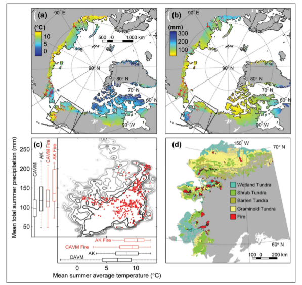
Circumpolar tundra fires have primarily occurred in the portions of the Arctic with warmer summer conditions, especially Alaska and northeastern Siberia (Figure 1). Satellite-based estimates (Giglio et al. 2010; Global Fire Emissions Database 2015) show that for the period of 2002–2013, 0.48% of the Alaskan tundra has burned, which is four times the estimate for the Arctic as a whole (0.12%; Figure 1). These estimates encompass tundra ecoregions with a wide range of fire regimes. For instance, within Alaska, the observational record of the past 60 years indicates that only 1.4% of the North Slope ecoregion has burned (Rocha et al. 2012); 68% of the total burned area in this ecoregion was associated with a single event, the 2007 AR Fire.
The Noatak and Seward Peninsula ecoregions are the most flammable of the tundra biome, and both contain areas that have experienced multiple fires within the past 60 years (Rocha et al. 2012). This high level of fire activity suggests that fuel availability has not been a major limiting factor for fire occurrence in some tundra regions, probably because of the rapid post-fire recovery of tundra vegetation (Racine et al. 1987; Bret-Harte et al. 2013) and the abundance of peaty soils.
However, the wide range of tundra-fire regimes in the modern record results from spatial variations in climate and fuel conditions among ecoregions. For example, frequent tundra burning in the Noatak ecoregion reflects relatively warm/dry climate conditions, whereas the extreme rarity of tundra fires in southwestern Alaska reflects a wet regional climate and abundant lakes that act as natural firebreaks.
Fire alters the surface properties, energy balance, and carbon (C) storage of many terrestrial ecosystems. These effects are particularly marked in Arctic tundra (Figure 5), where fires can catalyze biogeochemical and energetic processes that have historically been limited by low temperatures.
In contrast to the long-term impacts of tundra fires on soil processes, post-fire vegetation recovery is unexpectedly rapid. Across all burned areas in the Alaskan tundra, surface greenness recovered within a decade after burning (Figure 6; Rocha et al. 2012). This rapid recovery was fueled by belowground C reserves in roots and rhizomes, increased nutrient availability from ash, and elevated soil temperatures.
At present, the primary objective for wildland fire management in tundra ecosystems is to maintain biodiversity through wildland fires while also protecting life, property, and sensitive resources. In Alaska, the majority of Arctic tundra is managed under the “Limited Protection” option, and most natural ignitions are managed for the purpose of preserving fire in its natural role in ecosystems. Under future scenarios of climate and tundra burning, managing tundra fire is likely to become increasingly complex. Land managers and policy makers will need to consider trade-offs between fire’s ecological roles and its socioeconomic impacts.
4. Arctic fire regimes involve numerous interacting factors.
Frequent Fires in Ancient Shrub Tundra: Implications of Paleorecords for Arctic Environmental Change
Philip E. Higuera et al. (2008)
Although our fire-history records provide unique insights into the potential response of modern tundra ecosystems to climate and vegetation change, they are imperfect analogs for future fire regimes. First, ongoing vegetation changes differ from those of the late-glacial period: several shrub taxa (Salix, Alnus, and Betula) are currently expanding into tundra [10], whereas Betula was the primary constituent of the ancient shrub tundra. The lower flammability of Alnus and Salix compared to Betula could make future shrub tundra less flammable than the ancient shrub tundra. Second, mechanisms of past and future climate change also differ. In the late-glacial and early-Holocene periods, Alaskan climate was responding to shrinking continental ice volumes, sea-level changes, and amplified seasonality arising from changes in the seasonal cycle of insolation [13]; in the future, increased concentrations of atmospheric greenhouse gases are projected to cause year-round warming in the Arctic, but with a greater increase in winter months [8]. Finally, we know little about the potential effects of a variety of biological and physical processes on climate-vegetation-fire interactions. For example, permafrost melting as a result of future warming [8] and/or increased burning [24] could further facilitate fires by promoting shrub expansion [10], or inhibit fires by increasing soil moisture [24].

5. The Arctic has adapted to many fire regimes stronger than today’s activity.
Fire history in the Noatak also suggests that subtle changes in vegetation were linked to changes in tundra fire occurrence. Spatial variability across the study region suggests that vegetation responded to local-scale climate, which in turn influenced the flammability of surrounding areas. This work adds to evidence from ‘ancient’ shrub tundra in the southcentral Brooks Range suggesting that vegetation change will likely modify tundra fire regimes, and it further suggests that the direction of this impact will depend upon the specific makeup of future tundra vegetation. Ongoing climate-related vegetation change in arctic tundra such as increasing shrub abundance in response to warming temperatures (e.g., Tape et al. 2006), could both increase (e.g., birch) or decrease (e.g., alder) the probability of future tundra fires.
This study provides estimated fire return intervals (FRIs) for one of the most flammable tundra ecosystems in Alaska. Fire managers require this basic information, and it provides a valuable context for ongoing and future environmental change. At most sites, FRIs varied through time in response to changes in climate and local vegetation. Thus, an individual mean or median FRI does not capture the range of variability in tundra fire occurrence. Long-term mean FRIs in many periods were both shorter than estimates based on the past 60 years and statistically indistinct from mean FRIs found in Alaskan boreal forests (e.g., Higuera et al. 2009) (Figure 2). These results imply that tundra ecosystems have been resilient to relatively frequent burning over the past 6,000 years, which has implications for both managers and scientists concerned about environmental change in tundra ecosystems. For example, increased tundra fire occurrence could negatively impact winter forage for the Western Arctic Caribou Herd (Joly et al. 2009). Although the Noatak is only a portion of this herd’s range, our results indicate that if caribou utilized the study area over the past 6,000 years, then they have successfully co-existed with relatively frequent fire.


The Council on Foreign Relations reminds us: The United Nations’ annual climate conference opened in Madrid last week following an important if quiet milestone: the 60th anniversary of the Antarctic Treaty, one of the most successful yet least known multilateral agreements ever signed. At the height of the Cold War, the treaty froze several countries’ sovereignty claims to the polar South, while designating Antarctica a part of the global commons. Nations would not compete geopolitically over the continent but instead cooperate peacefully there in the name of science and environmental stewardship. Although fraying at the edges, the treaty remains a triumph by any measure.
Unfortunately, for all its success, it cannot protect Antarctica from the accumulating ravages of global warming. Nor is the Madrid conference, known as COP25, likely to alter the dismal trajectory of the world’s greenhouse gas emissions. The juxtaposition of these two events—the Antarctic Treaty’s birthday and the desultory UN climate conference—underscores the urgency of embracing truly international politics that place as much weight on environmental sustainability as on interstate rivalry.
Previous Post History of Antartica According to Onion
Antarctica, Earth’s southernmost continent, faces numerous threats from climate change, but many people don’t know very much about the isolated area. The Onion looks back at a history of exploration, scientific study, and human activity in Antarctica.
1490:
Lost European explorers perplexed by how cold India is.
1820:
Discovery of Antarctica sends world ice prices plummeting.

1911:
Norwegian explorer Roald Amundsen beats British explorer Robert Falcon Scott in the race to the South Pole after Scott falters during the critical Ross Ice Shelf sprint stage.
1917:
Ernest Shackleton completes the first successful mission to get a boat stuck in Antarctic pack ice and be forced to live miserably on a floe for months.

1935:
Caroline Mikkelsen becomes the first person to experience sexism on Antarctica.

1959:
The Antarctic Treaty is signed in Washington, placing a moratorium on natural resource exploitation and preventing penguins from industrializing the continent and entering the 20th-century global economy.
1991:
The ratification of the Madrid Protocol declares Antarctica to be a “natural reserve, devoted to peace and science” for the remaining 50 years of its existence.

2005:
The film March Of The Penguins documents Antarctica’s disturbing descent into fascism.

2018:
OK, earthquakes under the Antarctic peninsula have caused it to droop a bit, but erectile dysfunction is common and treatable.
Story comes from the Onion (here) with my improving their final observation.
 The image is an animation of MASIE ice charts over the last 16 days from Nov. 21 to yesterday, Dec. 7, 2019. At the top is Kara Sea icing, along with Barents, both higher than the 12 year average at this time. On the left Laptev and East Siberian have filled with ice. Chukchi on the bottom left was mostly water, but in the last two weeks added 250k km2 up to 742k km2, now 77% of March maximum. Bottom center shows Beaufort Sea and CAA filled with ice. On the right, Hudson Bay is making great progress freezing from its west coast inward, tripling in two weeks up to 816k km2, 65% of March max.
MASIE daily results for mid November to yesterday show 2019 ice recovering steadily, reducing the deficit to average.
 Because several seas are already maxed out, Arctic ice extent recovery slows down in this period, going on average (2007 through 2018 inclusive) from 10M km2 to 12.3M km2. 2019 was as much as 600k km2 below average a week ago, but has now halved that deficit, with the accelerating freezing of shallow Hudson Bay. Both MASIE and SII 2019 tracks are matching 2018, converging on the 12 year average, and ahead of both 2016 and 2007.
The table for day 341 shows distribution of ice across the regions making up the Arctic ocean.
| Region | 2019341 | Day 341 Average | 2019-Ave. | 2007341 | 2019-2007 |
| (0) Northern_Hemisphere | 11291517 | 11589573 | -298056 | 10895496 | 396021 |
| (1) Beaufort_Sea | 1070655 | 1069314 | 1341 | 1058293 | 12362 |
| (2) Chukchi_Sea | 742243 | 858135 | -115892 | 631443 | 110801 |
| (3) East_Siberian_Sea | 1084944 | 1082660 | 2284 | 1042607 | 42337 |
| (4) Laptev_Sea | 897845 | 897834 | 10 | 897845 | 0 |
| (5) Kara_Sea | 930183 | 821052 | 109132 | 811361 | 118822 |
| (6) Barents_Sea | 356907 | 294913 | 61995 | 216824 | 140083 |
| (7) Greenland_Sea | 504346 | 560612 | -56266 | 488047 | 16300 |
| (8) Baffin_Bay_Gulf_of_St._Lawrence | 606755 | 785677 | -178922 | 744348 | -137593 |
| (9) Canadian_Archipelago | 854282 | 853080 | 1202 | 852556 | 1726 |
| (10) Hudson_Bay | 816467 | 850137 | -33669 | 894568 | -78101 |
| (11) Central_Arctic | 3211488 | 3197839 | 13649 | 3176298 | 35190 |
| (12) Bering_Sea | 123482 | 190201 | -66719 | 39832 | 83650 |
| (13) Baltic_Sea | 5497 | 6999 | -1502 | 2898 | 2599 |
| (14) Sea_of_Okhotsk | 84415 | 115149 | -30734 | 37290 | 47125 |
Presently 2019 ice extent according to MASIE is 298k km2 (2.6%) below the 12 year average and 400k km2 more than 2007. Most of the deficit to average is in Chukchi Sea, along with Baffin and Hudson Bays a little late refreezing this year. The Pacific Bering and Okhotsk seas have barely started with ice. Other places are close to normal, with Kara and Barents Seas showing surpluses.

For context, note that the average maximum has been 15M, so on average the extent shrinks to 30% of the March high before growing back the following winter.


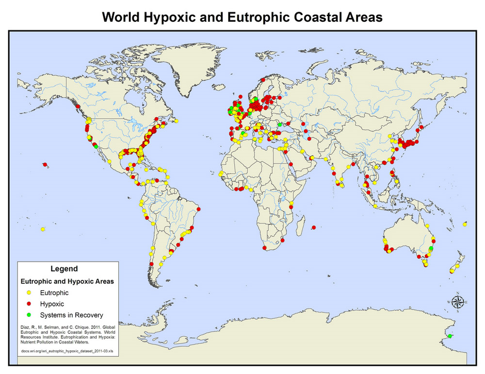
Warmists consistently do recycling, especially alarming stories coming back for encore media appearances. This week it’s the suffocating ocean meme, which taps into our caring about the seas, but conflates impacts from human maritime activities with subtle temperature changes, i.e climate change (AKA emergency, chaos, crisis etc.). Of course COP 25 is the trigger for this. I won’t list the alarming headlines since they are little different from last time, covered in a previous post reprinted below. Below are two typical recent quotes showing how an actual ocean concern is exploited for fossil fuel activism.
“A healthy ocean with abundant wildlife is capable of slowing the rate of climate breakdown substantially,” said Dr Monica Verbeek, the executive director of the group Seas at Risk. “To date, the most profound impact on the marine environment has come from fishing. Ending overfishing is a quick, deliverable action which will restore fish populations, create more resilient ocean ecosystems, decrease CO2 pollution and increase carbon capture, and deliver more profitable fisheries and thriving coastal communities.”
“Ending overfishing would strengthen the ocean, making it more capable of withstanding climate change and restoring marine ecosystems – and it can be done now,” explained Rashid Sumaila, professor and director of the fisheries economics research unit at the University of British Columbia. “The crisis in our fisheries and in our oceans and climate are not mutually exclusive problems to be addressed separately – it is imperative that we move forward with comprehensive solutions to address them.”
Previous post from last year
The climate scare machine is promoting again the fear of suffocating oceans. For example, an article this week by Chris Mooney in Washington Post, It’s Official, the Oceans are Losing Oxygen.
A large research synthesis, published in one of the world’s most influential scientific journals, has detected a decline in the amount of dissolved oxygen in oceans around the world — a long-predicted result of climate change that could have severe consequences for marine organisms if it continues.
The paper, published Wednesday in the journal Nature by oceanographer Sunke Schmidtko and two colleagues from the GEOMAR Helmholtz Centre for Ocean Research in Kiel, Germany, found a decline of more than 2 percent in ocean oxygen content worldwide between 1960 and 2010.
Climate change models predict the oceans will lose oxygen because of several factors. Most obvious is simply that warmer water holds less dissolved gases, including oxygen. “It’s the same reason we keep our sparkling drinks pretty cold,” Schmidtko said.
But another factor is the growing stratification of ocean waters. Oxygen enters the ocean at its surface, from the atmosphere and from the photosynthetic activity of marine microorganisms. But as that upper layer warms up, the oxygen-rich waters are less likely to mix down into cooler layers of the ocean because the warm waters are less dense and do not sink as readily.
And of course, other journalists pile on with ever more catchy headlines.
The World’s Oceans Are Losing Oxygen Due to Climate Change
How Climate Change Is Suffocating The Oceans
Overview of Oceanic Oxygen
Once again climate alarmists/activists have seized upon an actual environmental issue, but misdirect the public toward their CO2 obsession, and away from practical efforts to address a real concern. Some excerpts from scientific studies serve to put things in perspective.
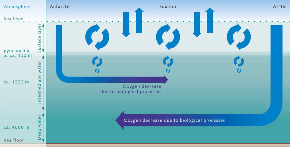
2.14 > Oxygen from the atmosphere enters the near-surface waters of the ocean. This upper layer is well mixed, and is thus in chemical equilibrium with the atmosphere and rich in O2. It ends abruptly at the pyncnocline, which acts like a barrier. The oxygenrich water in the surface zone does not mix readily with deeper water layers. Oxygen essentially only enters the deeper ocean by the motion of water currents, especially with the formation of deep and intermediate waters in the polarregions. In the inner ocean, marine organisms consume oxygen. This creates a very sensitive equilibrium.
How the Ocean Breathes
Variability in oxygen and nutrients in South Pacific Antarctic Intermediate Water by J. L. Russell and A. G. Dickson
The Southern Ocean acts as the lungs of the ocean; drawing in oxygen and exchanging carbon dioxide. A quantitative understanding of the processes regulating the ventilation of the Southern Ocean today is vital to assessments of the geochemical significance of potential circulation reorganizations in the Southern Hemisphere, both during glacial-interglacial transitions and into the future.
Traditionally, the change in the concentration of oxygen along an isopycnal due to remineralization of organic material, known as the apparent oxygen utilization (AOU), has been used by physical oceanographers as a proxy for the time elapsed since the water mass was last exposed to the atmosphere. The concept of AOU requires that newly subducted water be saturated with respect to oxygen and is calculated from the difference between the measured oxygen concentration and the saturated concentration at the sample temperature.
This study has shown that the ratio of oxygen to nutrients can vary with time. Since Antarctic Intermediate Water provides a necessary component to the Pacific equatorial biological regime, this relatively high-nutrient, high-oxygen input to the Equatorial Undercurrent in the Western Pacific plays an important role in driving high rates of primary productivity on the equator, while limiting the extent of denitrifying bacteria in the eastern portion of the basin.
Uncertain Measures of O2 Variability and Linkage to Climate Change
A conceptual model for the temporal spectrum of oceanic oxygen variability by Taka Ito and Curtis Deutsch
Changes in dissolved O2 observed across the world oceans in recent decades have been interpreted as a response of marine biogeochemistry to climate change. Little is known however about the spectrum of oceanic O2 variability. Using an idealized model, we illustrate how fluctuations in ocean circulation and biological respiration lead to low-frequency variability of thermocline oxygen.
Because the ventilation of the thermocline naturally integrates the effects of anomalous respiration and advection over decadal timescales, shortlived O2 perturbations are strongly damped, producing a red spectrum, even in a randomly varying oceanic environment. This background red spectrum of O2 suggests a new interpretation of the ubiquitous strength of decadal oxygen variability and provides a null hypothesis for the detection of climate change influence on oceanic oxygen. We find a statistically significant spectral peak at a 15–20 year timescale in the subpolar North Pacific, but the mechanisms connecting to climate variability remain uncertain.
The spectral power of oxygen variability increases from inter-annual to decadal frequencies, which can be explained using a simple conceptual model of an ocean thermocline exposed to random climate fluctuations. The theory predicts that the bias toward low-frequency variability is expected to level off as the forcing timescales become comparable to that of ocean ventilation. On time scales exceeding that of thermocline renewal, O2 variance may actually decrease due to the coupling between physical O2 supply and biological respiration [Deutsch et al., 2006], since the latter is typically limited by the physical nutrient supply.
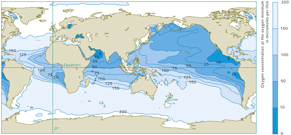
2.15 > Marine regions with oxygen deficiencies are completely natural. These zones are mainly located in the mid-latitudes on the west sides of the continents. There is very little mixing here of the warm surface waters with the cold deep waters, so not much oxygen penetrates to greater depths. In addition, high bioproductivity and the resulting large amounts of sinking biomass here lead to strong oxygen consumption at depth, especially between 100 and 1000 metres.
Climate Model Projections are Confounded by Natural Variability
Natural variability and anthropogenic trends in oceanic oxygen in a coupled carbon cycle–climate model ensemble by T. L. Frolicher et al.
Internal and externally forced variability in oceanic oxygen (O2) are investigated on different spatiotemporal scales using a six-member ensemble from the National Center for Atmospheric Research CSM1.4-carbon coupled climate model. The oceanic O2 inventory is projected to decrease significantly in global warming simulations of the 20th and 21st centuries.
The anthropogenically forced O2 decrease is partly compensated by volcanic eruptions, which cause considerable interannual to decadal variability. Volcanic perturbations in oceanic oxygen concentrations gradually penetrate the ocean’s top 500 m and persist for several years. While well identified on global scales, the detection and attribution of local O2 changes to volcanic forcing is difficult because of unforced variability.
Internal climate modes can substantially contribute to surface and subsurface O2 variability. Variability in the North Atlantic and North Pacific are associated with changes in the North Atlantic Oscillation and Pacific Decadal Oscillation indexes. Simulated decadal variability compares well with observed O2 changes in the North Atlantic, suggesting that the model captures key mechanisms of late 20th century O2 variability, but the model appears to underestimate variability in the North Pacific.
Our results suggest that large interannual to decadal variations and limited data availability make the detection of human-induced O2 changes currently challenging.
The concentration of dissolved oxygen in the thermocline and the deep ocean is a particularly sensitive indicator of change in ocean transport and biology [Joos et al., 2003]. Less than a percent of the combined atmosphere and ocean O2 inventory is found in the ocean. The O2 concentration in the ocean interior reflects the balance between O2 supply from the surface through physical transport and O2 consumption by respiration of organic material.
Our modeling study suggests that over recent decades internal natural variability tends to mask simulated century-scale trends in dissolved oxygen from anthropogenic forcing in the North Atlantic and Pacific. Observed changes in oxygen are similar or even smaller in magnitude than the spread of the ensemble simulation. The observed decreasing trend in dissolved oxygen in the Indian Ocean thermocline and the boundary region between the subtropical and subpolar gyres in the North Pacific has reversed in recent years [McDonagh et al., 2005; Mecking et al., 2008], implicitly supporting this conclusion.
The presence of large-scale propagating O2 anomalies, linked with major climate modes, complicates the detection of long-term trends in oceanic O2 associated with anthropogenic climate change. In particular, we find a statistically significant link between O2 and the dominant climate modes (NAO and PDO) in the North Atlantic and North Pacific surface and subsurface waters, which are causing more than 50% of the total internal variability of O2 in these regions.
To date, the ability to detect and interpret observed changes is still limited by lack of data. Additional biogeo-chemical data from time series and profiling floats, such as the Argo array (http://www.argo.ucsd.edu) are needed to improve the detection of ocean oxygen and carbon system changes and our understanding of climate change.
The Real Issue is Ocean Dead Zones, Both Natural and Man-made
Since 1994, he and the World Resources Institute (report here) in Washington,D.C., have identified and mapped 479 dead zones around the world. That’s more than nine times as many as scientists knew about 50 years ago.
What triggers the loss of oxygen in ocean water is the explosive growth of sea life fueled by the release of too many nutrients. As they grow, these crowds can simply use up too much of the available oxygen.
Many nutrients entering the water — such as nitrogen and phosphorus — come from meeting the daily needs of some seven billion people around the world, Diaz says. Crop fertilizers, manure, sewage and exhaust spewed by cars and power plants all end up in waterways that flow into the ocean. Each can contribute to the creation of dead zones.
Ordinarily, when bacteria steal oxygen from one patch of water, more will arrive as waves and ocean currents bring new water in. Waves also can grab oxygen from the atmosphere.
Dead zones develop when this ocean mixing stops.
Rivers running into the sea dump freshwater into the salty ocean. The sun heats up the freshwater on the sea surface. This water is lighter than cold saltier water, so it floats atop it. When there are not enough storms (including hurricanes) and strong ocean currents to churn the water, the cold water can get trapped below the fresh water for long periods.
Dead zones are seasonal events. They typically last for weeks or months. Then they’ll disappear as the weather changes and ocean mixing resumes.
Solutions are Available and do not Involve CO2 Emissions

Helping dead zones recover
The Black Sea is bordered by Europe and Asia. Dead zones used to develop here that covered an area as large as Switzerland. Fertilizers running off of vast agricultural fields and animal feedlots in the former Soviet Union were a primary cause. Then, in 1989, parts of the Soviet Union began revolting. Two years later, this massive nation broke apart into 15 separate countries.
The political instability hurt farm activity. In short order, use of nitrogen and phosphorus fertilizers by area farmers declined. Almost at once, the size of the Black Sea’s dead zone shrunk dramatically. Now if a dead zone forms there it’s small, Rabalais says. Some years there is none.
Chesapeake Bay, the United State’s largest estuary, has its own dead zone. And the area affected has expanded over the past 50 years due to pollution. But since the 1980s, farmers, landowners and government agencies have worked to reduce the nutrients flowing into the bay.
Farmers now plant cover crops, such as oats or barley, that use up fertilizer that once washed away into rivers. Growers have also established land buffers to absorb nutrient runoff and to keep animal waste out of streams. People have even started to use laundry detergents made without phosphorus.
In 2011, scientists reported that these efforts had achieved some success in shrinking the size of the bay’s late-summer dead zones.
The World Resources Institute lists 55 dead zones as improving. “The bottom line is if we take a look at what is causing a dead zone and fix it, then the dead zone goes away,” says Diaz. “It’s not something that has to be permanent.”
Summary
Alarmists/activists are again confusing the public with their simplistic solution for a complex situation. And actual remedies are available, just not the agenda preferred by climatists.

Waste Management Saves the Ocean