Climate Law Alaska Update


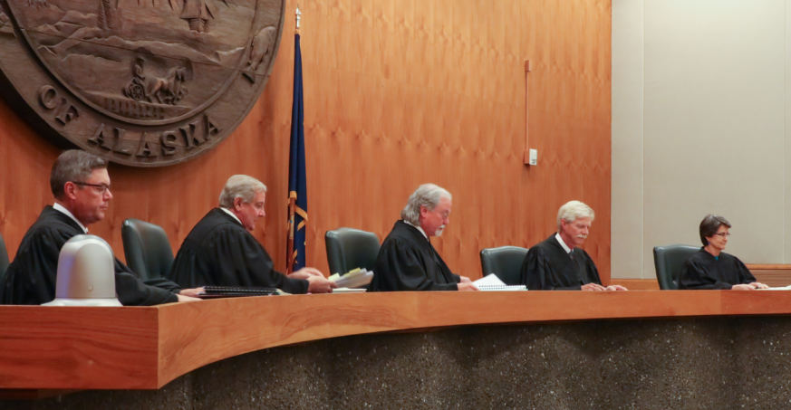
The Alaska Supreme Court hears arguments in the Boney Courthouse in Anchorage .

Our Children’s Trust is at it again. The activist legal organization with deep pockets recruits idealistic teenagers to front for lawsuits so that the courts will order governments to reduce CO2 emissions. The arena is again the Supreme Court of Alaska, a soft target since it is predisposed to hear cases from disgruntled citizens. More on the latest case later on.

And who are the adults involved in  Our Children’s Trust?

Supporting Experts (the usual suspects)

Dr. James Hansen
Dr. Ove Hoegh-Guldberg
Dr. Sivan Kartha
Dr. Pushker Kharecha
Dr. David Lobell
Dr. Arjun Makhijani
Dr. Jonathan Overpeck
Dr. Camille Parmeson
Dr. Stefan Rahmstorf
Dr. Steven Running
Dr. James Gustave Speth
Dr. Kevin Trenberth
Dr. Lise Van Susteren
Dr. Paul Epstein (1943-2011)
Etc

Campaign Partners (Allies whose funding depends on CO2 Hysteria)

Climate Reality Project,
Western Environmental Law Center,
Crag Law Center,
Texas Environmental Law Center,
Cottonwood Environmental Law Center,
WildEarth Guardians,
Clean Air Council,
Global Campaign for Climate Action,
Chasing Ice,
Environmental Law Alliance Worldwide,
TERRA,
Sierra Club,
350.org,
Climate Solutions,
Greenwatch,
Center for International Environmental Law..
Greenpeace
etc.

The Current Legal Skirmish

The October 27 news story is Young Alaskans sue the state, demanding action on climate change

Sixteen young Alaskans are suing the state, demanding Gov. Bill Walker’s administration take action on climate change.

It’s the second such legal action in the last six years. In 2014, the Alaska Supreme Court dismissed a similar lawsuit, Kanuk v Alaska, from six young people asking the state to reduce carbon emissions, among other recommendations. The justices ruled then that it’s not for the courts to set climate policy and that those decisions must be made through the political process, by the Legislature and the governor.

The new lawsuit says, essentially, the state has made its choice, and by encouraging oil development and permitting projects that emit greenhouse gases, Alaska is actively making climate change worse. The plaintiffs argue that violates their constitutional rights to, among other things, “a stable climate system that sustains human life and liberty.”

Alaska Court Not a Pushover

In 2014 the Alaska Supremes expressed respect for the youth while holding firmly to the law. Their reasoning is sound and adds to precedent against these attempts to legislate through the courts. From Alaska Supreme Court Opinion No sp-6953, Kanuk v Alaska (2014). Excerpts below with my bolds.

First Issue:  Do Plaintiffs have Legal Standing?

We recognize two types of standing: interest-injury standing and citizen taxpayer standing. The plaintiffs here claim interest-injury standing, which means they must show a “sufficient personal stake in the outcome of the controversy to ensure the requisite adversity.

Accepting these allegations as true and drawing all reasonable inferences in the plaintiffs’ favor, as courts are required to do on a motion to dismiss, we conclude that the complaint shows direct injury to a range of recognizable interests. Especially in light of our broad interpretation of standing and our policy of promoting citizen access to the courts, the plaintiffs’ allegations are sufficient to establish standing.

Second Issue: Are the Claims “Justiciable”?

Deciding whether a claim is justiciable depends on the answers to several questions. These include;
(1) whether deciding the claim would require us to answer questions that are better directed to the legislative or executive branches of government (the “political question” doctrine), and; 
(2) whether there are other reasons — such as ripeness, mootness, or standing — that persuade us that, though the case is one we are institutionally capable of deciding, prudence counsels that we not do so.

Among the plaintiffs’ claims in this case are requests that the superior court
(1) declare that the State’s obligation to protect the atmosphere be “dictated by best available science and that said science requires carbon dioxide emissions to peak in 2012 and be reduced by at least 6% each year until 2050”;
(2) order the State to reduce  emissions “by at least 6% per year from 2013 through at least 2050”; and
(3) order the State “to prepare a full and accurate accounting of Alaska’s current carbon dioxide emissions and to do so annually thereafter.”

We conclude that these three claims are non-justiciable under several of the Baker factors, most obviously the third: “the impossibility of deciding [them] without an initial policy determination of a kind clearly for nonjudicial discretion.”

While the science of anthropogenic climate change is compelling, government reaction to the problem implicates realms of public policy besides the objectively scientific. The legislature — or an executive agency entrusted with rule-making authority in this area — may decide that employment, resource development, power generation, health, culture, or other economic and social interests militate against implementing what the plaintiffs term the “best available science” in order to combat climate change.

We cannot say that an executive or legislative body that weighs the benefits and detriments to the public and then opts for an approach that differs from the plaintiffs’ proposed “best available science” would be wrong as a matter of law, nor can we hasten the regulatory process by imposing our own judicially created scientific standards. The underlying policy choices are not ours to make in the first instance.

This court, too, “lack[s] the scientific, economic, and technological resources an agency can utilize”; we too “are confined by [the] record” and “may not commission scientific studies or convene groups of experts for advice, or issue rules under notice-and-comment procedures.” The limited institutional role of the judiciary supports a conclusion that the science- and policy-based inquiry here is better reserved for executive branch agencies or the legislature, just as in AEP the inquiry was better reserved for the EPA.

Third Issue: Is a Declaratory Judgment Appropriate?

The remaining issue for us to address, therefore, is whether the plaintiffs’ claims for declaratory judgment — absent the prospect of any concrete relief — still present an “actual controversy” that is appropriate for our determination. We conclude they do not.

Applying these criteria here militates against granting the declaratory relief that the plaintiffs request. First, their request for a judgment that the State “has failed to uphold its fiduciary obligations” with regard to the atmosphere cannot be granted once the court has declined, on political question grounds, to determine precisely what those obligations entail.

As for the remaining claims — that the atmosphere is an asset of the public trust, with the State as trustee and the public as beneficiaries— the plaintiffs do make a good case. The Alaska Legislature has already intimated that the State acts as  trustee with regard to the air just as it does with regard to other natural resources. We note, however, that our past application of public trust principles has been as a restraint on the State’s ability to restrict public access to public resources, not as a theory for compelling regulation of those resources, as the plaintiffs seek to use it here.

Although declaring the atmosphere to be subject to the public trust doctrine could serve to clarify the legal relations at issue, it would certainly not “settle” them. It would have no immediate impact on greenhouse gas emissions in Alaska, it would not compel the State to take any particular action, nor would it protect the plaintiffs from the injuries they allege in their complaint. Declaratory relief would not tell the State what it needs to do in order to satisfy its trust duties and thus avoid future litigation; conversely it would not provide the plaintiffs any certain basis on which to determine in the future whether the State has breached its duties as trustee. In short, the declaratory judgment sought by the plaintiffs would not significantly advance the goals of “terminat[ing] and afford[ing] relief from the uncertainty, insecurity, and controversy giving rise to the proceeding” and would thus fail to serve the principal prudential goals of declaratory relief.

Scales of justice Alaska Commons

Conclusion

The Alaska Supreme Justices seem to be on their game, using their heads rather than succumbing to green threats, fears and prophecies.  But the whole charade is disgusting.

This is as obscene as brainwashing young Muslims to be suicide bombers. Or terrorists hiding among families to deter the drone strikes. The fact that the kids are willing is no excuse.

Think of the children! How will they feel a decade from now when they realize they have been duped and exploited by activists who figured judges would be more sympathetic to young believers?

Footnote for those not aware of Aliases for the Usual Suspects:

James “Death Trains” Hansen
Ove “Reefer Mad” Hoegh-Guldberg
Jonathan “Water Torture” Overpeck
Camille “The Extincter” Parmeson
Stefan “No Tommorow” Rahmstorf
Kevin “Hidden Heat” Trenberth

Arctic Seas Filling with Ice

click on image to enlarge.

Extents expanded rapidly during the last 12 days of October through yesterday, especially on the Eurasian side.   At the top center Laptev Sea fills in completely, and to the left East Siberian Sea is also growing solid ice toward East Asia. Kara sea on the right is growing fast ice from the shore outward, while Barents Sea fills in from the central Arctic.

The graph compares extents over the 28 days of October.
2017 has surpassed 8.1M km2, close to the 10 year average, and 700k km2 more than 2012.  2007 lags 925k km2 lower than 2017, while 2016 is 1M km2 behind.  At this point MASIE and SII are showing similar ice gains in October, tracking the 10-year average.

The Table below shows where ice is located on day 301 in regions of the Arctic ocean. 10 year average comes from 2007 through 2016 inclusive.

Region 2017301 Day 301
Average
2017-Ave. 2007301 2017-2007
 (0) Northern_Hemisphere 8144166 8170174 -26008 7217625 926541
 (1) Beaufort_Sea 866727 897500 -30773 933022 -66295
 (2) Chukchi_Sea 374051 451466 -77415 202567 171484
 (3) East_Siberian_Sea 915679 872509 43170 327344 588336
 (4) Laptev_Sea 897755 876350 21406 885761 11995
 (5) Kara_Sea 444927 384807 60120 243253 201674
 (6) Barents_Sea 99229 59612 39617 27244 71985
 (7) Greenland_Sea 280222 416824 -136602 433620 -153398
 (8) Baffin_Bay_Gulf_of_St._Lawrence 284534 221179 63355 179395 105139
 (9) Canadian_Archipelago 763764 754817 8947 739551 24213
 (10) Hudson_Bay 36124 66028 -29904 54271 -18147
 (11) Central_Arctic 3169661 3160785 8876 3190324 -20663

The deficits to average are mainly in Chukchi and Greenland Seas, while surpluses are large on Eurasian side from East Siberian, through Laptev, Kara and Barents.  Baffin Bay is also ahead of average.

Halloween is Coming!

Footnote

Some people unhappy with the higher amounts of ice extent shown by MASIE continue to claim that Sea Ice Index is the only dataset that can be used. This is false in fact and in logic. Why should anyone accept that the highest quality picture of ice day to day has no shelf life, that one year’s charts can not be compared with another year? Researchers do this analysis, including Walt Meier in charge of Sea Ice Index. That said, I understand his interest in directing people to use his product rather than one he does not control. As I have said before:

MASIE is rigorous, reliable, serves as calibration for satellite products, and uses modern technologies to continue the long and honorable tradition of naval ice charting.  More on this at my post Support MASIE Arctic Ice Dataset

Note:  Sea Ice Index (SII) is reporting extents according to version 3.0 as of October 20, 2017. Details at:
Sea Ice Index Updates to v.3.0

Footnote on MASIE Data Sources: 

National Ice Center (NIC) produces ice charts using the Interactive Multisensor Snow and Ice Mapping System (IMS). From the documentation, the multiple sources feeding IMS are:

Platform(s) AQUA, DMSP, DMSP 5D-3/F17, GOES-10, GOES-11, GOES-13, GOES-9, METEOSAT, MSG, MTSAT-1R, MTSAT-2, NOAA-14, NOAA-15, NOAA-16, NOAA-17, NOAA-18, NOAA-N, RADARSAT-2, SUOMI-NPP, TERRA

Sensor(s): AMSU-A, ATMS, AVHRR, GOES I-M IMAGER, MODIS, MTSAT 1R Imager, MTSAT 2 Imager, MVIRI, SAR, SEVIRI, SSM/I, SSMIS, VIIRS

Historical Summary: IMS Daily Northern Hemisphere Snow and Ice Analysis

The National Oceanic and Atmospheric Administration / National Environmental Satellite, Data, and Information Service (NOAA/NESDIS) has an extensive history of monitoring snow and ice coverage.Accurate monitoring of global snow/ice cover is a key component in the study of climate and global change as well as daily weather forecasting.

The Polar and Geostationary Operational Environmental Satellite programs (POES/GOES) operated by NESDIS provide invaluable visible and infrared spectral data in support of these efforts. Clear-sky imagery from both the POES and the GOES sensors show snow/ice boundaries very well; however, the visible and infrared techniques may suffer from persistent cloud cover near the snowline, making observations difficult (Ramsay, 1995). The microwave products (DMSP and AMSR-E) are unobstructed by clouds and thus can be used as another observational platform in most regions. Synthetic Aperture Radar (SAR) imagery also provides all-weather, near daily capacities to discriminate sea and lake ice. With several other derived snow/ice products of varying accuracy, such as those from NCEP and the NWS NOHRSC, it is highly desirable for analysts to be able to interactively compare and contrast the products so that a more accurate composite map can be produced.

The Satellite Analysis Branch (SAB) of NESDIS first began generating Northern Hemisphere Weekly Snow and Ice Cover analysis charts derived from the visible satellite imagery in November, 1966. The spatial and temporal resolutions of the analysis (190 km and 7 days, respectively) remained unchanged for the product’s 33-year lifespan.

As a result of increasing customer needs and expectations, it was decided that an efficient, interactive workstation application should be constructed which would enable SAB to produce snow/ice analyses at a higher resolution and on a daily basis (~25 km / 1024 x 1024 grid and once per day) using a consolidated array of new as well as existing satellite and surface imagery products. The Daily Northern Hemisphere Snow and Ice Cover chart has been produced since February, 1997 by SAB meteorologists on the IMS.

Another large resolution improvement began in early 2004, when improved technology allowed the SAB to begin creation of a daily ~4 km (6144×6144) grid. At this time, both the ~4 km and ~24 km products are available from NSIDC with a slight delay. Near real-time gridded data is available in ASCII format by request.

In March 2008, the product was migrated from SAB to the National Ice Center (NIC) of NESDIS. The production system and methodology was preserved during the migration. Improved access to DMSP, SAR, and modeled data sources is expected as a short-term from the migration, with longer term plans of twice daily production, GRIB2 output format, a Southern Hemisphere analysis, and an expanded suite of integrated snow and ice variable on horizon.

http://www.natice.noaa.gov/ims/ims_1.html


Global Ocean Cooling in September

September Sea Surface Temperatures (SSTs) are now available, and we see downward spikes in ocean temps everywhere, led by sharp decreases in the Tropics and SH, reversing the bump upward last month. The Tropical cooling in particular factors into forecasters favoring an unusually late La Nina appearance in coming months.

HadSST is generally regarded as the best of the global SST data sets, and so the temperature story here comes from that source, the latest version being HadSST3.

The chart below shows SST monthly anomalies as reported in HadSST3 starting in 2015 through September 2017.

The August bump upward was overcome with the Global average matching the lowest level in the chart at February 2015.  September NH temps almost erased a three-month climb; even so 9/2017 is well below the previous two years.  Meanwhile SH and the Tropics are setting new lows for this period.  With current reports from the El Nino 3.4 grid sector, it seems likely October will go even lower, with downward moves across all oceans.

Note that higher temps in 2015 and 2016 were first of all due to a sharp rise in Tropical SST, beginning in March 2015, peaking in January 2016, and steadily declining back to its beginning level. Secondly, the Northern Hemisphere added two bumps on the shoulders of Tropical warming, with peaks in August of each year. Also, note that the global release of heat was not dramatic, due to the Southern Hemisphere offsetting the Northern one.

Note:  Last month someone asked about HadSST calculations, especially as the Global appeared to be a simple average of NH and SH, which would be misleading.  My queries to Met Office received these clarifying responses:

My colleague in the Climate Monitoring and Research team has advised the following:

For HadSST3, we take an area-weighted average of all the grid boxes with data in to calculate the global average. We don’t calculate the two hemispheric series and then average them. In the case of SST, this wouldn’t work because the southern hemisphere ocean area is larger than the northern hemisphere.

The uncertainty that arises from incomplete sampling is estimated and incorporated into the global average SST files. Coverage varies throughout the record with the northern hemisphere being generally better observed, but at other times, coverage is concentrated other places, dictated by where shipping happened to be at those times. Since the mid 2000s drifting buoys have provided a more uniform sampling of the world’s oceans. When we compare to other data sets, we typically compare where both data sets have data which minimizes the coverage problems.

Kind regards,  Misha,  Weather Desk Climate Advisor

Summary

We have seen lots of claims about the temperature records for 2016 and 2015 proving dangerous man made warming.  At least one senator stated that in a confirmation hearing.  Yet HadSST3 data for the last two years show how obvious is the ocean’s governing of global average temperatures.

USS Pearl Harbor deploys Global Drifter Buoys in Pacific Ocean

The best context for understanding these two years comes from the world’s sea surface temperatures (SST), for several reasons:

  • The ocean covers 71% of the globe and drives average temperatures;
  • SSTs have a constant water content, (unlike air temperatures), so give a better reading of heat content variations;
  • A major El Nino was the dominant climate feature these years.

Solar energy accumulates massively in the ocean and is variably released during circulation events.


Bonn COP23 Briefing for Realists


STEPHANE KIEHL POUR “LE MONDE”

French Mathematicians spoke out prior to COP21 in Paris, and their words provide a rational briefing for COP23 beginning in Bonn next month.  In a nutshell:

Fighting Global Warming is Absurd, Costly and Pointless.

  • Absurd because of no reliable evidence that anything unusual is happening in our climate.
  • Costly because trillions of dollars are wasted on immature, inefficient technologies that serve only to make cheap, reliable energy expensive and intermittent.
  • Pointless because we do not control the weather anyway.

The prestigious Société de Calcul Mathématique (Society for Mathematical Calculation) issued a detailed 195-page White Paper that presents a blistering point-by-point critique of the key dogmas of global warming. The synopsis is blunt and extremely well documented.  Here are extracts from the opening statements of the first three chapters of the SCM White Paper with my bolds and images.

Sisyphus at work.

Chapter 1: The crusade is absurd
There is not a single fact, figure or observation that leads us to conclude that the world‘s climate is in any way ‘disturbed.’ It is variable, as it has always been, but rather less so now than during certain periods or geological eras. Modern methods are far from being able to accurately measure the planet‘s global temperature even today, so measurements made 50 or 100 years ago are even less reliable. Concentrations of CO2 vary, as they always have done; the figures that are being released are biased and dishonest. Rising sea levels are a normal phenomenon linked to upthrust buoyancy; they are nothing to do with so-called global warming. As for extreme weather events — they are no more frequent now than they have been in the past. We ourselves have processed the raw data on hurricanes….

Chapter 2: The crusade is costly
Direct aid for industries that are completely unviable (such as photovoltaics and wind turbines) but presented as ‘virtuous’ runs into billions of euros, according to recent reports published by the Cour des Comptes (French Audit Office) in 2013. But the highest cost lies in the principle of ‘energy saving,’ which is presented as especially virtuous. Since no civilization can develop when it is saving energy, ours has stopped developing: France now has more than three million people unemployed — it is the price we have to pay for our virtue….

Chapter 3: The crusade is pointless
Human beings cannot, in any event, change the climate. If we in France were to stop all industrial activity (let’s not talk about our intellectual activity, which ceased long ago), if we were to eradicate all trace of animal life, the composition of the atmosphere would not alter in any measurable, perceptible way. To explain this, let us make a comparison with the rotation of the planet: it is slowing down. To address that, we might be tempted to ask the entire population of China to run in an easterly direction. But, no matter how big China and its population are, this would have no measurable impact on the Earth‘s rotation.

Full text in pdf format is available in English at link below:

The battle against global warming: an absurd, costly and pointless crusade
White Paper drawn up by the Société de Calcul Mathématique SA
(Mathematical Modelling Company, Corp.)

A Second report was published in 2016 entitled: Global Warming and Employment, which analyzes in depth the economic destruction from ill-advised climate change policies.

The two principal themes are that jobs are disappearing and that the destructive forces are embedded in our societies.

Jobs are Disappearing discusses issues such as:

The State is incapable of devising and implementing an industrial policy.

The fundamental absurdity of the concept of sustainable development

Biofuels an especially absurd policy leading to ridiculous taxes and job losses.

EU policy to reduce greenhouse gas emissions by 40% drives jobs elsewhere while being pointless: the planet has never asked for it, is completely unaware of it, and will never notice it!

The War against the Car and Road Maintenance undercuts economic mobility while destroying transportation sector jobs.

Solar and wind energy are weak, diffuse, and inconsistent, inadequate to power modern civilization.

Food production activities are attacked as being “bad for the planet.”

So-called Green jobs are entirely financed by subsidies.

The Brutalizing Whip discusses the damages to public finances and to social wealth and well-being, including these topics:

Taxes have never been so high

The Government is borrowing more and more

Dilapidated infrastructure

Instead of job creation, Relocations and Losses

The wastefulness associated with the new forms of energy

Return to the economy of an underdeveloped country

What is our predicament?
Four Horsemen are bringing down our societies:

  • The Ministry of Ecology (climate and environment);
  • Journalists;
  • Scientists;
  • Corporation Environmentalist Departments.

Steps required to recover from this demise:

  • Go back to the basic rules of research.
  • Go back to the basic rules of law
  • Do not trust international organizations
  • Leave the planet alone
  • Beware of any premature optimism

Conclusion

Climate lemmings

The real question is this: how have policymakers managed to make such absurd decisions, to blinker themselves to such a degree, when so many means of scientific investigation are available? The answer is simple: as soon as something is seen as being green, as being good for the planet, all discussion comes to an end and any scientific analysis becomes pointless or counterproductive. The policymakers will not listen to anyone or anything; they take all sorts of hasty, contradictory, damaging and absurd decisions. When will they finally be held to account?

Footnote:

The above cartoon image of climate talks includes water rising over politicians’ feet.  But actual observations made in Fiji (presiding over these talks in Bonn) show sea levels are stable (link below).

Fear Not For Fiji

Snowing and Freezing in the Arctic

The image from IMS shows snow and ice on day 296 (yesterday) 2007 to 2017, with focus on Eurasia but also showing Canada and Alaska.  You can see that low Arctic ice years, like 2007, 2012 and 2016 have a smaller snow extent on both sides of the Arctic.  Conversely, higher Arctic ice years like 2013, 2014 and 2015 show snow spreading into northern Europe, as well as Alaska.  The pattern appears as gaining snow and ice 2008 to 10, losing 2011 and 2012, then regaining 2013 to 15, before retreating in 2016.  So far 2017 is looking more like 2013 to 15.

From Post Natural Climate Factors: Snow 

Previously I posted an explanation by Dr. Judah Cohen regarding a correlation between autumn Siberian snow cover and the following winter conditions, not only in the Arctic but extending across the Northern Hemisphere. More recently, in looking into Climate Model Upgraded: INMCM5, I noticed some of the scientists were also involved in confirming the importance of snow cover for climate forecasting. Since the poles function as the primary vents for global cooling, what happens in the Arctic in no way stays in the Arctic. This post explores data suggesting changes in snow cover drive some climate changes.

The Snow Cover Climate Factor

The diagram represents how Dr. judah Cohen pictures the Northern Hemisphere wintertime climate system.  He leads research regarding Arctic and NH weather patterns for AER.

cohen-schematic2

Dr. Cohen explains the mechanism in this diagram.

Conceptual model for how fall snow cover modifies winter circulation in both the stratosphere and the troposphere–The case for low snow cover on left; the case for extensive snow cover on right.

1. Snow cover increases rapidly in the fall across Siberia, when snow cover is above normal diabatic cooling helps to;
2. Strengthen the Siberian high and leads to below normal temperatures.
3. Snow forced diabatic cooling in proximity to high topography of Asia increases upward flux of energy in the troposphere, which is absorbed in the stratosphere.
4. Strong convergence of WAF (Wave Activity Flux) indicates higher geopotential heights.
5. A weakened polar vortex and warmer down from the stratosphere into the troposphere all the way to the surface.
6. Dynamic pathway culminates with strong negative phase of the Arctic Oscillation at the surface.

From Eurasian Snow Cover Variability and Links with Stratosphere-Troposphere
Coupling and Their Potential Use in Seasonal to Decadal Climate Predictions by Judah Cohen.

Variations in Siberian snow cover October (day 304) 2004 to 2016. Eurasian snow charts from IMS.

Observations of the Snow Climate Factor

For several decades the IMS snow cover images have been digitized to produce a numerical database for NH snow cover, including area extents for Eurasia. The NOAA climate data record of Northern Hemisphere snow cover extent, Version 1, is archived and distributed by NCDC’s satellite Climate Data Record Program. The CDR is forward processed operationally every month, along with figures and tables made available at Rutgers University Global Snow Lab.

This first graph shows the snow extents of interest in Dr. Cohen’s paradigm. The Autumn snow area in Siberia is represented by the annual Eurasian averages of the months of October and November (ON). The following NH Winter is shown as the average snow area for December, January and February (DJF). Thus the year designates the December of that year plus the first two months of the next year.

Notes: NH snow cover minimum was 1981, trending upward since.  Siberian autumn snow cover was lowest in 1989, increasing since then.  Autumn Eurasian snow cover is about 1/3 of Winter NH snow area. Note also that fluctuations are sizable and correlated.

The second graph presents annual anomalies for the two series, each calculated as the deviation from the mean of its entire time series. Strikingly, the Eurasian Autumn flux is on the same scale as total NH flux, and closely aligned. While NH snow cover declined a few years prior to 2016, Eurasian snow is trending upward strongly.  If Dr. Cohen is correct, NH snowfall will follow. The linear trend is slightly positive, suggesting that fears of children never seeing snowfall have been exaggerated. The Eurasian trend line (not shown) is almost the same.

What About Winter 2017-2018?

These data confirm that Dr. Cohen and colleagues are onto something. Here are excerpts from his October 2 outlook for the upcoming season AER. (my bolds)

The main block/high pressure feature influencing Eurasian weather is currently centered over the Barents-Kara Seas and is predicted to first weaken and then strengthen over the next two weeks.

Blocking in the Barents-Kara Seas favors troughing/negative geopotential height anomalies and cool temperatures downstream over Eurasia but especially Central and East Asia. The forecast for the next two weeks across Central Asia is for continuation of overall below normal temperatures and new snowfall.

Currently the largest negative anomalies in sea ice extent are in the Chukchi and Beaufort Seas but that will change over the next month or so during the critical months of November-February. In my opinion low Arctic sea ice favors a more severe winter but not necessarily hemisphere-wide and depends on the regions of the strongest anomalies. Strong negative departures in the Barents-Kara Seas favors cold temperatures in Asia while strong negative departures near Greenland and/or the Beaufort Sea favor cold temperatures in eastern North America.

Siberian snow cover is advancing quickly relative to climatology and is on a pace similar to last year at this time. My, along with my colleagues and others, research has shown that extensive Siberian snow cover in the fall favors a trough across East Asia with a ridge to the west near the Urals. The atmospheric circulation pattern favors more active poleward heat flux, a weaker PV and cold temperatures across the NH. It is very early in the snow season but recent falls have been snowy across Siberia and therefore I do expect another upcoming snowy fall across Siberia.

Summary

In summary the three main predictors that I follow in the fall months most closely, the presence or absence of high latitude blocking, Arctic sea ice extent and Siberian snow cover extent all point towards a more severe winter across the continents of the NH.

Uh oh.  Now where did I put away my long johns?

Fear Not For Fiji

Fiji Map from Turtle Airways Seaplanes. Fiji International Airport is at Nadi.

Published this month is an update on sea levels at Fiji, and thankfully the threat level can be dialed way down.  (H/T Tallbloke)  The Research Article:  Our Oceans-Our Future: New Evidence-based Sea Level Records from the Fiji Islands for the Last 500 years Indicating Rotational Eustasy and Absence of a Present Rise in Sea Level by Nils-Axel Mörner, Paleogeophysics & Geodynamics, Stockholm, Sweden. Excerpts with my bolds.

Update Feb. 17 at bottom

Abstract:

Previously, no study in the Fiji Islands had been devoted to the sea level changes of the last 500 years. No serious prediction can be made unless we have a good understanding of the sea level changes today and in the past centuries. Therefore, this study fills a gap, and provides real observational facts to assess the question of present sea level changes.

There is a total absence of data supporting the notion of a present sea level rise; on the contrary all available facts indicate present sea level stability. On the centennial timescale, there was a +70 cm high level in the 16th and 17th centuries, a -50 cm low in the 18th century and a stability (with some oscillations) in the 19th, 20th and early 21st centuries. This is almost identical to the sea level change documented in the Maldives, Bangladesh and Goa (India).

This seems to indicate a mutual driving force. However, the recorded sea level changes are anti-correlated with the major changes in climate during the last 600 years. Therefore, glacial eustasy cannot be the driving force. The explanation seems to be rotational eustasy with speeding-up phases during Grand Solar Minima forcing ocean water masses to the equatorial region, and slowing-down phases during Grand Solar Maxima forcing ocean waster massed from the equator towards the poles.

Background

The Intergovernmental Panel on Climate Change [1] has claimed that sea level is rising and that an additional acceleration is soon to be expected as a function of global warming. This proposition only works if the present warming would be a function of increased CO2 content in the atmosphere (an hypothesis termed AGW from Anthropogenic Global Warming). On a longer-term basis, it seems quite clear, however, that the dominant factor of global changes in temperature is changes in solar variability [2-3]. Regardless of what actually is driving climate change and sea level changes, the proposition of a rapidly rising sea level grew to a mantra in media and politics. This initiated a flood of papers rather based on models and statistics, however, than on actual field observations.

The Fiji government will be the chair-nation at the next international climate conference; COP23 in Bonn in November 2017 [4].  This paper represents a detailed analysis of available field  observation on sea level changes in the Fiji Islands over the last 500 Years.

Figure 1.

Sea level changes as documented in the Yasawa Islands, Fiji, composed of 3 main segments: a high level (1), a low level (2) and a more or less constant level (3), which might be subdivided in an early high level, a main level just above the present level and a lowering to the present level generating microatoll growth in the last 60 years (based on data from [13]). (Subdivisions shown in Figure 3 below)

Figure 2.

The long-term changes during the last 500 years – i.e. a high, a low and a present level – is recorded in the Maldives [16], in Bangladesh [17-18] and in Goa, India, [15,18], as illustrated in Figure 3. A present long-term stability is also recorded in Qatar [19].

Figure 3.

The general agreement between the observed sea level changes in Fiji during the last 500 years, and those recorded in the three Indian Ocean sites: the Maldives, Goa and Bangladesh is striking, which is a very strong (even conclusive) argument that the recorded sea level change are of regional eustatic origin [20].

All four records show a high in the 17th century (which was a period of Little Ice Age conditions), a low in the 18th century (which was a period nearly as warm as today) and a high in the early 19th century (which was the last period of Little Ice Age conditions). This means that the Figure 3 sea level changes are almost directly opposite to the general changes in global climate. Consequently, the eustatic changes recorded cannot refer to glacial eustasy, but must be understood in terms of rotational eustasy.

Figure 4

This calls for some explanation. The idea that oceanic water masses may be dislocated horizontally by rotational–dynamical forces was launched in 1984 [21] and more extensively presented in 1988 [22].  Later, is was proposed that changes in the Solar Wind strongly affects the Earth’s rate of rotation [23] (with a deeper analysis in [24]) leading to a beat in the Gulf Stream with alternations between a dominant northeastward flow during rotational slowing-down periods of Grand Solar Maxima, and dominant east-south eastward flow during rotational seeding-up periods of Grand Solar Minima [25].

The sea level changes in the Indian Ocean, were therefore proposed [26,15] to be driven by rotational eustasy; i.e. the interchanges of water masses between high-latitudes and the equatorial region as a function of the speeding-up during Grand Solar Minima with Little Ice Age conditions and slowing down during Grand Solar Maxima with generally warm climatic conditions.

In the post-Little Ice Ages period from 1850 up to 1930-1940 there was a global glacial eustatic rise in the order of 11 cm [28]. For the rest of the last 500 years, rotational eustasy seems to have been the dominant factor as documented in Figure 3 and illustrated in Figure 4.

CONCLUSIONS

(1)– sea level is not at all in a rising mode in the Fiji area
(2) – on the contrary it has remained stable in the last 50-70 years
(3) – rotational eustasy has dominated the sea level changes in Fiji
(4) – the same changes are recorded in the Indian Ocean

Previously, the changes in sea level during the last 500 years were not covered by adequate research in the Fiji Islands. The present paper provides a detailed analyses documenting a +70 cm high level in the 16th and 17th centuries, a -50 cm low in the 18th century and a period of virtually stability in the 19th to early 21st centuries, the last period of which may be subdivided into an early 19th century +30 cm high, a long period of stability and a 10-20 cm fall in sea level in the last 60 years forcing corals to grew into microatolls under strictly stable sea level conditions. This means there are no traces of a present rise in sea level; on the contrary: full stability.

The long-term trend is almost identical to the trends documented in the Indian Ocean in the Maldives, Goa and Bangladesh. This implies a eustatic origin of the changes recorded; not of glacial eustatic origin, however, but of rotational eustatic origin. The rotational eustatic changes in sea level are driven by the alternations of speeding-up during Grand Solar Minima (the Maunder and Dalton Solar Minima) forcing water towards the equator, and slowing-down during Grand Solar Maxima (in the 18th century, around 1930-1940 and at about 1970-2000).

Update Feb. 17

Prompted by a question from hunter, I found this informative recent letter on this topic (my bolds):

From Reply from Nils-Axel Mörner on the problems of estimating Future Sea Level Changes as asked by Albert Parker in letter of January 2, 2018

There are physical frames to consider. Ice melting requires time and heating, strictly bounded by physical laws. At the largest climatic jump in the last 20,000 years – viz. at the Pleistocene/Holocene boundary about 11,000 years BP – ice melted under extreme temperature forcing; still sea level only rose at a rate of about 10 mm/yr (or just a little more if one would consider more extreme eustatic reconstructions). Today, under interglacial climatic conditions with all the glacial ice caps gone climate forcing can only rise global sea level by a fraction of the 11,000 BP rate, which in comparison with the values of Garner et al. [1] would imply:
well below 0.4 m at 2050 instead of +0.6 m
well below 0.9 m at 2100 instead of +2.6 m
well below 2.9 m at 2300 instead of +17.5 m

Consequently, the values given by Garner et al. [1] violate physical laws and common glaciological knowledge. Therefore, their values must not be set as standard in coastal planning (point 2 above).

The mean sea level rise over the last 125 years is +0.81 ±0.18 mm/yr. At Stockholm in Sweden, the absolute uplift over the last 3000 years is strictly measured at +4.9 mm/yr. The mean tide-gauge change is -3.8 mm/yr, giving a eustatic component of +1.1 mm/yr for the last 150 years. In Amsterdam, the long-term subsidence is known as +0.4 mm/yr. The Amsterdam/Ijmuiden stations record a relative rise of +1.5 mm/yr, which give a eustatic component of +1.1 mm/yr.

Global Loading Adjustment has been widely used in order to estimate global sea level changes. Obviously, the globe must adjust its rate of rotation and geoid relief in close agreement with the glacial eustatic rise in sea level after the last Ice Age. The possible internal glacial loading adjustment is much more complicated, and even questionable, however.

Direct coastal analysis of morphology, stratigraphy, biological criteria, coastal dynamics, etc usually offers the far best means of recording the on-going sea level variations in a correct and meaningful way. It calls for hard work in the field and deep knowledge in a number of subjects. We have, very successfully, applied it in the Maldives, in Bangladesh, in Goa in southern India, and now also in the Fiji Islands. In all these sites, direct coastal analyses indicate full eustatic stability over the last 50-70 years, and long-term variations over the last 500 years that are consistent with “rotational eustasy” or “Global Solar Cycle Oscillations” (GSCO).


Arctic October Chill Continues

Extents expanded rapidly during the last 13 days of October through yesterday, already gaining back to  reach 50% of March maximum.   On the right side Laptev Sea has filled in completely, and just above it East Siberian Sea is also growing solid ice toward East Asia. Kara sea just below Laptev is growing fast ice from the shore outward. On the left, Canadian Archipelago is now full of ice, with Beaufort spreading toward shore and next to Greenland, Baffin Bay is extending southward.

The graph compares extents over the first 22 days of October.
2017 has reached 7.5 M km2, 100k km2 above the 10 year average, 800k km2 more than 2016 and more than 2012.  2007 lags 1.3M km2 lower than 2017.  At this point MASIE and SII are showing similar ice gains in October, tracking the 10-year average.

The Table below shows where ice is located on day 295 in regions of the Arctic ocean. 10 year average comes from 2007 through 2016 inclusive.

Region 2017295 Day 295
Average
2017-Ave. 2007295 2017-2007
 (0) Northern_Hemisphere 7543438 7431370 112068 6284693 1258745
 (1) Beaufort_Sea 764794 801247 -36453 806764 -41970
 (2) Chukchi_Sea 297001 378182 -81180 135321 161680
 (3) East_Siberian_Sea 737817 777926 -40109 133466 604351
 (4) Laptev_Sea 895187 725836 169351 690628 204559
 (5) Kara_Sea 365187 292669 72518 283333 81854
 (6) Barents_Sea 67973 47903 20070 25377 42597
 (7) Greenland_Sea 243447 401693 -158246 446006 -202559
 (8) Baffin_Bay_Gulf_of_St._Lawrence 224104 145178 78926 90620 133484
 (9) Canadian_Archipelago 747134 680155 66980 576142 170992
 (10) Hudson_Bay 39910 25325 14585 1954 37957
 (11) Central_Arctic 3158019 3151075 6944 3093807 64212

The important deficits to average are in Chukchi and Greenland Seas, while larger surpluses appear in Laptev, Kara, Baffin Bay and Canadian Archipelago. If ice extents continue to grow at the present rate to month end, the October 2017 monthly average will exceed the 10 year October average by several 100k km2.

Halloween is Coming!

Footnote

Some people unhappy with the higher amounts of ice extent shown by MASIE continue to claim that Sea Ice Index is the only dataset that can be used. This is false in fact and in logic. Why should anyone accept that the highest quality picture of ice day to day has no shelf life, that one year’s charts can not be compared with another year? Researchers do this analysis, including Walt Meier in charge of Sea Ice Index. That said, I understand his interest in directing people to use his product rather than one he does not control. As I have said before:

MASIE is rigorous, reliable, serves as calibration for satellite products, and uses modern technologies to continue the long and honorable tradition of naval ice charting.  More on this at my post Support MASIE Arctic Ice Dataset

Note:  Sea Ice Index (SII) is reporting extents according to version 3.0 as of October 20, 2017. Details at:
Sea Ice Index Updates to v.3.0

Footnote on MASIE Data Sources: 

National Ice Center (NIC) produces ice charts using the Interactive Multisensor Snow and Ice Mapping System (IMS). From the documentation, the multiple sources feeding IMS are:

Platform(s) AQUA, DMSP, DMSP 5D-3/F17, GOES-10, GOES-11, GOES-13, GOES-9, METEOSAT, MSG, MTSAT-1R, MTSAT-2, NOAA-14, NOAA-15, NOAA-16, NOAA-17, NOAA-18, NOAA-N, RADARSAT-2, SUOMI-NPP, TERRA

Sensor(s): AMSU-A, ATMS, AVHRR, GOES I-M IMAGER, MODIS, MTSAT 1R Imager, MTSAT 2 Imager, MVIRI, SAR, SEVIRI, SSM/I, SSMIS, VIIRS

Historical Summary: IMS Daily Northern Hemisphere Snow and Ice Analysis

The National Oceanic and Atmospheric Administration / National Environmental Satellite, Data, and Information Service (NOAA/NESDIS) has an extensive history of monitoring snow and ice coverage.Accurate monitoring of global snow/ice cover is a key component in the study of climate and global change as well as daily weather forecasting.

The Polar and Geostationary Operational Environmental Satellite programs (POES/GOES) operated by NESDIS provide invaluable visible and infrared spectral data in support of these efforts. Clear-sky imagery from both the POES and the GOES sensors show snow/ice boundaries very well; however, the visible and infrared techniques may suffer from persistent cloud cover near the snowline, making observations difficult (Ramsay, 1995). The microwave products (DMSP and AMSR-E) are unobstructed by clouds and thus can be used as another observational platform in most regions. Synthetic Aperture Radar (SAR) imagery also provides all-weather, near daily capacities to discriminate sea and lake ice. With several other derived snow/ice products of varying accuracy, such as those from NCEP and the NWS NOHRSC, it is highly desirable for analysts to be able to interactively compare and contrast the products so that a more accurate composite map can be produced.

The Satellite Analysis Branch (SAB) of NESDIS first began generating Northern Hemisphere Weekly Snow and Ice Cover analysis charts derived from the visible satellite imagery in November, 1966. The spatial and temporal resolutions of the analysis (190 km and 7 days, respectively) remained unchanged for the product’s 33-year lifespan.

As a result of increasing customer needs and expectations, it was decided that an efficient, interactive workstation application should be constructed which would enable SAB to produce snow/ice analyses at a higher resolution and on a daily basis (~25 km / 1024 x 1024 grid and once per day) using a consolidated array of new as well as existing satellite and surface imagery products. The Daily Northern Hemisphere Snow and Ice Cover chart has been produced since February, 1997 by SAB meteorologists on the IMS.

Another large resolution improvement began in early 2004, when improved technology allowed the SAB to begin creation of a daily ~4 km (6144×6144) grid. At this time, both the ~4 km and ~24 km products are available from NSIDC with a slight delay. Near real-time gridded data is available in ASCII format by request.

In March 2008, the product was migrated from SAB to the National Ice Center (NIC) of NESDIS. The production system and methodology was preserved during the migration. Improved access to DMSP, SAR, and modeled data sources is expected as a short-term from the migration, with longer term plans of twice daily production, GRIB2 output format, a Southern Hemisphere analysis, and an expanded suite of integrated snow and ice variable on horizon.

http://www.natice.noaa.gov/ims/ims_1.html


Wind Farms Make Climate Change

This just in from Dr. Arnd Bernaerts: Off shore wind farm impact is not natural variability
Article below with my bolds.

Climatology considers ‘natural variability’ as a valuable factor in climate change matters. Ignoring any human role in this respect is irresponsible. The latest big issue is floating off shore wind turbines with a structure about 78 meters submerged and 15 meters in diameters. Although a massive obstacle in a permanent moving marine environment the impact and change in ‘natural variability’ in climate change matters is completely ignored.

The concern has been raised in a recent post: ”Why Europe is warming up faster than elsewhere?” The matter is simple. Off shore installations affect sea temperatures and salinity structure at many locations to about 60 meters below the sea surface. In Europe the number of off shore wind turbines will account 4000 by the end of 2017. The inevitable consequence is at hand: “Northern European winters are getting warmer and warmer at a rate higher than global average” as analyzed in a paper by A. Bernaerts (2016).

(Note: Sections 1 to 4 are profiles at different latitudes of the North Sea, identified in map upper right corner.)

Now the impact on sea level structure increase further. The world’s first floating wind farm opened on 18 October 2017, off the east coast of Scotland. The 6MW turbines rise 175m above sea level, and extend 78m below the surface of the water, tied to the sea bed by cables. The anchors used to stabilize the turbines stand at 16m and weigh 111 tons. (Details) Inevitable huge water masses of different temperature and salinity will change between the various sea levels. As an example see Fig. 2 (Northern North Sea – Section 1-4). The sea surface will warm or cool and either warm or cool the air temperature above the scene.

Any use of the oceans by mankind has an influence on thermo-haline structures within the water column from a few cm to 10m and more. Not even raising and investigating this mechanism is a demonstration that the term “natural variability” is used to hide pseudoscience.

___A. Bernaerts (2016), Offshore Wind-Parks and Northern Europe’s Mild Winters: Contribution from Ships, Fishery, et cetera? Journal of Shipping and Ocean Engineering 6, p. 46-56, PDF HERE


Sea Ice Index Updates to v.3.0

In October 2012 Arctic sea ice doubled in extent.

As of October 20, 2017, NOAA@NSIDC Releases Sea Ice Index, Version 3.0

Text below from SII webpage explains the changes in versions.

NOAA@NSIDC is pleased to announce the release of Sea Ice Index Version 3 (V3). V3 changes the way the monthly average area and extent data values are calculated. The way monthly average area and extent images are created remains the same as in V2. All daily data remain the same as in V2.

The V3 method simply averages daily extent values, while the V2 method derived monthly average values from the gridded monthly-average concentration field. The change is in response to questions about what seemed to be an inconsistency between daily and monthly values. When users summed daily values, and then divided by number of days in a month to get a monthly average value, that number was different, and sometimes quite different, from the monthly average numbers we presented. Both the V2 and V3 methodologies are valid and defensible ways of representing passive microwave-derived sea ice concentration data, but the goal of this change is to better match the understanding of the user community as the product evolves through time.

Values will change slightly. V3 monthly average areas are slightly greater than those from V2. Conversely, V3 monthly average extents are slightly less than V2. Trends will change slightly as well. These are small changes, as the following images for March, over the entire time series, illustrate. Extent is on the left and area is on the right. Windnagel et al. (2017) offers additional analysis on why V3 areas are higher than V2 and V3 extents are lower than V2, along with a simple example. With the update to V3, there are no considerable differences in conclusions that can be made about the overall trends in sea ice area or extent.

Details are in this report: Sea Ice Index Version 3 Analysis. NSIDC Special Report 19.

The Sea Ice Index version 3 dataset is available here

Background:

Several posts at this blog compare results from MASIE and SII. Walt Meier, head of Sea Ice Index (SII) and colleagues did a comparison of the two datasets, published in October 2015. SII went from version 1 to v.2 in 2016, and then in January 2017 from v.2.0 to v.2.1, with some changes in past values.

One of the biggest discrepancies in the past with previous SII versions arose in the Month of October, and it is timely that version 3.0 appears now. The dataset is now available with past calculations according to v3, and the past can be compared in advance of 2017 monthly results.

For comparison, the graphs below show October monthly averages for MASIE compared to SII v.2 and SII v.3., 2007 through 2016.

Click on image to enlarge.

It seems clear that SIIv.3 is a big improvement relative to MASIE. And as well, October 2017 results are coming in with the two datasets tracking quite closely.

MASIE: “high-resolution, accurate charts of ice conditions”
Walt Meier, NSIDC, October 2015 article in Annals of Glaciology.

Earth Climate Layers

Thanks to No Tricks Zone for posting work (here) by Dr. Dai Davies of Canberra. In his writing I found a fine summary paradigm leading to the image above.  This post presents a scientifically rigorous view of our planetary climate system, starting with an airless rocky surface and then conceptually adding the dynamic elements in layers.  The text below with my bolds and images comes from Energy and Atmosphere by Dr. Dai Davies of University of Canberra,  Website: http://brindabella.id.au/climarc/.

The Earth’s atmosphere in stages

This is an hypothetical scenario that allows us to build up a picture, step by step, of how having an atmosphere can influence a planet.

Baseline: Airless, Rocky Planet
As a starting point we consider how the Earth’s temperature might vary through the daily cycle if it was an airless, rocky planet much like the moon. During the day, the sun heats up a surface layer of the rock which cools through infrared radiation. The temperature follows the sun’s irradiation almost directly, rising and plunging over a range of hundreds of degrees.

Add: Radiatively Inert Atmosphere
If we add a radiatively inert atmosphere, its only means of gaining and losing heat would be thermal conduction through direct contact with the Earth’s surface. The heat capacity of a square meter column of the Earth’s atmosphere is equivalent to that of about 12 tonnes of granite, so far greater than a thin layer of rock heated by the sun. While the surface would still go through a temperature cycle, the atmosphere would achieve an equilibrium where the mean lower atmosphere matched the mean surface temperature – give-or-take geography and atmospheric circulation. It would act as a buffer that would stabilise surface temperatures – cooling the surface during the day and warming it at night. This is discussed further in note (a) with some simple calculations.

All molecules are radiatively active if the energy is high enough. A realistic atmosphere, such as a nitrogen and oxygen mix, absorbs some energy from the light and UV components of incoming solar radiation, but still can’t lose heat through infrared radiation.

Add: Water Vapour, Ignoring Condensation
We now add water vapour to the atmosphere at typical Earth levels of up to 4%, but ignore the effects of condensation. Water molecules are kicked into excited states by collisions with nitrogen or oxygen molecules which lose some kinetic energy in the collision. Most of this energy will return to kinetic in subsequent collisions. Otherwise, the energy is radiated in a random direction as an infrared photon, which creates a radiation flux that travels much faster and further than molecular movement. Their mean free path (mfp) is typically 50 metres in the surface atmosphere, increasing with altitude as the density of the air decreases and collisions are less frequent. A small part of this energy escapes to space, a smaller part is absorbed by the Earth’s surface, leading to a net transfer to space.

This radiative flux greatly increases the thermal coupling between the surface and near-surface atmosphere, adding to the transfer via direct thermal conduction and reducing the daily temperature cycle of the surface, tying it closer to the temperature of the lower atmosphere. Due to the highly nonlinear nature of radiant emission, this will have a net heating effect on the surface as described in note (a).

The increase in mfp with altitude means there is a small upward bias in photon transmission through the atmosphere’s photon sea created by molecular collisions. This net upward transfer of energy largely substitutes the direct infrared radiation from surface to space, adding a slight delay in the order of milliseconds. Heat is not ‘trapped’, as is commonly claimed, just slowed a little. It’s a rapid conduit, not a reservoir.

Add: Liquid Water Covering 70% of Surface
For the next stage in the transition towards our current atmosphere we add our present distribution of liquid water over 70% of the rocky surface. This changes things dramatically. First, rather than just heating a thin surface layer of rock that can radiate heat rapidly, the sun’s rays penetrate deep into the oceans, heating water that retains its heat until physical mixing brings it to the surface. In the upper ‘mixing layer’ this happens in days to months. Some is mixed deeper and can travel for centuries in deep ocean currents before surfacing.

At the surface of the oceans and wet land we now have evaporative cooling which extracts heat of vaporisation and cools the surface just as sweat cools our skin. Water vapour is lighter than air and reduces the air density. The lighter air rises, creating convection. As it rises it eventually cools to the point where liquid water condenses out to form clouds and dumps the heat of vaporisation into the upper atmosphere. The main impact of clouds is to reduce incoming solar radiation by reflecting it back out to space.

Most of the heating is in equatorial regions. The rising air creates the major Hadley circulation cells that carry heat polewards in the upper troposphere. The radiating upper air cools and becomes more dense as it travels, eventually sinking back to surface level and returning to equatorial regions.


Water isn’t the only radiative gas in our atmosphere, but it dominates. The next in significance is carbon dioxide. It’s main impact is in the upper atmosphere where most of the water vapour has condensed out. This impact is cooling. Its influence in the lower atmosphere is discussed later.

Finally, we add Life.

Early on, it added the oxygen to our atmosphere. Now, its plants have changed the surface albedo – the amount of the sun’s energy reflected back to space. Through transpiration they also add to evaporation in increasing the input of water vapour to the atmosphere. Some plants and algae produce aerosols that seed clouds – terrestrial plants increasing their chances of rain – marine biota reducing the incidence of destructive UV.

Summary

There is much more to be learned from this thorough, well written article, but I will conclude with Davies’ summation:

The most fundamental of the many fatal mathematical flaws in the IPCC related modelling of atmospheric energy dynamics is to start with the impact of CO2 and assume water vapour as a dependent ‘forcing’ (note e). This has the tail trying to wag the dog. The impact of CO2 should be treated as a perturbation of the water cycle. When this is done, its effect is negligible.

Extensive analysis of radiosonde data over time, and an associated theoretical analysis, by Miskolczi (6) has shown that the water cycle adapts to maintain saturation – maximum impact – in the combined effects of water vapour and any other radiative gasses.

The sudden increase in evaporative cooling of warm water creating an upper bound for wet surface temperatures, along with the freezing point of water limiting ocean temperatures at the poles, anchor the overall surface temperature of the Earth. The Earth’s orbit, variations in solar activity, and long term transport of heat in ocean currents, provide cyclic variations. The lapse rate just determines the height of the tropopause. The net effect of CO2 is to help cool the upper troposphere where water vapour levels are low.

The current small peak in temperatures is partly the result of heat returning from past millennial cycles – the historians’ climate optima of the Medieval, Roman and earlier warm periods. As then, solar activity is now at low levels.

Davies provides a concise synopsis of several posts touching on key elements of earth’s climate.

My own discussion of climate layers is in Climate Reductionism

The effect of an inert atmosphere is shown empirically in Planetary Warming: Back to Basics

The reference above to Dr. Miskolczi is elaborated in The Curious Case of Dr. Miskolczi

The role of oceans in storing and distributing heat is described in Climate Water Wheel

The passage of energy through the atmosphere is explained at On Climate Theories

“The Earth, a rocky sphere at a distance from the Sun of ~149.6 million kilometers, where the Solar irradiance comes in at 1361.7 W/m2, with a mean global albedo, mostly from clouds, of 0.3 and with an atmosphere surrounding it containing a gaseous mass held in place by the planet’s gravity, producing a surface pressure of ~1013 mb, with an ocean of H2O covering 71% of its surface and with a rotation time around its own axis of ~24h, boasts an average global surface temperature of +15°C (288K).

Why this specific temperature? Because, with an atmosphere weighing down upon us with the particular pressure that ours exerts, this is the temperature level the surface has to reach and stay at for the global convectional engine to be able to pull enough heat away fast enough from it to be able to balance the particular averaged out energy input from the Sun that we experience.

It’s that simple.”  E. M. Smith