Feb. 2021 Polar Vortex Hits Okhotsk Ice

Update Feb. 19, 2021 to previous post
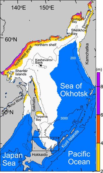
This update is to note a dramatic effect on Okhotsk Sea ice coincidental with the Polar Vortex event that froze Texas and other midwestern US states. When Arctic air extends so far south due to the weak and wavy vortex, warmer air replaces the icy air in Arctic regions. In this case, the deficits to sea ice extent appear mostly in the Sea of Okhotsk in the Pacific.
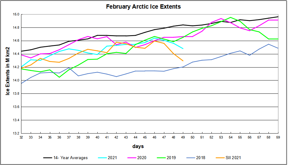
The graph below shows a sharp drop in ice extent the last three days.
A closer look into the regions shows that Okhotsk peaked at 1.1M km2 on day 37, and lost 217k km2 down to 0.9M km2 yesterday. That loss along with Bering flat extent makes up 70% of the present deficit to average.
Some comments from Dr. Judah Cohen Feb. 15 from his AER blog Arctic Oscillation and Polar Vortex Analysis and Forecasts Excerpts in italics with my bolds.
I have been writing how the stratospheric PV disruption that has been so influential on our weather since mid-January has been unusual and perhaps even unique in the observational record, so I guess then it should be no surprise that it’s ending is also highly unusual. I was admittedly skeptical, but it does seem that the coupling between the stratospheric PV and the tropospheric circulation is about to come to an abrupt end.
The elevated polar cap geopotential height anomalies (PCHs) related to what I like to refer to the third and final PV disruption at the end of January/early February quickly propagates to the surface and even amplifies, peaking this past weekend. And as I have argued, it is during spikes in PCH when severe winter is most likely across the NH mid-latitudes, as demonstrated in Cohen et al. (2018).
But rather than the typical gradual influence from the stratospheric PV disruption over many weeks, maybe akin to the drip, drip, drip of a leaky faucet, the entire signal dropped all at once like an anchor. This also likely contributed to the severity of the current Arctic outbreak in the Central US that is generational and even historical in its severity. But based on the forecast the PV gave all it had all at once, and the entire troposphere-stratosphere-troposphere coupling depicted in Figure ii is about to abruptly end in the next few days.
I am hesitant to bring analogs before 2000 but the extreme cold in Texas did remind me of another winter that brought historic Arctic outbreaks including cold to Texas – January 1977. It does appear that the downward influence from the stratospheric PV to the surface came to an abrupt end at the end of January 1977 . . . Relative to normal, January 1977 was the coldest month for both Eurasia and the US when stratosphere-troposphere coupling was active. But the relative cold did persist in both the Eastern US and northern Eurasia in February post the stratosphere-troposphere coupling. By March the cold weather in the Eastern US was over but persisted for northern Eurasia.
See also No, CO2 Doesn’t Drive the Polar Vortex
Background from Previous Post
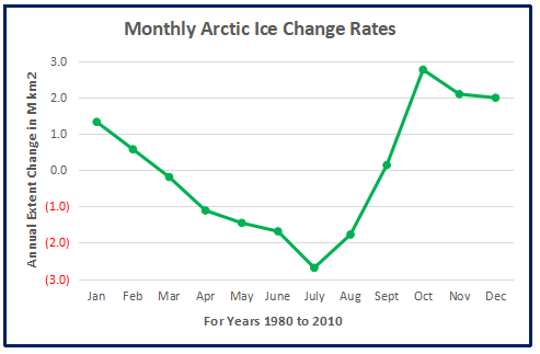
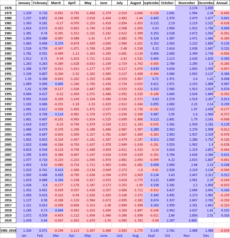
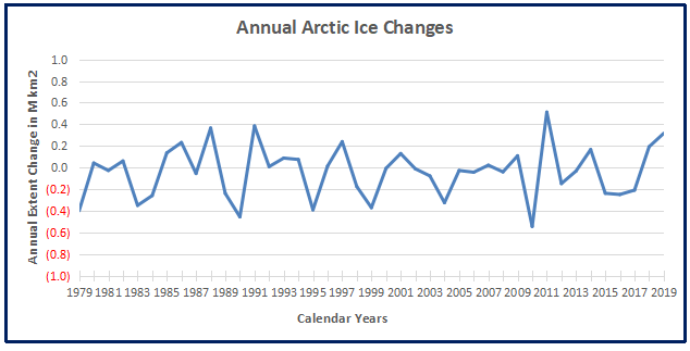
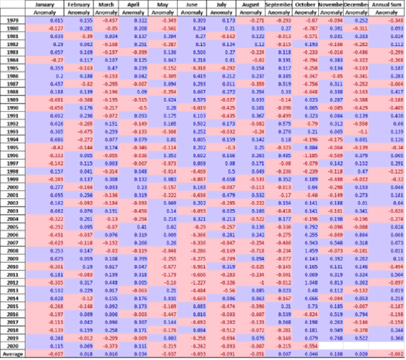
In January, most of the Arctic ocean basins are frozen over, and so the growth of ice extent slows down. According to SII (Sea Ice Index) January on average adds 1.3M km2, and this month it was 1.4M. (background is at Arctic Ice Year-End 2020). The few basins that can grow ice this time of year tend to fluctuate and alternate waxing and waning, which appears as a see saw pattern in these images.
Two weeks into February Arctic ice extents are growing faster than the 14-year average, such that they are approaching the mean. The graph below shows the ice recovery since mid-January for 2021, the 14-year average and several recent years.
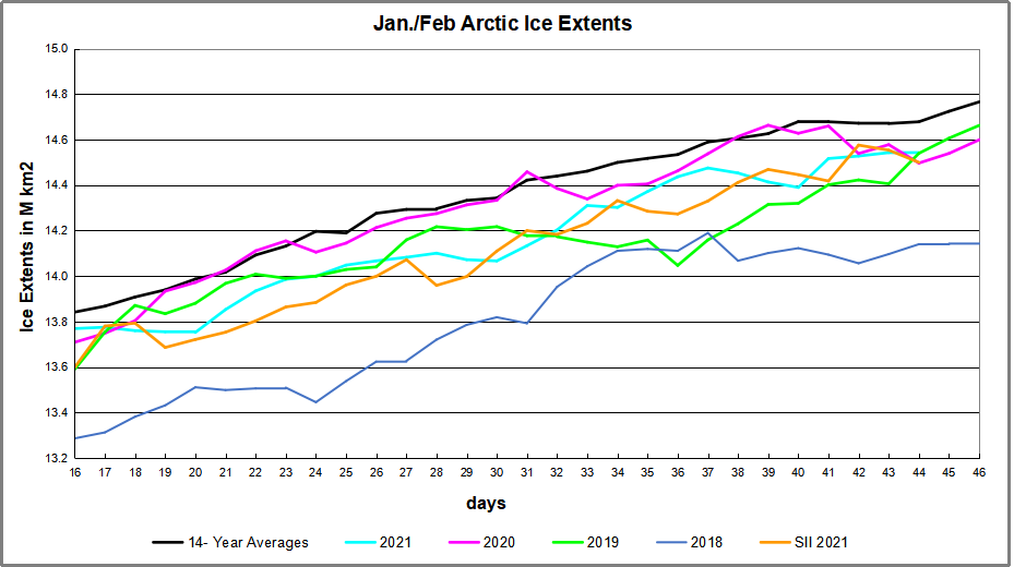
The graph shows mid January a small deficit to average, then slow 2021 growth for some days before picking up the pace in the latter weeks. Presently extents are slightly (1%) below average, close to 2019 and 2020 and higher than 2018.
February Ice Growth Despite See Saws in Atlantic and Pacific
As noted above, this time of year the Arctic adds ice on the fringes since the central basins are already frozen over. The animation above shows Barents Sea on the right (Atlantic side) grew in the last two weeks by 175k km2 and is now 9% greater than the maximum last March. Meanwhile on the left (Pacific side) Bering below and Okhotsk above wax and wane over this period. Okhotsk is seen growing 210k km2 the first week, and giving half of it back the second week. Bering waffles up and down ending sightly higher in the end.

The table below presents ice extents in the Arctic regions for day 44 (Feb. 13) compared to the 14 year average and 2018.
| Region | 2021044 | Day 044 Average | 2021-Ave. | 2018044 | 2021-2018 |
| (0) Northern_Hemisphere | 14546503 | 14678564 | -132061 | 14140166 | 406337 |
| (1) Beaufort_Sea | 1070689 | 1070254 | 435 | 1070445 | 244 |
| (2) Chukchi_Sea | 966006 | 965691 | 315 | 965971 | 35 |
| (3) East_Siberian_Sea | 1087120 | 1087134 | -14 | 1087120 | 0 |
| (4) Laptev_Sea | 897827 | 897842 | -15 | 897845 | -18 |
| (5) Kara_Sea | 934988 | 906346 | 28642 | 874714 | 60274 |
| (6) Barents_Sea | 837458 | 563224 | 274235 | 465024 | 372434 |
| (7) Greenland_Sea | 645918 | 610436 | 35482 | 529094 | 116824 |
| (8) Baffin_Bay_Gulf_of_St._Lawrence | 1057623 | 1487547 | -429924 | 1655681 | -598058 |
| (9) Canadian_Archipelago | 854597 | 853146 | 1451 | 853109 | 1489 |
| (10) Hudson_Bay | 1260471 | 1260741 | -270 | 1260838 | -367 |
| (11) Central_Arctic | 3206263 | 3211892 | -5630 | 3117143 | 89120 |
| (12) Bering_Sea | 559961 | 674196 | -114235 | 319927 | 240034 |
| (13) Baltic_Sea | 116090 | 94341 | 21749 | 76404 | 39686 |
| (14) Sea_of_Okhotsk | 1027249 | 930357 | 96892 | 911105 | 116144 |
| (15) Yellow_Sea | 9235 | 28237 | -19002 | 33313 | -24078 |
| (16) Cook_Inlet | 223 | 11137 | -10914 | 11029 | -10806 |
The table shows that Bering defict to average is offset by surplus in Okhotsk. Baffin Bay show the largest deficit, mostly offset by surpluses in Barents, Kara and Greenland Sea.
The polar bears have a Valentine Day’s wish for Arctic Ice.

And Arctic Ice loves them back, returning every year so the bears can roam and hunt for seals.

Footnote:
Seesaw accurately describes Arctic ice in another sense: The ice we see now is not the same ice we saw previously. It is better to think of the Arctic as an ice blender than as an ice cap, explained in the post The Great Arctic Ice Exchange.