Arctic Sea Ice | Science Matters

How About That Blob? (June 13 Update)

Posted on June 13, 2015 by Ron Clutz

June 13, 2015

As hoped for by Paris COP promoters, and by Californians looking for El Nino precipitation, the Blob in the North Pacific has intensified and may at least partly fulfill both expectations.

HADSST3 results for May are now in, and the sea surface temperature warming anomaly is up:

Global +0.12C over last May,
NH +0.16C over last May.

That will show up also in air temperature estimates, since 71% of the earth’s surface is covered by oceans. For example, UAH TLT anomalies show Global oceans +0.06C over last May, but Global land -0.1C, so Global UAH is only up +0.02C over May 2014. (Note: UAH uses satellites to measure air temperatures many meters above land or ocean, while surface datasets like HADCRUT, BEST, GISTEMP use the measured SSTs in their global mean temperature estimates).

The Blob difference shows up in UAH in the NH results: NH anomaly is +0.07 over last year, with the same increase showing over land and ocean. Interestingly, UAH shows the North Pole cooler than a year ago, the TLT over the Arctic being -0.06 less than a year ago. The South Pole land air temps are a whopping -0.2C colder than last May.

As far as Arctic Ice is concerned, the Blob probably caused the Bering Sea to melt out more than one month earlier than last year. About 10% of the water entering the Arctic Ocean comes from Bering, so there should be some impact on ice melting the immediate BCE region (Beaufort, Chukchi, East Siberian Seas). So far, in that region, 2015 is tracking last year’s melt at a slightly lower extent -4%, not yet a significant effect from the Blob.

Spitsbergen Triangle: Ground Zero for Climate Mysteries

Posted on June 8, 2015 by Ron Clutz

Credit to Dr. Bernaerts for his writings on this subject, excerpts of which appear below.

The Island Nexus for Ocean Currents

From the Dutch: spits – pointed, bergen – mountains

The largest and only permanently populated island of the Svalbard archipelago in northern Norway. Constituting the westernmost bulk of the archipelago, it borders the Arctic Ocean, the Norwegian Sea, and the Greenland Sea. Spitsbergen covers an area of 39,044 km2 (15,075 sq mi), making it the largest island in Norway and the 36th-largest in the world.

The fact is that the winter temperatures made a jump of more than eight degrees Celsius at the gate of the Arctic Basin, after 1918. Nowadays, one century later, the event is still regarded as “one of the most puzzling climate anomalies of the 20th century”.

Dr. Bernaerts:

The overriding aspect of the location is the sea; the sea around Spitsbergen, the sea between particularly the Norwegian, the Greenland, and the Barents Seas (Nordic Sea). The Norwegian Sea is a huge, 3000 metres deep basin. This huge water mass stores a great amount of energy, which can transfer warmth into the atmosphere for a long time. In contrast the Barents Sea, in the southeast of Spitsbergen has an average depth of just around 230 metres. In- and outflow are so high that the whole water body is completely renewed in less than 5 years. However, both sea areas are strongly influenced by the water masses coming from the South. The most important element is a separate branch of the North Atlantic Gulf Current, which brings very warm and very salty water into the Norwegian Sea and into the Spitsbergen region. Water temperature and degree of saltiness play a decisive role in the internal dynamics of the sea body. And what might be the role of the huge basin of the Arctic Ocean, 3000 meters depth and a size of about 15 million square kilometers?

The difference towards the other seas mentioned is tremendous. The Arctic Ocean used to be widely ice covered in the first half of the 20th Century, the other seas only partly on a seasonal basis. Only between the open sea and the atmosphere an intensive heat transfer is permanently taking place. Compact sea ice reduces this transfer about 90% and more, broken or floating ice may change the proportion marginally. In this respect an ice covered Arctic Ocean has not an oceanic but ‘continental’ impact on the climate.

The Arctic Ocean is permanently supplied with new water from the Gulf Current, which enters the sea close at the surface near Spitsbergen. This current is called the West Spitsbergen current. The arriving water is relatively warm (6 to 8°C) and salty (35.1 to 35.3%) and has a mean speed of ca. 30 cm/sec-1. The warm Atlantic water represents almost 90% of all water masses the Arctic receives. The other ~10% comes via the Bering Strait or rivers. Due to the fact that the warm Atlantic water reaches usually the edge of the Arctic Ocean at Spitsbergen in open water, the cooling process starts well before entering the Polar Sea.

A further highly significant climate aspect of global dimension is the water masses the Arctic releases back to oceans. Actually, the outflow occurs mainly via the Fram Strait between Northeast Greenland and Spitsbergen, and together with very cold water from the Norwegian Sea basin the deep water spreads below the permanent thermocline into the three oceans.

http://www.arctic-heats-up.com/pdf/chapter_2.pdf

The Spitsbergen Event 1918-1919

Beginning around 1850 the Little Ice Age ended and the climate began warming. Before that, at least since 1650 marked the first climatic minimum after a Medieval warm period, the Little Ice Age brought bitterly cold winters to many parts of the world, most thoroughly documented in the Northern Hemisphere in Europe and North America. The decreased solar activity and the increased volcanic activity are considered as causes. However, the temperature increase was remote and once again effected by the last major volcanic eruption of the Krakatoa in 1883. Up to the 1910s the warming of the world was modest.

Suddenly that changed. In the Arctic the temperatures literally exploded in winter 1918/19. The extraordinary event lasted from 1918 to 1939 is clearly demonstrated in the graph showing the ‘Arctic Annual Mean Temperature Anomalies 1880 – 2004’. But this extraordinary event has a number of facets, which could have been researched and explained. Meanwhile almost a full century has passed, and what do we know about this event today? Very little!

Studies considering the causation of the warming offer sketchy rather than well founded ideas. Here are a few examples:
• Natural variability is the most likely cause (Bengtsson, 2004);
• We theorize that the Arctic warming in the 1920s/1930s was due to natural fluctuations internal to the climate system (Johannessen, 2004).
• The low Arctic temperatures before 1920 had been caused by volcanic aerosol loading and solar radiation, but since 1920 increasing greenhouse gas concentration dominated the temperatures (Overpeck, 1997).
• The earlier warming shows large region-to-region, month-to-month, and year-to-year variability, which suggests that these composite temperature anomalies are due primarily to natural variability in weather systems (Overland, 2004).
• A combination of a global warming signal and fortuitous phasing of intrinsic climate patterns (Overland, 2008).

Arctic Regime Change

These explanations (and others such as CO2 or the AMOC) do not come to grips with how extreme and abrupt was this event. In the Spring of 1917, sea ice reached all the way to Spitsbergen, the only time in a century.

And the next year, temperatures rocketed upward, as shown by the weather station there:

A look at the SST history shows clearly an event as dramatic as a super El Nino causing a regime change. But this is the Atlantic, not the Pacific. Cooling followed, but temperatures stayed at a higher level than before.

Summary

The warming at Spitsbergen is one of the most outstanding climatic events since the volcanic eruption of Krakatoa, in 1883. The dramatic warming at Spitsbergen may hold key aspects for understanding how climate ticks. The following elaboration intends to approach the matter from different angles, but on a straight line of thoughts, namely:

WHERE: the warming was caused and sustained by the northern part of the Nordic Sea in the sea area of West Spitsbergen the pass way of the Spitsbergen Current.
WHEN: The date of the commencement of warming can be established with high precision of few months, and which was definitely in place by January 1919.
WHY: the sudden and significant temperature deviation around the winter of 1918/19 was with considerable probability caused, at least partly, by a devastating naval war which took place around the British Isles, between 1914 and 1918.

There is much more evidence and analysis supporting Dr. Bernaerts’ conclusions here:

http://climate-ocean.com/arctic-book/index.html

Conclusion: Unless your theory of climate change can make sense of the Spitsbergen Event, then it cannot inspire confidence. You may not be entirely convinced by Dr. Bernaerts’ explanation, but he at least has one–nobody else has even tried.

Climate on Ice: Ocean-Ice Dynamics

Posted on May 26, 2015 by Ron Clutz

Update May 30, 2015 Longer term context by E.M. Smith added below

Sea ice is not simple. Some Background is in order.

When white men started to explore the north of America, they first encountered the Crees. Hudson Bay posts were established to trade goods for pelts, especially the beavers used for making those top hats worn by every gentleman of the day.

The Crees told the whites that further on toward the Arctic Circle there were others they called “eskimos”. The Cree word means “eaters of raw meat” and it is derogatory. The Inuit (as they call themselves) were found to have dozens of words for snow, a necessary vocabulary for surviving in the Arctic world.

A recent lexicon of sea ice terminology in Nunavik (Appendix A of the collective work Siku: Knowing our Ice, 2008) comprises no fewer than 93 different words. These include general appellations such as siku, but also terms as specialized as qautsaulittuq, ice that breaks after its strength has been tested with a harpoon; kiviniq, a depression in shore ice caused by the weight of the water that passed over and accumulated on its surface during the tide; or iniruvik, ice that cracked because of tide changes and that the cold weather refroze.

http://www.thecanadianencyclopedia.ca/en/article/inuit-words-for-snow-and-ice/

With such complexity of ice conditions, we must recognize that any general understanding of ocean-ice dynamics will not be descriptive of all micro-scale effects on local or regional circumstances.

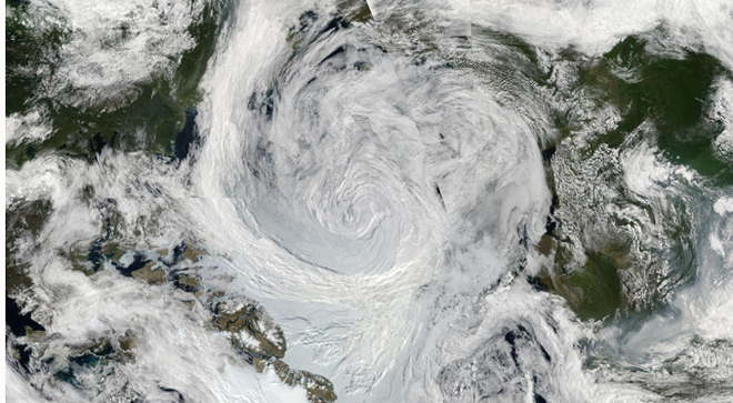
Short Term Sea Ice Freezing and Melting Cycle

Alarmists only mention positive feedbacks from ice melting, so one is left to wonder why there is any Arctic ice left so many years since the Little Ice Age ended around 1850. Actually there are both positive and negative feedbacks, with one or the other dominating at different times and places.

Of course, the basic cycle is the seasonality of sunless winters and sunlit summers.

Remember that ice grows because of a transfer of heat from the relatively warm ocean to the cold air above. Also remember that ice insulates the ocean from the atmosphere and inhibits this heat transfer. The amount of insulation depends on the thickness of the ice; thicker ice allows less heat transfer. If the ice becomes thick enough that no heat from the ocean can be conducted through the ice, then ice stops growing. This is called the thermodynamic equilibrium thickness. It may take several years of growth and melt for ice to reach the equilibrium thickness. In the Arctic, the thermodynamic equilibrium thickness of sea ice is approximately 3 meters (9 feet). However, dynamics can yield sea ice thicknesses of 10 meters (30 feet) or more. Equilibrium thickness of sea ice is much lower in Antarctica, typically ranging from 1 to 2 meters (3 to 6 feet).

Snow has an even higher albedo than sea ice, and so thick sea ice covered with snow reflects as much as 90 percent of the incoming solar radiation. This serves to insulate the sea ice, maintaining cold temperatures and delaying ice melt in the summer. After the snow does begin to melt, and because shallow melt ponds have an albedo of approximately 0.2 to 0.4, the surface albedo drops to about 0.75. As melt ponds grow and deepen, the surface albedo can drop to 0.15. As a result, melt ponds are associated with higher energy absorption and a more rapid ice melt.

https://nsidc.org/cryosphere/seaice/processes/growth_melt_cycle.html

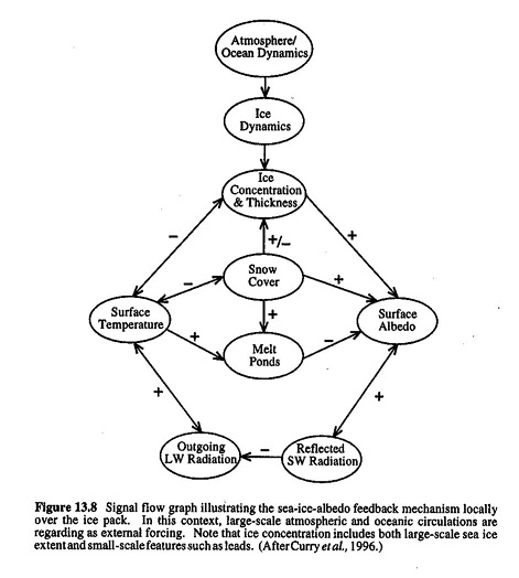
The short-term dynamics of sea ice freezing and melting can be summarized in this diagram from Dr. Judith Curry:

Dr. Curry has written extensively on sea ice, and an introduction to her sources is here:

http://judithcurry.com/2014/10/15/new-presentations-on-sea-ice/

Decadal Variability in Sea Ice Extent

Medium term sea ice variations are well described by Lawrence A. Mysak and Silvia A. Venegas of the Centre for Climate and Global Change Research and Department of Atmospheric and Oceanic
Sciences, McGill University, Montreal, Quebec, Canada.

Abstract: A combined complex empirical orthogonal function analysis of 40 years of annual sea ice concentration (SIC) and winter sea level pressure (SLP) data reveals the existence of an approximately 10-year climate cycle in the Arctic and subarctic.

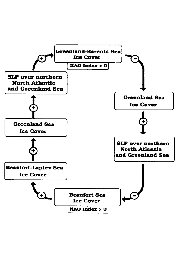
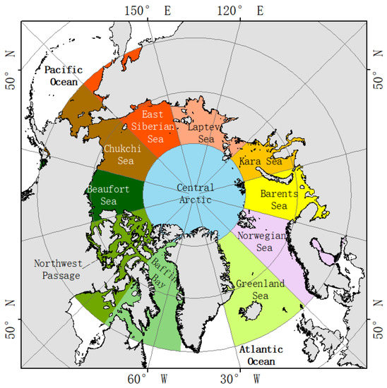
“Starting at the top of the loop in Figure 4, we propose that large SIC (Sea Ice Concentration) positive anomalies are created in the Greenland Sea by a combination of anomalous northerly winds and a relatively small northward transport of warm air (sensible heat) [Higuchi et al., 1991] associated with a negative NAO pattern. The relationship between severe sea ice conditions in the Greenland Sea and a weak atmospheric circulation (negative NAO) was previously noticed by Power and Mysak [1992]. Over the Barents Sea, on the other hand, the formation of the large positive SIC anomalies may be mainly due to weaker-than-normal advection of warm water by the northward branch of the North Atlantic Current when the NAO index is negative (R. R. Dickson, pets.comm., 1998).”

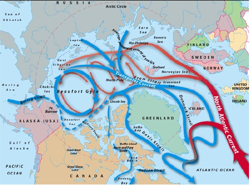
“These SIC anomalies are then advected into the Labrador Sea by the local mean ocean circulation over a 3-4 year period. When the southern part of the Greenland Sea thus becomes relatively ice free (as implied by the minus sign at the upper-right corner of the loop), strong heating of the atmosphere during winter occurs, which is hypothesized to cause the Icelandic Low to deepen at that time (hence the plus sign on the right-hand side of the loop). This may help change the polarity of the NAO. When the NAO index is positive (deep Icelandic Low), the wind anomalies create positive SIC anomalies in the Beaufort Sea (see bottom of the loop), which are then slowly advected out of the Arctic via the Beaufort Gyre and Transpolar Drift Stream over a 3-4 year period (see lower-left corner and left-hand side of loop).”

“As a consequence, the Greenland Sea becomes extensively ice covered, which suddenly cuts off the heat flux to the atmosphere during winter and hence is likely to cause the Icelandic Low to weaken at that time, which may contribute to changing the NAO polarity. This brings us back to the beginning of the cycle (top of Figure 4) after about 10 years.”

Click to access paper_ice_Mysak1998.pdf

Multi-Decadal Sea Ice Dynamics

In a 2005 publication Mysak presents additional empirical evidence for these ocean-ice mechanisms:

“In this paper we have shown that an intermediate complexity climate model consisting of a 3-D ocean component, a state-of-the-art sea-ice model (with elastic-viscous-plastic rheology) and an atmospheric energy-moisture balance model can successfully simulate a large number of observed changes in the Arctic Ocean and sea-ice cover during the past half-century.”

“Morison et al. (1998) found an increase in both the temperature and salinity at depths of 200–300 m in the eastern Arctic. . .This increase in salinity is also supported by the work of Steele and Boyd (1998) who found that the winter mixed layer in the Eurasian Basin had higher salinity values in the early 1990s compared with the 40-year record of the Environmental Working Group (EWG) Joint US-Russian Arctic Atlas. Morison et al. (1998) argue that the increase in salinity represents a westward advance into the Arctic of the front between the waters of the eastern and western Arctic. The aforementioned temperature and salinity changes support the hypothesis that the warm and salty Atlantic water penetrated further into the central Arctic Basin during the 1990s, and thus has pushed the front between Atlantic derived and Pacific derived waters westward.”

Click to access Mysak_et_al_2005.pdf

Summary: Sea Ice Impacts Climate Strongly, this century and beyond.

“Sea ice is a key player in the climate system, affecting local, and to some degree remote regions, via its albedo effect. Sea ice also strongly reduces air-sea heat and moisture fluxes (Ruddiman and McIntyre 1981; Gildor and Tziperman 2000), and thus may cause the air overlying it to be cooler and drier compare to air overlying ice-free ocean (Chiang and Bitz 2005). A significant part (*33 %) of the precipitation over the northern hemisphere (NH) ice sheets is believed to have originated locally from the Norwegian, Greenland and the Arctic seas (Charles et al. 1994;Colleoni et al. 2011). Lastly, sea ice affects the location of the storm track and therefore indirectly also the patterns of precipitation (e.g. Laine et al. 2009; Li and Battisti 2008).”

“Its effect on the hydrological cycle makes sea ice a potentially significant player in the temperature-precipitation feedback (Le-Treut and Ghil 1983), according to which increase in temperature intensifies the hydrological cycle and thus the snow accumulation over ice sheets. This feedback is an important part of the sea-ice switch mechanism for glacial cycles, for example Gildor and Tziperman (2000). Indeed, proxy records show drastic increase in accumulation rate during interstadial periods (Cuffey and Clow 1997; Alley et al. 1993; Lorius et al. 1979), when the sea-ice retreats from its maximal extent.”

The largest ice cap in the Eurasian Arctic – Austfonna in Svalbard – is 150 miles long with a thousand waterfalls in the summer

“We find that in a cold, glacial climate snowfall rate over the ice sheets is reduced as a result of increasing sea-ice extent (compare LGM and PDSI experiments). An increased sea-ice extent cools the climate even more, the precipitation belt is pushed southward and the hydrological cycle weakens.

We find that the albedo feedback of an extended sea-ice cover in an LGM-like climate only weakly affects the reduction of snowfall rate.

indicating that the insulating feedback is responsible for a large part of the suppression of precipitation by sea ice. It follows that the hydrological cycle is more sensitive to the insulating effect of sea ice than to its albedo. There are two reasons to the larger contribution of the insulating effect to the temperature-precipitation feedback. First, the overall cooling of the insulating effect is about twice than that of the albedo. This by itself is expected to lead to a more significant change in precipitation. In addition, the insulation effect not only reduce air-sea heat flux, it also directly prevents evaporation from ice-covered regions, which are a major source of precipitation over the NH ice sheets (Charles et al. 1994).

Click to access tziperman_sea.pdf

Conclusion: It’s the Ice and the Water

Regardless of the uncertainties in the underlying principal mechanisms of the sea ice-AMO-AMOC linkages, it is clear that multidecadal sea-ice variability is directly or indirectly related to natural fluctuations in the North Atlantic. This study provides strong, long-term evidence to support modeling results that have suggested linkages between Arctic sea ice and Atlantic multidecadal variability [Holland et al., 2001; Jungclaus et al., 2005; Mahajan et al., 2011].

Here we present observational evidence for pervasive and persistent multidecadal sea ice variability, based on time-frequency analysis of a comprehensive set of several long historical and paleoproxy sea ice records from multiple regions. Moreover, through explicit comparisons with instrumental and proxy records, we demonstrate covariability with the Atlantic Multidecadal Oscillation (AMO).

Click to access Gildor-Ashkenazy-Tziperman-Lev-2014.pdf

Update May 30,2015 From E.M. Smith and Salvatore Del Prete

I think I can take a crack as answering some of the questions and pointing at a likely structure for some of the other bits.

Why is it whenever the climate changes the climate does not stray indefinitely from it’s mean in either a positive or negative direction? Why or rather what ALWAYS brings the climate back toward it’s mean value ? Why does the climate never go in the same direction once it heads in that direction?

IMHO the answer is that there is a hysteresis from water that limits the excursions. On one end, freezing tends to cut down heat dumping as frozen ice does not radiate as much heat to space. On the other end, tropical storm formation limits heat in the equatorial oceans as you get more water evaporation / rise / precipitation cycles and more radiation to space from the tropopause / stratosphere. So we don’t get ‘brought back to the mean’, but rather switch from an ice ball (most of the time) to a warm & wet (10% of the time). This switching is the Malankovitch cycle, and it is driven by changes in the orbital roundness, precession of the equinox, and changes of tilt of the planet (that are not really changes of tilt, they are changes in position relative to the celestial equator.

Much more here:

https://chiefio.wordpress.com/2015/05/29/salvatore-del-prete-thesis/

Okhotsk, Barents, Who Cares?

Posted on April 18, 2015 by Ron Clutz

More people are familiar with the above brand of work and casual wear than know of the similarly named sea near the Arctic Circle. And many confuse the Barents and Bering Seas which are on opposite sides of the Arctic. So what?

Here’s the thing: This year’s NH sea ice extent (Arctic plus nearby seas) is down. And so we’re getting the warnings about the Arctic “death spiral” and starving polar bears. It turns out that most of the difference between this year and last comes from less ice in Okhotsk and Barents.

So it is very timely that Dr. Bernaerts has posted an essay on events shaping the climate in those two places:
Arctic sea ice record low – 02/25/2015
and human offshore activities not to blame – at least a bit?
http://www.ocean-climate-law.com/13/Arch/5.html

While the total maximum ice extent in NH is always 14-16 MKm2, both OKhotsk and Barents max extents vary a lot year to year. For example, the Sea of Okhotsk covers 1.58 MKm2 – it’s a huge basin that was virtually filled with ice in March 1979 but only about 1/3 filled in 2015.

Both seas cover about the same area (1,5 Mio. km²), the Sea of Okhotsk with an average depth of 859 m, and the Barents Sea only 230 m, but differ grossly in many other aspects. While the latter is a continental Shelf, with three islands (Spitsbergen, Franz Josef Land and Novaya Zemlya) as boundaries and open to the North Atlantic and Arctic Ocean, the Sea of Okhotsk is semi enclosed, with an internal current system (Fig. 8-9).

Okhotsk will lose all its ice by July, and Barents usually retains less than 20%.

Bernaerts’ larger point is that in addition to natural variations in circulations, winds and clouds, human activity is also changing the climate, and particularly the ice extent in these places. Both have extensive fishing and commercial shipping, ice-breakers operating, submarine fleet exercises, sea bottom oil extraction, etc. All of these have an effect in the direction of inhibiting ice formation.

Oh, and about the polar bears: They have never been at Okhotsk and never will be. As for Barents, the ice conditions are providing suitable hunting conditions for the polar bears (perhaps the seals deserve a warning).
http://polarbearscience.com/2015/04/12/challenging-polar-bear-fearmongering-about-arctic-sea-ice-extent-for-march-2015/

Dr. Bernaerts concludes:

“The recent new Arctic sea ice record gives little reason for lamenting, but should be seen as an opportunity to investigate and understand the human activities in the Barents and Okhotsk Sea. It could be observed that both seas differed most from average due to warmer sea water temperature. Although it may be difficult to assess the impact of worldwide shipping and fishing on climatic changes and ‘global warming’, it is a much lower challenge if only the impact of two regional seas, representing only about 1% of the global water surface, is investigated.”
http://www.ocean-climate-law.com/13/Arch/5.html

Heraclitus (535 BC – 475 BC) famously said, “No man ever steps in the same river twice.” The same can be said for anyone sailing in these seas.

Footnote:
After the early arrival at maximum in February, NH ice extent went sideways and is now on the track of recent years. Where it goes from here is always entertaining.

Analysis of NOAA Arctic Sea Ice extent since 1979

Posted on March 31, 2015 by Ron Clutz

For climate analysis we consider the average monthly extents for March and for September of each year in the satellite record, and the differences (the melt extent). Though we would prefer a longer record, these are currently the most popular data. Several observations:

March averages (annual maximums) do not vary greatly: 15.48 M Km2 is the average extent, with a range of 16.45 to 14.43 M Km2. 2/3 of the years are between 15 and 16M.

September averages (annual minimums) vary much more: 6.40 M Km2 is the average, with a range of 7.88 to 3.63 M Km2. Standard deviation is +/- 1.07 M Km2.

Note: The largest September extent (7.88) in the record occurred in 1996, the same year of the smallest melt extent: 7.25. And the smallest September extent (3.63) occurred in 2012, due to the largest melt in the record, 11.8M. The March extents of those two years were nearly the same.

The Arctic ice extent time series appears to consist of three periods:
1979 to 1996 Annual minimums mostly above average
1997 to 2006 Annual minimums around average
2007 to 2014 Annual minimums below average

Averages	March	Sept	Diff (Melt)
1979 to 1996	15.8	7.2	8.6
1997 to 2006	15.3	6.2	9.0
2007 to 2014	15.0	4.5	10.5

Since 2005 the combination of below average March extents, combined with above average melts has produced September extents below 6 M Km2 each year.

It is now evident that 2012 was an outlier (probably due to the unusual storm activity). That year’s melt of 11.8 was 28% above the average melt of 9.09 and more than 1 M km2 larger than the second largest melt in 2008.

The pivotal decade was 1997 to 2006, preceded by slightly declining extents, and followed by much lower extents. What any of this has to do with CO2 and air temperatures is not obvious.

Data is here:
ftp://sidads.colorado.edu/DATASETS/NOAA/G02135/Mar/N_03_area.txt
ftp://sidads.colorado.edu/DATASETS/NOAA/G02135/Sep/N_09_area.txt

Comparing NOAA to MASIE Arctic Ice Extent

Posted on March 31, 2015 by Ron Clutz

Some might be interested to compare MASIE results with NOAA Sea Ice Index, since NOAA is a typical reference for Arctic Ice news. NOAA uses only passive microwave readings, while MASIE includes other sources, such as satellite images and field observations.

For comparison, MASIE shows about 700,000 Km2 more ice extent than NOAA both at maximum and minimum. This is usually explained by microwave sensors seeing melt water on top of ice the same as open water.

For the years 2007 to 2014 inclusive, each year MASIE shows higher maximums than NOAA, on average 5% higher. In each of those same years MASIE shows higher minimums than NOAA, on average 15% higher. The melt extent is more comparable: NOAA shows an average annual loss of 70.5 %, while MASIE shows an average loss of 67.5%.

NIC Ice Charts

Climatologists say the NIC estimates are “conservative.” By this they mean NIC’s priority is shipping safety, and so, when in doubt, under mixed ice and water conditions, ice charts show ice. NIC people do not make predictions about sea ice, they only report what is there, according to their multiple sources.

On the other hand, principals at both NASA and NOAA have said on the record that the Arctic will soon be ice-free, and it will be the fault of CO2. Could it be when in doubt, under mixed conditions, they report water in places where NIC shows ice? That would explain the discrepancies in estimates of ice extent

Note: NOAA has bureaucratic authority over NIC and advises against using NIC records for climate analysis. Last year, NIC results became available only on a rolling 30-day basis, so that estimates older than the current period are no longer available. Noticing this policy change, I began building a spreadsheet to capture the history for my own analysis. Since mid November, 2014, NIC ice extent reports have been unavailable at the MASIE webpage.

Update on April 2: NSIDC now says MASIE will be back after April.

Update November 2015: MASIE dataset is now available from January 1, 2006 to the present.

Everything You Wanted to Know about Measuring Arctic Ice (But Were Afraid to Ask)

Posted on March 30, 2015 by Ron Clutz

There are several research centers that monitor Arctic ice extent, especially NSIDC (USA), DMI (Denmark), JAXA (Japan), and NANSEN (Norway). All start with the same data from passive microwave sensors on NASA satellites. Slight differences arise from different algorithms used to process the inputs into ice extent estimates.

Operational ice charts are an alternative measure of Arctic sea ice extent. These are prepared daily by Canada, Russia and US maritime authorities to assist ships navigating in Arctic waters. For example, the US National Ice Center (NIC) provides an index called MASIE (Multisensor Analyzed Sea Ice Extent). NIC charts are based upon not only passive microwave numbers, but also satellite imagery and reports from planes and ships operating in the regions. Operational ice charts are the most detailed pre-satellite records, with the Russian archives being the oldest.

What’s the Issue?

On another blog, a climate person put it to me this way:

“Based on what I’ve read if I had no other source, or were heading out in a boat, I would most certainly use the operational indices such as NIC. For climate change trends, I’d go with NSIDC, JAXA … Do you know of any climate scientists that prefer NIC?”

Measuring anything in the Arctic is problematic due to the conditions. And any technology has limitations and uncertainties. Thus it is useful to have more than one estimate of ice extent. Comparisons of the two types of data show the passive microwave results underestimate ice extent, especially during the late summer minimum. The difficulty is mistaking surface melt water for open water, failing to discern the ice underneath.

“Passive microwave sensors from the U.S. Defense Meteorological Satellite Program have long provided a key source of information on Arctic-wide sea ice conditions, but suffer from some known deficiencies, notably a tendency to underestimate ice concentrations in summer. With the recent release of digital and quality controlled ice charts extending back to 1972 from the U.S. National Ice Center (NIC), there is now an alternative record of late twentieth century Northern Hemisphere sea ice conditions to compare with the valuable, but imperfect, passive microwave sea ice record.”

“This analysis has been based on ice chart data rather than the more commonly analyzed passive microwave derived ice concentrations. Differences between the NIC ice chart sea ice record and the passive microwave sea ice record are highly significant despite the fact that the NIC charts are semi-dependent on the passive microwave data, and it is worth noting these differences. We compare the ice chart data to ice concentrations from the NASA Team algorithm which, along with the Bootstrap algorithm [Comiso, 1995], has proved to be perhaps the most popular used for generating ice concentrations [Cavalieri et al.,1997]. We find a baseline difference in integrated ice concentration coverage north of 45N of 3.85% ± 0.73% during November to May (ice chart concentrations are larger). In summer, the difference between the two sources of data rises to a maximum of 23% peaking in early August, equivalent to ice coverage the size of Greenland.“ ( My Bold) Source: Late twentieth century Northern Hemisphere sea-ice record from U.S. National Ice Center ice charts.

The differences are even greater for Canadian regions.

“More than 1380 regional Canadian weekly sea-ice charts for four Canadian regions and 839 hemispheric U.S. weekly sea-ice charts from 1979 to 1996 are compared with passive microwave sea-ice concentration estimates using the National Aeronautics and Space Administration (NASA) Team algorithm. Compared with the Canadian regional ice charts, the NASA Team algorithm underestimates the total ice-covered area by 20.4% to 33.5% during ice melt in the summer and by 7.6% to 43.5% during ice growth in the late fall.”

From: The Use of Operational Ice Charts for Evaluating Passive Microwave Ice Concentration Data, Agnew and Howell

Or, if you don’t like what the US or Canada puts in their ice charts, you can get a third, independent perspective from Russia. The AARI has been studying and mapping the polar regions for a very long time, currently one of them chairs the ETSI and they maintain a global sea ice database (the other one is at NSIDC). Their ice charts can be accessed here.

A warning note: The Russians are not alarmed by what they see in the Arctic.

“In winter, the newly formed ice actively grows up to a 1.2 meter thick layer, while the coastal ice grows up to 2.0 meters. Consequently, the Arctic sea ice layer does not change significantly. Moreover, according to Genrikh Alekseev, in the summer, ice melts in various seas unequally. This year, the seas through which the Northern Shipping Route passes are covered with an unusually thicker ice layer. The Barents Sea is covered by a thin ice layer, but the amount of ice in the Kara, Laptev, East-Siberian and Chukotskiy seas exceeds the level of 2007. The conditions in the Arctic in the warm summer can be considered abnormal, but the Northern Shipping Route has not been completely freed from ice yet. This means icebreakers will be needed in the future, says the scientist.”

The extreme melting of ice in the summer 2012 is most likely the last gesture that the warming is ending. In fact, ice is a product of climate, and when comparing the graphs of the air temperature and melting ice, one can see that they coincide, Genrikh Alekseev said.

Conclusion:

Operational ice charts are more variable due to human error in their production.

Climatologists prefer passive microwave indices of ice extent because they are consistently wrong.

One wonders about their preference if satellites were overestimating ice. For myself I am glad for two mostly independent measures, one done by people who only want to get it right that day.

Note: As of March 2015, NSIDC has been showing MASIE off-line since mid November 2014. They say NIC results will be back in April.

Update on April 2: NSIDC now says MASIE will be back after April.

Arctic Sea Ice Factors

Posted on March 29, 2015 by Ron Clutz

An early-spring sunset over the icy Chukchi Sea near Barrow (Utqiaġvik), Alaska, documented during the OASIS field project (Ocean_Atmosphere_Sea Ice_Snowpack) on March 22, 2009. Image credit: UCAR, photo by Carlye Calvin.

Alarmists are always claiming the Arctic Sea Ice is the “canary in the coal mine.” Wrong. Arctic ice extent varies a lot for a lot of reasons. Predictions of its disappearing because of rising CO2 are another attempt to use a natural process as proof that global warming is dangerous and linked to fossil fuel emissions.

The Long View of NH Sea Ice

First some historical context for how NH ice extent varies over decades and centuries.

Figure 16-3: Time series of April sea-ice extent in Nordic Sea (1864-1998) given by 2-year running mean and second-order polynomial curves. Top: Nordic Sea; middle: eastern area; bottom: western area (after Vinje, 2000). IPCC Third Assessment Report

“The extent of ice in the Nordic Seas measured in April has been subject to a reduction of ~33% over the past 135 yr. Nearly half of this reduction is observed over the period ~1860–1900, prior to the warming of the Arctic. Decadal variations with an average period of 12–14 yr are observed for the whole period. The observation series indicates that less than 3% of the variance with respect to time can be explained for a series shorter than 30 yr, less than 18% for a series shorter than 90 yr, and less than 42% for the whole 135-yr long series. While the mean annual reduction of the April ice extent is decelerating by a factor of 3 between 1880 and 1980, the mean annual reduction of the August ice extent is proceeding linearly.”

“The August ice extent in the Eastern area has been more than halved over the past 80 yr. A similar meltback has not been observed since the temperature optimum during the eighteenth century. This retrospective comparison indicates accordingly that the recent reduction of the ice extent in the Eastern area is still within the variation range observed over the past 300 yr.”

Anomalies and Trends of Sea-Ice Extent and Atmospheric Circulation in the Nordic Seas during the Period 1864–1998 by TORGNY VINJE, Norwegian Polar Institute, Oslo, Norway

http://journals.ametsoc.org/doi/pdf/10.1175/1520-0442(2001)014%3C0255%3AAATOSI%3E2.0.CO%3B2

Multiple Factors Affecting Sea Ice Extent

The references below, among many others, show that the factors causing Arctic Ice to lessen, when that was happening, have nothing to do with air temperatures which is the only way CO2 could have an effect (theoretically). The melting is much more the result of water circulations, especially when warm Atlantic water from the south is able, or not, to get into the Arctic Ocean.

“Regional Arctic sea ice variations result from atmospheric circulation changes and in particular from ENSO and North Atlantic Oscillation (NAO) events. Patterns of Arctic surface air temperature changes and trends are consistent with regional changes in sea ice extent. A dominant mode of Arctic variability is the Arctic Oscillation (AO), and its strong positive phase during the 1990s may account for much of the recent decrease in Arctic ice extent. The AO explains more than half of the surface air temperature trends over much of the Arctic.”
http://onlinelibrary.wiley.com/enhanced/doi/10.1029/2003GL018031/

“The variation in the ice extent caused by a 1C change in the ocean temperature since 1860 compares with about 90% of the concurrent total ice extent variation observed in the eastern area. The net effect of atmospheric temperatures seems accordingly to be relatively small over the same period of time. This concurs with the large difference in the individual heat capacity.”

http://journals.ametsoc.org/doi/pdf/10.1175/1520-0442(2001)014%3C0255%3AAATOSI%3E2.0.CO%3B2

“So why does circulation matter? Two reasons. First off, you can see warm water entering on the Pacific and Atlantic connections and cold water leaving via Canada and Greenland / Fram Strait. During a Glacial, that circulation stops. With a mile of ice over Canada, that exit is closed. With ocean levels 100 meters lower, folks can walk from Russia to Alaska. (Well, they do it sometimes now over the ice, but it will be easier and less seasonal during a Glacial).”

“So look again. No Bering Sea warm intrusion. No Canadian cold drain. No Beaufort Gyre when the ice is deep, since there will be no wind driven circulation under the ice. The Asian current toward the Bering Sea will end. The entire Asian warm river drain into the Arctic likely freezes up and doesn’t happen – which raises the interesting question of where does it go then? But that is for another day. Like asking where the Alaskan rivers drain then, or are they just glaciers at that point?”

“In short, what is left is just the North Atlantic Drift (aka Gulf Stream for Americans) warming a small patch near Europe and some cold water near Greenland. As Scotland was under ice in the last Glacial, even that North Atlantic Drift circulation likely didn’t get very far north.”
https://chiefio.wordpress.com/2014/05/04/arctic-flushing-and-interglacial-melt-pulses/

In addition to water circulation effects, sea ice extent is influenced by clouds and winds.

“Researchers have found that the high amounts of cloud in the early summer lead to low concentrations of sea ice in the late summer. This relationship between cloud cover and sea ice is so strong that it can explain up to 80 per cent of the variation in sea ice over as much as 60 per cent of the the sea ice area.”

http://www.reportingclimatescience.com/news-stories/article/high-cloud-levels-drive-low-arctic-sea-ice.html

“We have shown evidence that low level winds over the Arctic, play an important role in mediating the rate of retreat of sea ice during summer. Anomalous anticyclonic flow over the interior of the Arctic directed toward the Fram Strait favors rapid retreat and vice versa. We have argued that the relative rankings of the September SIE for the years 2007, 2010 and 2011 are largely attributable to the differing rates of decrease of SIE during these summers, which are a consequence of year-to-year differences in the seasonal evolution of summertime winds over the Arctic. . . It is not clear why anticyclonic wind anomalies have been prevalent in recent years. ”

Click to access 2012GL051330.pdf

Conclusion:

Like most things in the climate, Arctic sea ice extent is determined by many interacting factors. Among those many influences, the weakest case is claiming CO2 as a driving force.

	HadCRUT5 temperature… on Yearend 2025, Cooling Temperat…
	HadCRUT5 temperature… on More Evidence Temperatures Dri…
	Slam Dunk: Δtemp Dri… on Yearend 2025, Cooling Temperat…
	Ron Clutz on December 2025 All Ocean SSTs C…
	oldbrew on December 2025 All Ocean SSTs C…