Tweak the Sun’s Rotation, and We’re Not Here

Watch the Sun rotate for over a month brought to you by SDO. Since the Sun rotates once every 27 days on average, this movie presents more than an entire solar rotation. From March 30 through Apr. 29, 2011, the Sun sported quite a few active regions and magnetic loops. The movie shows the Sun in the 171 Angstrom wavelength of extreme ultraviolet light (capturing ionized iron heated to about 600,000 degrees), color coded to appear gold. The movie is based on a frame taken every 15 minutes being shown at 24 frames per second, with very few data gaps in this almost two-minute movie. Source Solar Dynamics Observatory

Another fresh reminder we owe our existence to the sun along with the climate in which we evolved and adapted. The Forbes article is Early Sun’s ‘Goldilocks’ Rotation Rate May Be Why We’re Here  Excerpts in italics with my bolds.

Our early Sun’s rate of rotation may be one reason we’re here to talk about it, astrobiologists now say. The key likely lies in the fact that between the first hundred million to the first billion years of its life, our G-dwarf star likely had a ‘Goldilocks’ rotation rate; neither too slow nor too fast.

Instead, its hypothetical ‘intermediate’ few days rate of rotation guaranteed our Sun was active enough to rid our newly-formed Earth of its inhospitable, hydrogen-rich primary atmosphere. This would have enabled a more habitable, secondary atmosphere composed of nitrogen, carbon dioxide, hydrogen and oxygen to eventually form.

If it had been a ‘fast’ (less than one day rotator), our Sun might have continually stripped our young planet of its secondary atmosphere as well. However, if it took more than 10 days to rotate, it might not have been active enough to strip Earth of its hypothetical primary atmosphere.

Such ideas were recently bandied about in oral presentations at last month’s the General Assembly of the International Astronomical Union (IAU) in Vienna.

Earth’s very first atmosphere would have been too hot and too thick, more like Venus’ present-day atmosphere, Theresa Luftinger, an astrophysicist at the University of Vienna, told me. No known organisms could have evolved under such an atmosphere.  A secondary atmosphere cannot evolve in the presence of a primordial atmosphere , says Luftinger.

It’s the star’s magnetic dynamo that drives its magnetic fields. And these magnetic fields, in turn, interact with the star itself, creating an interplay of extreme stellar activity.

“So, the quicker the star rotates, the higher the interaction between the magnetic field and the stellar body ,” said Luftinger.

Faster rotation means higher extreme ultra-violet and x-ray activity, Helmut Lammer, an astrophysicist at Austria’s Space Science Institute in Graz, told me. This would lead to atmospheric stripping and water loss on earthlike planets around an active young star, he says. 

Our Sun is now a very slow rotator at 27 days. But that wasn’t always the case. As for why some stars seem to inherently rotate faster than others?

Astrophysicists suspect that initial conditions within star-forming clouds cause newborn stars to have different rotation rates.

Researchers are able to roughly pinpoint the Sun’s early rotation rates by studying the isotopic ratios of neon, argon, potassium, and uranium here in Earth’s crust. That is, elements which have atoms that have the same numbers of protons in their atomic nucleus, but different numbers of neutrons. The researchers also considered such isotopic ratios from decades’-old Venus surface samples taken by Soviet Venus lander missions.


Ocean Air Temps Tepid in July

Presently sea surface temperatures (SST) are the best available indicator of heat content gained or lost from earth’s climate system.  Enthalpy is the thermodynamic term for total heat content in a system, and humidity differences in air parcels affect enthalpy.  Measuring water temperature directly avoids distorted impressions from air measurements.  In addition, ocean covers 71% of the planet surface and thus dominates surface temperature estimates.  Eventually we will likely have reliable means of recording water temperatures at depth.

Recently, Dr. Ole Humlum reported from his research that air temperatures lag 2-3 months behind changes in SST.  He also observed that changes in CO2 atmospheric concentrations lag behind SST by 11-12 months.  This latter point is addressed in a previous post Who to Blame for Rising CO2?

The July update to HadSST3 will appear later this month, but in the meantime we can look at lower troposphere temperatures (TLT) from UAHv6 which are already posted for July. The temperature record is derived from microwave sounding units (MSU) on board satellites like the one pictured above.

The UAH dataset includes temperature results for air above the oceans, and thus should be most comparable to the SSTs. There is the additional feature that ocean air temps avoid Urban Heat Islands (UHI).  The graph below shows monthly anomalies for ocean temps since January 2015.

UAH Oceans 201807The anomalies are holding close to the same levels as 2015. In July, both the Tropics and SH rose, while NH rose very slightly, resulting in a small increase in the Global average of air over oceans. Taking a longer view, we can look at the record since 1995, that year being an ENSO neutral year and thus a reasonable starting point for considering the past two decades.  On that basis we can see the plateau in ocean temps is persisting. Since last October all oceans have cooled, with offsetting bumps up and down.

UAHv6 TLT 
Monthly Ocean
Anomalies
Average Since 1995 Ocean 7/2018
Global 0.13 0.21
NH 0.16 0.3
SH 0.11 0.15
Tropics 0.13 0.29

As of July 2018, global ocean temps are slightly higher than June and the average since 1995.  NH remains virtually the same,  while both SH and Tropics rose making the global temp warmer.  Global, NH and SH are matching July temps in 2015, while the Tropics are the lowest July since 2013.

The details of UAH ocean temps are provided below.  The monthly data make for a noisy picture, but seasonal fluxes between January and July are important.

Open image in new tab to enlarge.

The greater volatility of the Tropics is evident, leading the oceans through three major El Nino events during this period.  Note also the flat period between 7/1999 and 7/2009.  The 2010 El Nino was erased by La Nina in 2011 and 2012.  Then the record shows a fairly steady rise peaking in 2016, with strong support from warmer NH anomalies, before returning to the 22-year average.

Summary

TLTs include mixing above the oceans and probably some influence from nearby more volatile land temps.  They started the recent cooling later than SSTs from HadSST3, but are now showing the same pattern.  It seems obvious that despite the three El Ninos, their warming has not persisted, and without them it would probably have cooled since 1995.  Of course, the future has not yet been written.


Dr. Indrani Roy on Solar and Climate Cycles

The last solar eclipse was in 2017. The totality in the picture lasted a little more than 2 minutes, while the process lasted about 2.5 hours.

One of the great disputes in climate research is between those (IPCC) who dismiss solar cycles as a factor in climate change and those who see correlations in the past and keep seeking to understand the mechanisms. To be clear, there is considerable agreement that earth’s atmosphere can and does reduce or increase the amount of incoming solar energy (albedo effect), thereby contributing to surface warming or cooling. The science and research into the “global dimming and brightening” is discussed in the post Nature’s Sunscreen.

The above image of the eclipse is intended to remind us that humans down through history have been terrified of the sun going dark because they knew intuitively that no sun means no life. A more modern and sophisticated concern is that even slightly falling energy from the sun brings cooling, ice and death.  Quite apart from the sunscreen, this post is focused a different matter, namely that changes in the sun’s output radiation cause changes in earth climate parameters. One theory of such a mechanism is espoused by Henrik Svensmark and concerns solar particles effect upon albedo. That line of research is discussed in the post The Cosmoclimatology theory

A different investigation has been advanced by Dr.Indrani Roy, her most recent publication this month being a book Climate Variability and Sunspot Activity Analysis of the Solar Influence on Climate (H/T NoTricksZone).

The book is behind a paywall, but the abstract and chapter headings indicate a comprehensive approach.

Overview Climate Variability and Sunspot Activity (2018)

This book promotes a better understanding of the role of the sun on natural climate variability. It is a comprehensive reference book that appeals to an academic audience at the graduate, post-graduate and PhD level and can be used for lectures in climatology, environmental studies and geography.

This work is the collection of lecture notes as well as synthesized analyses of published papers on the described subjects. It comprises 18 chapters and is divided into three parts: Part I discusses general circulation, climate variability, stratosphere-troposphere coupling and various teleconnections. Part II mainly explores the area of different solar influences on climate. It also discusses various oceanic features and describes ocean-atmosphere coupling. But, without prior knowledge of other important influences on the earth’s climate, the understanding of the actual role of the sun remains incomplete. Hence, Part III covers burning issues such as greenhouse gas warming, volcanic influences, ozone depletion in the stratosphere, Arctic and Antarctic sea ice, etc. At the end of the book, there are few questions and exercises for students. This book is based on the lecture series that was delivered at the University of Oulu, Finland as part of M.Sc./ PhD module.

Chapter Titles

  • Climatology and General Circulation
  • Major Modes of Variability
  • Stratosphere-Troposphere Coupling
  • Teleconnection Among Various Modes
  • Solar Influence Around Various Places: Robust Solar Signal on Climate
  • Total Solar Irradiance (TSI): Measurements and Reconstructions
  • Atmosphere-Ocean Coupling and Solar Variability
  • Ocean Coupling
  • The Sun and ENSO Connection–Contradictions and Reconciliations
  • A Debate: The Sun and the QBO
  • Solar Influence: ‘Top Down’ vs. ‘Bottom Up’
  • An Overview of Solar Influence on Climate
  • Other Major Influences on Climate
  • Sun: Atmosphere-Ocean Coupling – Possible Limitations
  • The Arctic and Antarctic Sea Ice
  • CMIP5 Project and Some Results
  • Green House Gas Warming
  • Volcanic Influences
  • Ozone Depletion in the Stratosphere
  • Influence of Various Other Solar Outputs

To better appreciate Roy’s viewpoint, two of her previous publications provide the evidence and analytical thought behind her conclusions.  Published in 2010 with J.D. Haigh was Solar cycle signals in sea level pressure and sea surface temperature  Excerpts in italics with my bolds.

Summary of SLP and SST signals

We identify solar cycle signals in the North Pacific in 155 years of sea level pressure and sea surface temperature data. In SLP we find in the North Pacific a weakening of the Aleutian Low and a northward shift of the Hawaiian High in response to higher solar activity, confirming the results of previous authors using different techniques. We also find a broad reduction in pressure across the equatorial region but not the negative anomaly in the sub-tropics detected by vL07. In SST we identify the warmer and cooler regions in the North Pacific found by vL07 but instead of the strong Cold Event-like signal in tropical SSTs we detect a weak WE-like pattern in the 155 year dataset.

We find that the peak SSN years of the solar cycles have often coincided with the negative phase of ENSO so that analyses, such as that of vL07, based on composites of peak SSN years find a La Nina response. As the date of peak annual SSN generally falls a year or more in advance of the broader maximum of the 11-year solar cycle it follows that the peak of the DSO is likely to be associated with an El Nino-like pattern, as seen by White et al. (1997). An El Nino pattern is clearly portrayed in our regression analysis using only data from second half of the last century, but inclusion of ENSO as an independent regression index results in a significant diminution of the solar signal in tropical SST, showing further how an ENSO signal might be interpreted as due to the Sun.

Any mechanisms proposed to explain a solar influence should be consistent with the full length of the dataset, unless there are reasons to think otherwise, and analyses which incorporate data from all years, rather than selecting only those of peak SSN, represent more coherently the difference between periods of high and low solar activity on these timescales.

The SLP signal in mid-latitudes varies in phase with solar activity, and does not show the same modulation by ENSO phase as tropical SST, suggesting that the solar influence here is not driven by coupled-atmosphere-ocean effects but possibly by the impact of changes in the stratosphere resulting in expansion of the Hadley cell and poleward shift of the subtropical jets (Haigh et al., 2005). Given that climate model results in terms of tropical Pacific SST can be dependent on different ENSO variability within the models, our analysis indicates that the robustness of any proposed mechanism of the response to variations in solar irradiance needs to be analyzed in the context of ENSO variability where timing plays a crucial role.

Comment on Dr. Roy’s Methodology

It is challenging to grasp this approach and results because she respects the complexity of solar and climate dynamics.  For starters, she is not mining climate data in search of 11 year periodicities as others have done.  Dr. Roy takes the dates of observed SSN maxima and minima and compares with repeated effects in climate measurements.  Many readers will know that solar cycles are only quasi-11 years long; there is considerable irregularity.

Even more importantly, SSN do not peak midway in the cycle, but can appear early on and show additional peak(s) afterward. She defines minima and maxima in terms of SSN significantly lower or higher than the mean.  So Roy’s analysis is not simplistic, but correlates all years in the datasets comparing SSN with climate measures.

Dr. Roy also diligently analyzes confounding factors such as oceanic circulations and the influence of previous years upon succeeding years (system momentum).  For example, the above study discussed solar influence on Pacific SST and SLP.  This is presented in the following image:

Tropical Pacific SST composites using NOAA Extended V4 (ERSST) data for solar Max (Top) and Min years (Bottom) during DJF. Levels usually significant up to 95% level are overlaid by opposite coloured contour. Plots are generated using IDL software, version 8 with the data from NOAA/OAR/ESRL PSD, Boulder, Colorado, USA, from their website at (http://www.esrl.noaa.gov/psd/).

Importantly, the analysis shows little to no solar influence upon the ENSO 3.4 ocean sector, but as the graph above shows the effect is much broader. Roy concludes that ENSO operates mostly independently of solar influence. Even more striking is the result for NH winter, showing solar minima associated with generally warmer SST and maxima generally cooler. Dr. Roy explains the solar influence in terms of two separate processes.  Bottom up is fluctuations in SSTs while top-down is UV effects upon the stratosphere extending downward expressed in SLP differentials.

For a discussion of the solar/climate mechanism there is  Solar cyclic variability can modulate winter Arctic climate by Indrani Roy  Scientific Reportsvolume 8, Article number: 4864 (2018). Excerpts in italics with my bolds.

Abstract

This study investigates the role of the eleven-year solar cycle on the Arctic climate during 1979–2016. It reveals that during those years, when the winter solar sunspot number (SSN) falls below 1.35 standard deviations (or mean value), the Arctic warming extends from the lower troposphere to high up in the upper stratosphere and vice versa when SSN is above. The warming in the atmospheric column reflects an easterly zonal wind anomaly consistent with warm air and positive geopotential height anomalies for years with minimum SSN and vice versa for the maximum. Despite the inherent limitations of statistical techniques, three different methods – Compositing, Multiple Linear Regression and Correlation – all point to a similar modulating influence of the sun on winter Arctic climate via the pathway of Arctic Oscillation. Presenting schematics, it discusses the mechanisms of how solar cycle variability influences the Arctic climate involving the stratospheric route. Compositing also detects an opposite solar signature on Eurasian snow-cover, which is a cooling during Minimum years, while warming in maximum. It is hypothesized that the reduction of ice in the Arctic and a growth in Eurasia, in recent winters, may in part, be a result of the current weaker solar cycle.

Results

In summary, for solar Min years, the warm air column is associated with positive geopotential height anomalies and an easterly wind, which reverses during Max years. Such NAM feature is clearly evident supporting the hypothesis of communicating a solar signal to Arctic via winter NAM (North Annular Mode).

Above: Mechanism to describe the stratospheric pathway for solar cycle variability to influence the Arctic climate. Mechanisms for (a) discuss a route where perturbation in the upper stratospheric polar vortex is transported downwards and impacts the Arctic on a seasonal scale via the winter NAM (flowchart is presented on the right). Mechanisms for (b) discusses the route that involves upper stratospheric polar vortex, tropical lower stratosphere, Brewer-Dobson circulation and Ferrel cell (flowchart is presented to the left). It is created using images or clip art available from Powerpoint.

During DJF, Arctic sea ice extent suggests a strong correlation with SSN (99% significant) and even with AOD (95% significant) (Table 3a). SSN is also found to be strongly correlated with AO (95% significant). Figure 8a shows that significant correlation between Arctic sea ice extent and SSN is still present in other seasons as well. However, the correlation between SSN and AO is only significant in DJF, confirming that the possible route of solar influence on winter Arctic sea ice is via the AO. On the other hand, the influence of AO on Arctic sea ice extent is not present during winter. It is strongest during JJA, though fails to exceed a significant threshold of 95% level.

Results of Correlation Coefficient (c.c) between Sea Ice Extent and various other parameters. (a) Seasonal c.c. for four different seasons are presented using other parameters as SSN and AO, and (b) c.c. for the winter season in different regions using other parameters as AO and AMO. Significant levels of 95% and 99% using a students ‘t-test’ are marked by dashed line and dotted line respectively. Plots are prepared using IDL software, version 8.

In terms of oceanic longer-term variability, here we particularly focus on the AMO and find a strong connection between sea ice and AMO in winter, agreeing with previous studies45,46. Earlier discussions suggested that there are few differences in region A and B relating to trend (Figs S6 and S7), but correlation technique indicated a very strong anti-correlation between the winter AMO index and sea ice in all regions of our considerations (Fig. 8b)). Even using two different data sources (HadSST and ERSST) we arrive at similar results, and it is also true for overall sea ice extent. It could also be possible that, in region B, due to a strong presence of AO influence of the sun, it may mask some of the influence of the longer-term trend (seen in Fig. 2) to suggest a lesser trend, as also noted in Figs S6 and S7.

This Matters As We Reach Solar Minimum for Cycle 24

The latest observations show this solar cycle is over, perhaps the next one beginning.  With no sunspots seen since June, this is unusually quiet.

The solar surface at the moment is “Spotless” and has been for a month.

Summary

The sun is the primary source of energy in the earth/atmosphere system, but the actual role of the sun and related mechanisms to support varied regional climate responses and its seasonality around the world, are still poorly understood. Solar energy output varies in cycles, of which the 11-year cyclic variability is one of the most crucial ones. It causes differences in the amount of solar energy absorbed in the UV part of the spectrum within the upper stratosphere, varying from 6 to 8%. Such variation is believed to be one of the most important solar energy outputs to influence the climate of the earth and that knowledge of cyclic behaviour can also be used for future prediction purposes. Apart from solar UV related effects on earth’s climate, studies also identified effects related to solar particle precipitation.

Various studies have also detected an influence of the El Nino Southern Oscillation (ENSO)22 and the Pacific Decadal Oscillation (PDO) on Arctic sea ice. An association between the sun and ENSO are discussed in various research. Because of related complexities along with various linear and nonlinear couplings among major modes of variability, the role of the sun on Arctic air temperatures and sea ice extent and related mechanisms remains poorly understood/explored.

While many studies point to anthropogenic influences on the long-term sea ice decline, this study is motivated by the potential links between the sun and the surface climate through stratospheric processes. Alongside warming in the Arctic, a cooling is noticed around Eurasian sector despite continuing rise of greenhouse gas concentrations. Various modelling groups, however, made unsuccessful efforts to detect an association between Eurasian cooling and Arctic sea-ice decline. In this work, we evaluate the impact of the solar 11-year cycle, measured in terms of solar sunspot number (SSN), as a driving factor to modulate Arctic and surrounding climate. The influences of SSN on various surface parameters, such as Sea Level Pressure (SLP), Sea Surface Temperature (SST), and the polar stratosphere are well recognised. If there is indeed a link between the solar cycle and Arctic climate, it is possible that the 11-year solar cycle can be used to improve seasonal and decadal predictions of sea ice.  In the present study, we use a combination of observational and reanalysis datasets to uncover relationships between the sun’s variability and Arctic surface climate, via the modulation of NAM and downward propagation of anomaly from upper stratospheric winter polar vortex.

Our result suggests the latest rapid decline of sea ice around the Arctic in the recent winter decade/season could also have contributions from the current weaker solar cycle. The last 14 years are dominated by solar Min years and have only one Max. This is unlike other previous years, where the number of Max and Min years were evenly distributed (five each). The cumulative effect from the past 13 solar Min years could have played a role in the current record decline of the last winter, 2017. The current weaker solar cycle may also have contributions on increase in winter snow cover around the Eurasian sector.

Presenting schematics and flowcharts, we discussed mechanisms of how solar cycle variability influences Arctic climate. In the first route, perturbation in the upper stratospheric polar vortex is transported downwards and modulates the Arctic in a seasonal scale via the winter NAM. Another route was shown, which could involve upper stratospheric polar vortex, tropical lower stratosphere, Brewer-Dobson circulation and Ferrel cell. It could also reinforce the findings of the ‘Solar Max (Min) – cold (warm) Arctic’ scenario.


Snowing and Freezing in the Arctic

The image from IMS shows snow and ice on day 296 (yesterday) 2007 to 2017, with focus on Eurasia but also showing Canada and Alaska.  You can see that low Arctic ice years, like 2007, 2012 and 2016 have a smaller snow extent on both sides of the Arctic.  Conversely, higher Arctic ice years like 2013, 2014 and 2015 show snow spreading into northern Europe, as well as Alaska.  The pattern appears as gaining snow and ice 2008 to 10, losing 2011 and 2012, then regaining 2013 to 15, before retreating in 2016.  So far 2017 is looking more like 2013 to 15.

From Post Natural Climate Factors: Snow 

Previously I posted an explanation by Dr. Judah Cohen regarding a correlation between autumn Siberian snow cover and the following winter conditions, not only in the Arctic but extending across the Northern Hemisphere. More recently, in looking into Climate Model Upgraded: INMCM5, I noticed some of the scientists were also involved in confirming the importance of snow cover for climate forecasting. Since the poles function as the primary vents for global cooling, what happens in the Arctic in no way stays in the Arctic. This post explores data suggesting changes in snow cover drive some climate changes.

The Snow Cover Climate Factor

The diagram represents how Dr. judah Cohen pictures the Northern Hemisphere wintertime climate system.  He leads research regarding Arctic and NH weather patterns for AER.

cohen-schematic2

Dr. Cohen explains the mechanism in this diagram.

Conceptual model for how fall snow cover modifies winter circulation in both the stratosphere and the troposphere–The case for low snow cover on left; the case for extensive snow cover on right.

1. Snow cover increases rapidly in the fall across Siberia, when snow cover is above normal diabatic cooling helps to;
2. Strengthen the Siberian high and leads to below normal temperatures.
3. Snow forced diabatic cooling in proximity to high topography of Asia increases upward flux of energy in the troposphere, which is absorbed in the stratosphere.
4. Strong convergence of WAF (Wave Activity Flux) indicates higher geopotential heights.
5. A weakened polar vortex and warmer down from the stratosphere into the troposphere all the way to the surface.
6. Dynamic pathway culminates with strong negative phase of the Arctic Oscillation at the surface.

From Eurasian Snow Cover Variability and Links with Stratosphere-Troposphere
Coupling and Their Potential Use in Seasonal to Decadal Climate Predictions by Judah Cohen.

Variations in Siberian snow cover October (day 304) 2004 to 2016. Eurasian snow charts from IMS.

Observations of the Snow Climate Factor

For several decades the IMS snow cover images have been digitized to produce a numerical database for NH snow cover, including area extents for Eurasia. The NOAA climate data record of Northern Hemisphere snow cover extent, Version 1, is archived and distributed by NCDC’s satellite Climate Data Record Program. The CDR is forward processed operationally every month, along with figures and tables made available at Rutgers University Global Snow Lab.

This first graph shows the snow extents of interest in Dr. Cohen’s paradigm. The Autumn snow area in Siberia is represented by the annual Eurasian averages of the months of October and November (ON). The following NH Winter is shown as the average snow area for December, January and February (DJF). Thus the year designates the December of that year plus the first two months of the next year.

Notes: NH snow cover minimum was 1981, trending upward since.  Siberian autumn snow cover was lowest in 1989, increasing since then.  Autumn Eurasian snow cover is about 1/3 of Winter NH snow area. Note also that fluctuations are sizable and correlated.

The second graph presents annual anomalies for the two series, each calculated as the deviation from the mean of its entire time series. Strikingly, the Eurasian Autumn flux is on the same scale as total NH flux, and closely aligned. While NH snow cover declined a few years prior to 2016, Eurasian snow is trending upward strongly.  If Dr. Cohen is correct, NH snowfall will follow. The linear trend is slightly positive, suggesting that fears of children never seeing snowfall have been exaggerated. The Eurasian trend line (not shown) is almost the same.

What About Winter 2017-2018?

These data confirm that Dr. Cohen and colleagues are onto something. Here are excerpts from his October 2 outlook for the upcoming season AER. (my bolds)

The main block/high pressure feature influencing Eurasian weather is currently centered over the Barents-Kara Seas and is predicted to first weaken and then strengthen over the next two weeks.

Blocking in the Barents-Kara Seas favors troughing/negative geopotential height anomalies and cool temperatures downstream over Eurasia but especially Central and East Asia. The forecast for the next two weeks across Central Asia is for continuation of overall below normal temperatures and new snowfall.

Currently the largest negative anomalies in sea ice extent are in the Chukchi and Beaufort Seas but that will change over the next month or so during the critical months of November-February. In my opinion low Arctic sea ice favors a more severe winter but not necessarily hemisphere-wide and depends on the regions of the strongest anomalies. Strong negative departures in the Barents-Kara Seas favors cold temperatures in Asia while strong negative departures near Greenland and/or the Beaufort Sea favor cold temperatures in eastern North America.

Siberian snow cover is advancing quickly relative to climatology and is on a pace similar to last year at this time. My, along with my colleagues and others, research has shown that extensive Siberian snow cover in the fall favors a trough across East Asia with a ridge to the west near the Urals. The atmospheric circulation pattern favors more active poleward heat flux, a weaker PV and cold temperatures across the NH. It is very early in the snow season but recent falls have been snowy across Siberia and therefore I do expect another upcoming snowy fall across Siberia.

Summary

In summary the three main predictors that I follow in the fall months most closely, the presence or absence of high latitude blocking, Arctic sea ice extent and Siberian snow cover extent all point towards a more severe winter across the continents of the NH.

Uh oh.  Now where did I put away my long johns?

Update: October 16 Snow and Ice

Yesterday at AER Dr. Judah Cohen provided his Arctic Oscillation and Polar Vortex Analysis and Forecasts biweekly report and outlook regarding the arctic oscillation and the coming winter in Northern Hemisphere. Excerpts with my bolds.

  • As is often the case, the current positive AO is associated with a relatively mild weather pattern across the NH continents including Europe and much of North America.
  • However over the next two weeks with the predicted overall negative trend in the AO a concomitant cooling trend is predicted across the NH continents including the British Isles and Western Europe but especially the Eastern United States (US).
  • Across East Asia troughing will allow a series of fronts to swing through the region keeping temperatures variable but overall close to seasonable.
  • Looking ahead to this upcoming winter, in my opinion both below normal Arctic sea ice and above normal Siberian snow cover so far this month favor more severe winter weather especially mid and late winter across the NH mid-latitudes. Though it is still early and there is much uncertainty in predictions of winter weather.

The flow across the NH is currently mostly zonal especially across North America and this is resulting in an overall mild weather pattern including Europe and the US. The exception to the zonal flow is a block over the Laptev Sea resulting in troughing/negative geopotential height anomalies over both Western and Eastern Asia and colder temperatures.

Expanding Eurasian snow cover and Arctic ice extent October 1 to 16, 2017. Watch the ice growing toward the Siberian snow. Also at the top note ice growing toward Canadian snow cover.

Siberian snow cover has advanced at a relatively rapid pace so far this fall, which has been the recent trend. However snow cover extent this October is so far lagging the pace of last October. My, along with my colleagues and others, research have shown that extensive Siberian snow cover in the fall favors a trough across East Asia with a ridge to the west near the Urals. This atmospheric circulation pattern favors more active poleward heat flux, a weaker PV and cold temperatures across the NH.

Strong negative departures in the Barents-Kara Seas favors cold temperatures in Asia while strong negative departures near Greenland and/or the Beaufort Sea favor cold temperatures in eastern North America. However sea ice is currently more extensive in the Barents-Kara-Laptev Seas than last year at this time and even more than two years ago. I believe that low sea ice in the Barents Kara sea the past two winters helped anchor blocking in the region that favored cold temperatures in Eurasia relative to North America. That same forcing may not be as strong for the upcoming winter.

I would conclude that the three factors that I consider favorable for severe winter weather increased atmospheric blocking in the fall, more extensive Siberian snow cover and low Arctic sea ice have become the norm more than the exception over the past decade. I do believe that the lack of variability in these three factors, likely reduces their utility in winter predictions.

From Post Natural Climate Factors: Snow 

Previously I posted an explanation by Dr. Judah Cohen regarding a correlation between autumn Siberian snow cover and the following winter conditions, not only in the Arctic but extending across the Northern Hemisphere. More recently, in looking into Climate Model Upgraded: INMCM5, I noticed some of the scientists were also involved in confirming the importance of snow cover for climate forecasting. Since the poles function as the primary vents for global cooling, what happens in the Arctic in no way stays in the Arctic. This post explores data suggesting changes in snow cover drive some climate changes.

The Snow Cover Climate Factor

The diagram represents how Dr. judah Cohen pictures the Northern Hemisphere wintertime climate system.  He leads research regarding Arctic and NH weather patterns for AER.

cohen-schematic2

Dr. Cohen explains the mechanism in this diagram.

Conceptual model for how fall snow cover modifies winter circulation in both the stratosphere and the troposphere–The case for low snow cover on left; the case for extensive snow cover on right.

1. Snow cover increases rapidly in the fall across Siberia, when snow cover is above normal diabatic cooling helps to;
2. Strengthen the Siberian high and leads to below normal temperatures.
3. Snow forced diabatic cooling in proximity to high topography of Asia increases upward flux of energy in the troposphere, which is absorbed in the stratosphere.
4. Strong convergence of WAF (Wave Activity Flux) indicates higher geopotential heights.
5. A weakened polar vortex and warmer down from the stratosphere into the troposphere all the way to the surface.
6. Dynamic pathway culminates with strong negative phase of the Arctic Oscillation at the surface.

From Eurasian Snow Cover Variability and Links with Stratosphere-Troposphere
Coupling and Their Potential Use in Seasonal to Decadal Climate Predictions by Judah Cohen.

Variations in Siberian snow cover October (day 304) 2004 to 2016. Eurasian snow charts from IMS.

Observations of the Snow Climate Factor

The animation above shows from remote sensing that Eurasian snow cover fluctuates significantly from year to year, taking the end of October as a key indicator. Snowfall in 2016 was especially early and extensive, 2017 similar but slightly less at this point.

For several decades the IMS snow cover images have been digitized to produce a numerical database for NH snow cover, including area extents for Eurasia. The NOAA climate data record of Northern Hemisphere snow cover extent, Version 1, is archived and distributed by NCDC’s satellite Climate Data Record Program. The CDR is forward processed operationally every month, along with figures and tables made available at Rutgers University Global Snow Lab.

This first graph shows the snow extents of interest in Dr. Cohen’s paradigm. The Autumn snow area in Siberia is represented by the annual Eurasian averages of the months of October and November (ON). The following NH Winter is shown as the average snow area for December, January and February (DJF). Thus the year designates the December of that year plus the first two months of the next year.

Notes: NH snow cover minimum was 1981, trending upward since.  Siberian autumn snow cover was lowest in 1989, increasing since then.  Autumn Eurasian snow cover is about 1/3 of Winter NH snow area. Note also that fluctuations are sizable and correlated.

The second graph presents annual anomalies for the two series, each calculated as the deviation from the mean of its entire time series. Strikingly, the Eurasian Autumn flux is on the same scale as total NH flux, and closely aligned. While NH snow cover declined a few years prior to 2016, Eurasian snow is trending upward strongly.  If Dr. Cohen is correct, NH snowfall will follow. The linear trend is slightly positive, suggesting that fears of children never seeing snowfall have been exaggerated. The Eurasian trend line (not shown) is almost the same.

What About Winter 2017-2018?

These data confirm that Dr. Cohen and colleagues are onto something. Here are excerpts from his October 2 outlook for the upcoming season AER. (my bolds)

The main block/high pressure feature influencing Eurasian weather is currently centered over the Barents-Kara Seas and is predicted to first weaken and then strengthen over the next two weeks.

Blocking in the Barents-Kara Seas favors troughing/negative geopotential height anomalies and cool temperatures downstream over Eurasia but especially Central and East Asia. The forecast for the next two weeks across Central Asia is for continuation of overall below normal temperatures and new snowfall.

Currently the largest negative anomalies in sea ice extent are in the Chukchi and Beaufort Seas but that will change over the next month or so during the critical months of November-February. In my opinion low Arctic sea ice favors a more severe winter but not necessarily hemisphere-wide and depends on the regions of the strongest anomalies. Strong negative departures in the Barents-Kara Seas favors cold temperatures in Asia while strong negative departures near Greenland and/or the Beaufort Sea favor cold temperatures in eastern North America.

Siberian snow cover is advancing quickly relative to climatology and is on a pace similar to last year at this time. My, along with my colleagues and others, research has shown that extensive Siberian snow cover in the fall favors a trough across East Asia with a ridge to the west near the Urals. The atmospheric circulation pattern favors more active poleward heat flux, a weaker PV and cold temperatures across the NH. It is very early in the snow season but recent falls have been snowy across Siberia and therefore I do expect another upcoming snowy fall across Siberia.

Summary

In summary the three main predictors that I follow in the fall months most closely, the presence or absence of high latitude blocking, Arctic sea ice extent and Siberian snow cover extent all point towards a more severe winter across the continents of the NH.

Uh oh.  Now where did I put away my long johns?

Overview Winter Climate for NH

cohen-schematic2

The diagram represents how Dr. judah Cohen pictures the Northern Hemisphere wintertime climate system.  He leads research regarding Arctic and NH weather patterns for AER.  He explains the dynamics in an interview at Washington Post (here):

My colleagues, at AER and at selected universities, and I have found a robust relationship between two October Eurasian snow indices and the large-scale winter hemispheric circulation pattern known as the North Atlantic or Arctic Oscillation pattern (N/AO).

The N/AO is more highly correlated with or explains the highest variance of winter temperatures in eastern North America, Europe and East Asia than any other single or combination of atmospheric or coupled ocean-atmosphere patterns that we know of. Therefore, if we can predict the winter N/AO (whether it will be negative or positive) that provides the best chance for a successful winter temperature forecast in North America but certainly does not guarantee it.

[Of the two indices we’ve analyzed], the first and longer [more data points] index is simply the monthly mean snow cover extent (SCE) for the entire month [of October] as measured from satellites. This record dates back to at least 1972 and is available on the Rutger’s Global Snow Lab website.

The second index that we developed last year, with the support of NSF and NOAA grants, measures the daily rate of change of Eurasian snow cover extent also during the entire month of October, which we refer to as the Snow Advance Index or SAI.

There have been recent modeling studies that demonstrate that El Nino modulates the strength and position of the Aleutian Low that then favors stratospheric warmings and subsequently a negative winter N/AO that are consistent with our own research on the relationship between snow cover and stratospheric warmings. So the influence of ENSO on winter temperatures in the Mid-Atlantic and the Northeast may be greater than I acknowledge or that is represented in our seasonal forecast model.

How It Works

Conceptual model for how fall snow cover modifies winter circulation in both the stratosphere and the troposphere–The case for low snow cover on left; the case for extensive snow cover on right.

1. Snow cover increases rapidly in the fall across Siberia, when snow cover is above normal diabatic cooling helps to;
2. Strengthen the Siberian high and leads to below normal temperatures.
3. Snow forced diabatic cooling in proximity to high topography of Asia increases upward flux of energy in the troposphere, which is absorbed in the stratosphere.
4. Strong convergence of WAF (Wave Activity Flux) indicates higher geopotential heights.
5. A weakened polar vortex and warmer down from the stratosphere into the troposphere all the way to the surface.
6. Dynamic pathway culminates with strong negative phase of the Arctic Oscillation at the surface.

From Eurasian Snow Cover Variability and Links with Stratosphere-Troposphere
Coupling and Their Potential Use in Seasonal to Decadal Climate Predictions by Judah Cohen

Extensive 2016 Siberian snowfall led to unusually rapid recovery of Arctic sea ice following relatively low September 2016 minimum.

What About Winter 2017-2018?

Dr. Cohen’s Winter Outlook for NH  September 18, 2017

Many important markers are currently being set indicating the atmosphere is beginning in earnest the transition from summer to winter. There are four features that I am monitoring closely over the coming weeks and months to gauge the evolving atmospheric circulation pattern and resultant weather across the NH.

The first is the nascent stratospheric polar vortex (PV). The PV has returned to the NH polar stratosphere. Much recent research including my own has shown that the relative strength of the PV if not forces, certainly leads prolonged periods of temperature anomalies across key regions of the NH. A strong PV is related to relatively milder temperatures across the mid-latitudes of the NH while a weak PV is related to relatively colder temperatures across the mid-latitudes of the NH. This relationship is strongest in mid-winter. Early signs are that the PV will start off relatively weak similar to last fall. This is somewhat surprising because increasing greenhouse gases favor colder stratospheric temperatures and hence a stronger PV. Poleward heat flux or vertical wave activity flux is predicted to be unusually active in the coming two weeks, which is likely the reason for the predicted relatively weak start to the PV.  (my bolds)

The active poleward heat flux is also likely related to the second feature that I will be following – high latitude blocking. The negative AO state is often a manifestation of strong high latitude blocking while the positive AO often reflects a lack of high latitude blocking. The predicted negative AO in the coming two weeks is a result of predicted strong high latitude blocking with the dominant block predicted to reside in the region of Scandinavia and the Barents-Kara seas. In the near term this will lead to a cold and snowy period across most of Siberia. Blocking in this region is favorable for weakening the stratospheric polar vortex and will likely lead to weakening of the PV over the next two weeks. If similar blocking occurs later on during the late fall and early winter it will favor a sudden stratospheric warming (SSW). SSW in the winter often precedes extended periods of severe winter weather across the continents of the NH. (my bolds)

The third feature is Arctic sea ice extent. The minimum in Arctic sea ice extent is achieved this time of year and if the minimum has not already been reached it should occur relatively soon. The past two blogs I suggested the possibility that the sea ice minimum could be similar to the years 2008 and 2010 and that is looking likely. Sea ice extent is extremely low compared to climatology but will not be a new record low. The largest anomalies are in the North Pacific side of the Arctic in the Beaufort Sea. This pattern matches recent Septembers. Typically, the largest anomalies migrate with the progression of fall to the North Atlantic side of the Arctic. It is my opinion that low sea ice favors high latitude blocking but the nature of the blocking is regionally dependent. For example, low sea ice in the Barents-Kara Seas favors blocking in the northwest Eurasia sector resulting in cold temperatures in parts of Asia. (my bolds)

The fourth feature is Siberian snow cover. My, along with my colleagues and others, research has shown that extensive Siberian snow cover in the fall favors a trough across East Asia with a ridge to the west near the Urals. The atmospheric circulation pattern favors more active poleward heat flux, a weaker PV and cold temperatures across the NH. With a predicted strong negative AO in the coming weeks, snow cover is likely to advance relatively quickly heading into October. It is very early in the snow season but recent falls have been snowy across Siberia and therefore I do expect another upcoming snowy fall across Siberia. Though admittedly, recent Siberian snow cover as a predictor of winter temperatures has been mixed.

Summary

Uh oh.  Now where did I put away my long johns?

Man Made Warming from Adjusting Data

trends and strings

Roger Andrews does a thorough job analyzing the effects of adjustments upon Surface Air Temperature (SAT) datasets. His article at Energy Matters is Adjusting Measurements to Match the Models – Part 1: Surface Air Temperatures. Excerpts of text and some images are below.  The whole essay is informative and supports his conclusion:

In previous posts and comments I had said that adjustments had added only about 0.2°C of spurious warming to the global SAT record over the last 100 years or so – not enough to make much difference. But after further review it now appears that they may have added as much as 0.4°C.

For example, these graphs show warming of the GISS dataset:

Figure 2: Comparison of “Old” and “Current” GISS meteorological station surface air temperature series, annual anomalies relative to 1950-1990 means

The current GISS series shows about 0.3°C more global warming than the old version, with about 0.2°C more warming in the Northern Hemisphere and about 0.5°C more in the Southern. The added warming trends are almost exactly linear except for the downturns after 2000, which I suspect (although can’t confirm) are a result of attempts to track the global warming “pause”. How did GISS generate all this extra straight-line warming? It did it by replacing the old unadjusted records with “homogeneity-adjusted” versions.

The homogenization operators used by others have had similar impacts, with Berkeley Earth Surface Temperature (BEST) being a case in point. Figure 3, which compares warming gradients measured at 86 South American stations before and after BEST’s homogeneity adjustments (from Reference 1) visually illustrates what a warming-biased operator does at larger scales. Before homogenization 58 of the 86 stations showed overall warming, 28 showed overall cooling and the average warming trend for all stations was 0.54°C/century. After homogenization all 86 stations show warming and the average warming trend increases to 1.09°C/century:

Figure 3: Warming vs. cooling at 86 South American stations before and after BEST homogeneity adjustments

The adjusted “current” GISS series match the global and Northern Hemisphere model trend line gradients almost exactly but overstate warming relative to the models in the Southern (although this has only a minor impact on the global mean because the Southern Hemisphere has a lot less land and therefore contributes less to the global mean than does the Northern). But the unadjusted “old” GISS series, which I independently verified with my own from-scratch reconstructions, consistently show much less warming than the models, confirming that the generally good model/observation match is entirely a result of the homogeneity adjustments applied to the raw SAT records.


Summary

In this post I have chosen to combine a large number of individual examples of “data being adjusted to match it to the theory” into one single example that blankets all of the surface air temperature records. The results indicate that warming-biased homogeneity adjustments have resulted in current published series overestimating the amount by which surface air temperatures over land have warmed since 1900 by about 0.4°C (Table 1), and that global surface air temperatures have increased by only about 0.7°C over this period, not by the ~1.1°C shown by the published SAT series.

Land, however, makes up only about 30% of the Earth’s surface. The subject of the next post will be sea surface temperatures in the oceans, which cover the remaining 70%. In it I will document more examples of measurement manipulation malfeasance, but with a twist. Stay tuned.

Footnote:

I have also looked into this issue by analyzing a set of US stations considered to have the highest CRN rating.  The impact of adjustments was similarly evident and in the direction of warming the trends.  See Temperature Data Review Project: My Submission


Not Worried About CO2


Update May 25 below.

We should all know what Alfred E. Neuman knows, namely: Where does all that CO2 come from? Here is the answer from engineer Ronald Voisin.


Excerpts below are from An Engineer’s Take On Major Climate Change

Figure 3 outlines the primary sources of natural CO2 release in decreasing order of quantity of carbon emitted: oceanic release, microbial decay, insect activity, frozen terrestrial release; volcanic release; forest fire and then mammalia exhalations and emissions – summing to a total of ~325-485 petagrams (PgC). Then there is our ~2.0% anthropogenic release at ~8-9 petagrams. (Based on terrestrial sources alone, without oceans, anthropogenic release is ~3-4% of the natural flux. Some argue that the oceans are net absorbers and ignore the oceanic release estimate below. However, according to the hypothesis presented herein the oceans are net emitters as indicated below when warmed by ~0.5C per century).

These natural sources all correlate to global temperature (including, at the least, terrestrial volcanism, as recently verified). When the Earth gets warm, for whatever reason, these natural sources all kick-in together to contribute vast quantities of CO2; and to produce the observed habitual atmospheric CO2 spikes upward. Conversely, when the Earth gets cold, for whatever reason, they all go into remission together; naturally and (generally) coherently to produce a consequential reduction in atmospheric CO2. Each spike or dip in CO2 follows temperature with a lag time averaging 800 years, but proportional to the level and magnitude at which the temperature swings take place.

It is extraordinarily difficult to imagine that these natural sources are not at play during this current period of warming. They most likely are the primary cause of the currently observed CO2 spike. And yes, we humans, as co-inhabitants of this Earth, are emitting CO2. But so are microbes and insects emitting. And each of them is emitting with ~10 times our current anthropogenic emission. In both cases (microbes and insects) there is every reason to believe that their populations are geometrically exploding in this current highly favorable environment to their existence. The recently warming oceans are most likely the largest emitter of all.

Atmospheric CO2 is spiking just now. And we have good reason to believe that it is largely, essentially entirely doing so for all the same reasons it has done so within each and every prior warming period of the past. All natural sources of CO2 emission are currently revved-up and in high gear during this extended interglacial. Approximately 98% of the current spike is natural while we add our anthropogenic 2%.

We also have reason to believe that the current spike would be as large, or larger, than now observed, if we humans were never here at all. Why? Because those organisms that would otherwise be here in our stead would most likely emit much more CO2 than we are. i.e. We humans have chosen to systematically limit the proliferation of micro-organisms and insects in the land we use for cultivation and occupation – which represents about 1/3rd of all land. And in the other 2/3rds of all land, microbes and insects are each estimated to emit ~10 times our anthropogenic emission (insects alone outnumber humans >>10,000,000,000:1 – enough to fill several large dumpsters per person).

The relative contribution from microbe and insect emissions would have gone up significantly if we were never here (by a very rough factor of up to 1.5*). They would have filled our void geometrically; unlike our anthropogenic contribution. When we humans get rich, we uniquely self-limit our proliferation, by deciding to have fewer children. And our human emission pales in comparison to the emission from these astronomically vast numbers of other organisms. So if we were never here, greatly enhanced populations of microbes and insects would be emitting many times our anthropogenic emission from the very land that we systematically exclude them from. This situation most likely characterizes the events within prior interglacials.

Summary

1. Climate science is very complicated and very far from being settled.

2. Earth’s climate is overwhelmingly dominated by negative-feedbacks that are currently poorly represented in our Modeling efforts and not sufficiently part of ongoing investigations.

3. Climate warming drives atmospheric CO2 upward as it stimulates all natural sources of CO2 emission. Climate cooling drives atmospheric CO2 downward.

4. Massive yet delayed thermal modulations to the dissolved CO2 content of the oceans is what ultimately drives and dominates the modulations to atmospheric CO2.

5. The current spike in atmospheric CO2 is largely natural (~98%). i.e. Of the 100ppm increase we have seen recently (going from 280 to 380ppm), the move from 280 to 378ppm is natural while the last bit from 378 to 380ppm is rightfully anthropogenic.

6. The current spike in atmospheric CO2 would most likely be larger than now observed if human beings had never evolved. The additional CO2 contribution from insects and microbes (and mammalia for that matter) would most likely have produced a greater current spike in atmospheric CO2.

7. Atmospheric CO2 has a tertiary to non-existent impact on the instigation and amplification of climate change. CO2 is not pivotal. Modulations to atmospheric CO2 are the effect of climate change and not the cause.

Ronald D Voisin is a retired engineer. He spent 27 years in the Semiconductor Lithography Equipment industry mostly in California’s Silicon Valley. Since retiring, he has made a hobby of studying climate change for the last 7 years. Ron received a BSEE degree from the Univ. of Michigan – Ann Arbor in 1978 and has held various management positions at both established equipment companies and start-ups he helped initiate. Ron has authored/co-authored 55 patent applications, 24 of which have issued.

Footnote:  Voisin’s article was published in 2013, the facts still overlooked and ignored.

Update May 25

Robert Kernodle provided this chart recently in a separate comment thread.

Those patterns indicate that over millennial time scales, atmospheric CO2 appears as a natural negative feedback to planetary warmer periods.  As warming stimulates natural sources, CO2 rises, and after many centuries of delay, temperatures cool down.  Ironically, scientists in the 1950s and 60s who raised concerns about a coming ice age maybe had a truer sense of how CO2 is related to climate.  Of course, even then they exaggerated the effect of humanity’s 2% contribution, overemphasized decadal fluctuations and mistook CO2 as the cause rather than the effect of warming periods.

The Curious Case of Dr. Miskolczi

Update May 18 below

The Curious Case of Benjamin Button relates the story of a fictional character who is estranged from the rest of humanity because of a unique personal quality. He alone was born an old man, grew younger as he aged, before dying as an infant. Living in contradiction to all others, he existed as an alien whose relations were always temporary and strained.

Recently I had an interchange with a climatist obsessed with radiation and CO2 as the drivers of climate change. For me it occasioned a look back in time to rediscover how I came to some conclusions about how the atmosphere warms the planet. That process brought up an influencial scientist whose name comes up rarely these days in discussions of global warming/climate change. So I thought a tribute post to be timely.

Dr. Ferenc Mark Miskolczi (feh-rent mish-kol-tsi) was not born estranged, but alienation was forced upon him at the peak of his career as a brilliant astrophysicist. Part of his NASA job was to analyze radiosonde data, and his curiosity led him to find a surprising empirical observation. He published it and continues to hold to it, but his findings happen to cause indigestion among the climate establishment, and also to many skeptics. His writings are dense and filled with math, another reason for some to set him aside.

“I was warned that for every equation in the book, the readership would be halved,
hence it includes only a single equation: E = mc2.”
–Stephen Hawking, A Brief History of Time

The Back Story

In 2004 Dr Ferenc Miskolczi published a paper ’The greenhouse effect and the spectral decomposition of the clear-sky terrestrial radiation’, in the Quarterly Journal of the Hungarian Meteorological Service (Vol. 108, No. 4, October–December 2004, pp. 209–251.).

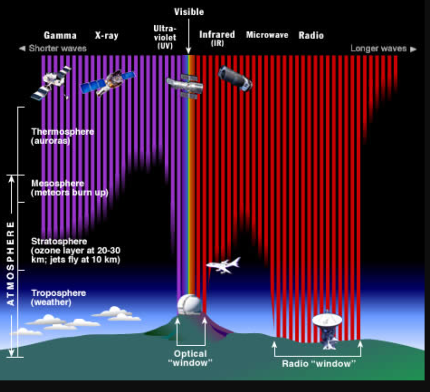
Various wavelengths of solar EM radiation penetrate Earth’s atmosphere to various depths. Fortunately for us, all of the high energy X-rays and most UV is filtered out long before it reaches the ground. Much of the infrared radiation is also absorbed by our atmosphere far above our heads. Most radio waves do make it to the ground, along with a narrow “window” of IR, UV, and visible light frequencies. Credit: Image courtesy STCI/JHU/NASA.

The co-author of the article was his boss at NASA Langley Research Center (Martin Mlynczak). Mlynczak put his name to the paper but did no work on it. He thought that it was an important paper, but only in a technical way.

When Miskolczi later informed the group at NASA there that he had more important results, they finally understood the whole story, and tried to withhold Miskolczi’s further material from publication. His boss for example, sat at Ferenc’s computer, logged in with Ferenc`s password, and canceled a recently submitted paper from a high-reputation journal as if Ferenc had withdrawn it himself. That was the reason that Ferenc finally resigned from his ($US 90,000 /year) job.

At the bottom of this post will be links to Miskolczi’s papers, including the latest one in 2014. Perhaps the most accessible introduction to his understanding comes from his interview with Kirk Myers published at Climate Truth.

Climate Truth: Has there been global warming?
Dr. Miskolczi: No one is denying that global warming has taken place, but it has nothing to do with the greenhouse effect or the burning of fossil fuels.

Climate Truth: According to the conventional anthropogenic global warming (AGW) theory, as human-induced CO2 emissions increase, more surface radiation is absorbed by the atmosphere, with part of it re-radiated to the earth’s surface, resulting in global warming. Is that an accurate description of the prevailing theory?
Dr. Miskolczi: Yes, this is the classic concept of the greenhouse effect.

ClimateTruth: Are man-made CO2 emissions the cause of global warming?
Dr. Miskolczi: Apparently not. According to my research, increases in CO2 levels have not increased the global-average absorbing power of the atmosphere.

ClimateTruth: Where does the traditional greenhouse theory make its fundamental mistake?
Dr. Miskolczi: The conventional greenhouse theory does not consider the newly discovered physical relationships involving infrared radiative fluxes. These relationships pose strong energetic constraints on an equilibrium system.

ClimateTruth: Why has this error escaped notice until now?
Dr. Miskolczi: Nobody thought that a 100-year-old theory could be wrong. The original greenhouse formula, developed by an astrophysicist, applies only to the stars, not to finite, semi-transparent planetary atmospheres. New equations had to be formulated.

ClimateTruth: According your theory, the greenhouse effect is self-regulating and stabilizes itself in response to rising CO2 levels. You identified (perhaps discovered) a “greenhouse constant” that keeps the greenhouse effect in equilibrium. Is that a fair assessment of your theory?
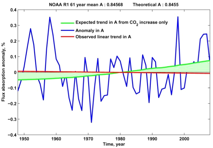
Dr. Miskolczi: Yes. Our atmosphere, with its infinite degree of freedom, is able to maintain its global average infrared absorption at an optimal level. In technical terms, this “greenhouse constant” is the total infrared optical thickness of the atmosphere, and its theoretical value is 1.87. Despite the 30 per cent increase of CO2 in the last 61 years, this value has not changed. The atmosphere is not increasing its absorption power as was predicted by the IPCC.

ClimateTruth: You used empirical data, rather than models, to arrive at your conclusion. How was that done?
Dr. Miskolczi: The computations are relatively simple. I collected a large number of radiosonde observations from around the globe and computed the global average infrared absorption. I performed these computations using observations from two large, publicly available datasets known as the TIGR2 and NOAA. The computations involved the processing of 300 radiosonde observations, using a state-of-the-art, line-by-line radiative transfer code. In both datasets, the global average infrared optical thickness turned out to be 1.87, agreeing with theoretical expectations.

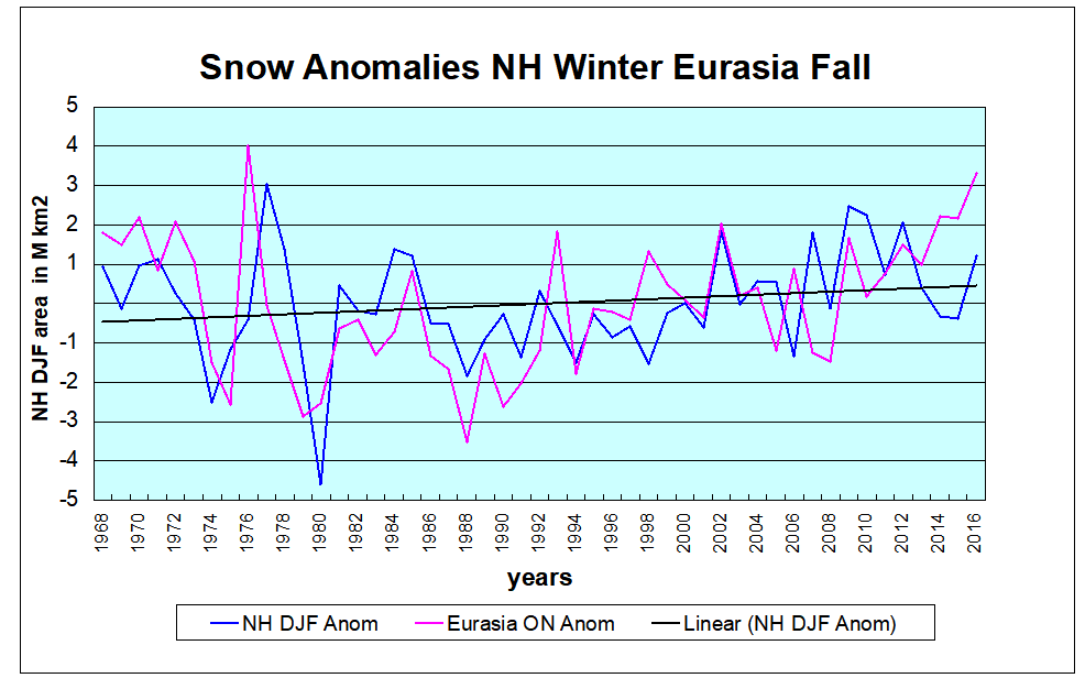
Fig. 15 the actual and expected atmospheric absorption trends are compared for the full time period. No change in the IR absorption is detected.

ClimateTruth: Have your mathematical equations been challenged or disproved?
Dr. Miskolczi: No.

ClimateTruth: If your theory stands up to scientific scrutiny, it would collapse the CO2 global warming doctrine and render meaningless its predictions of climate catastrophe. Given its significance, why has your theory been met with silence and, in some instances, dismissal and derision?
Dr. Miskolczi: I can only guess. First of all, nobody likes to admit mistakes. Second, somebody has to explain to the taxpayers why millions of dollars were spent on AGW research. Third, some people are making a lot of money from the carbon trade and energy taxes.

ClimateTruth: A huge industry has arisen out of the study and prevention of man-made global warming. Has the world been fooled?
Dr. Miskolczi: Thanks to censored science and the complicity of the mainstream media, yes, totally.
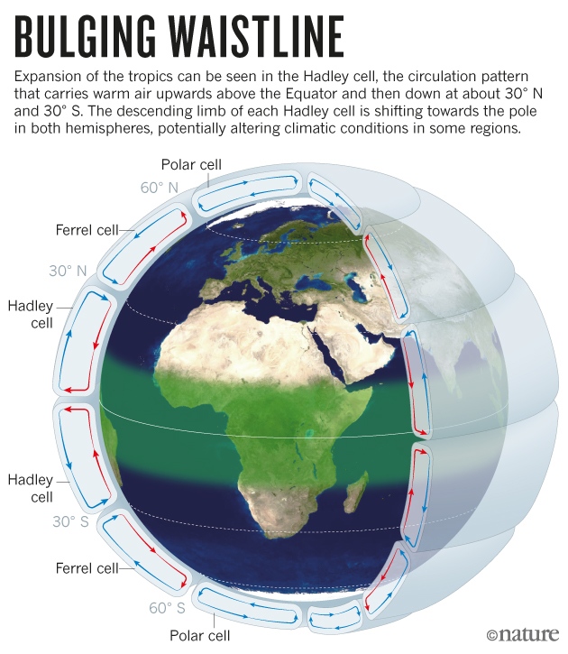
The Implications

Others have referred to Miskolczi’s work as finding a saturated greenhouse effect (not his terminology). Most people agree that gases have a logarithmic relation to IR absorption. Thus the effect of adding CO2, or H2O to the atmosphere has diminishing impact, like putting on another coat of paint.


Miskolczi’s analysis shows that at present CO2 concentrations, the radiative warming effect is saturated, because the atmospheric heat engine is always striving to maximize the dissipation of surface heat into space. In the present circumstance, any additional input of heat produces a reaction of additional evaporation or convection to restore the energy balance. Radiative equilibrium is not disturbed, as shown by the stability of the optical depth in the upper troposphere.

globalrelativehumidity300_700mb

This graph shows that the relative humidity has been dropping, especially at higher elevations allowing more heat to escape to space. The curve labelled 300 mb is at about 9 km altitude, which is in the middle of the predicted (but missing) tropical troposphere hot-spot. This is the critical elevation as this is where radiation can start to escape without being recaptured. The average annual relative humidity at this altitude has declined by 21.5% from 1948 to 2007.

If Miskolczi is right, then presently the land-sea surface heats the atmosphere only by evaporation, conduction, and subsequent convection, not by radiation. The layer of air in contact with the surface is in radiative equilibrium, so that warming and cooling of the surface is matched by the immediate air. The land-sea surface does not cool by radiation to the atmosphere, nor is it warmed by “back-radiation.”

Above the surface-air boundary, heat exchanges between layers of air do include radiative activity, and at the TOA it is all radiation into space. The climate system makes regulatory adjustment to compensate for changes in CO2 with changes in humidity and clouds, in order to most efficiently convert short wave incoming solar energy, into long wave outgoing energy. With warming and cooling periods, the proportions of H20 and CO2 at the TOA have fluctuated, but the combined optical depth has been stable over the last 60 years.

earth_energy_budget_ERBE
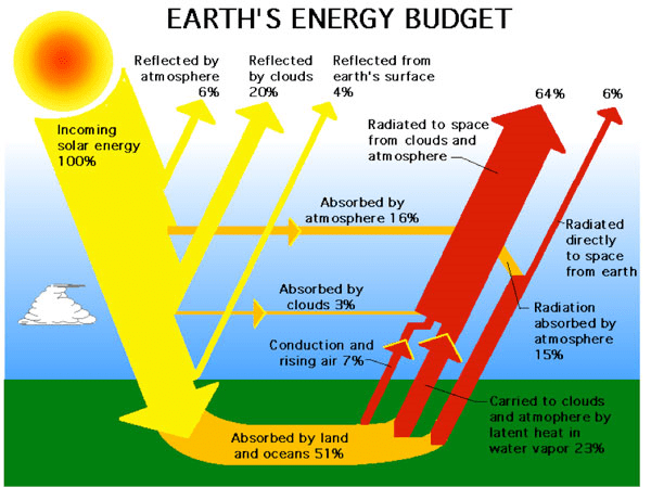
Credit: Image courtesy NASA’s ERBE (Earth Radiation Budget Experiment) program.

No wonder so much effort is going into a better understanding of cloud effects on climate.  Note in the above estimated energy budget diagram that convection and latent heat combined are twice the estimated surface radiation absorbed in the air.   Note also that the air absorbs more energy directly from the sun than it absorbs from the surface.

Bear in mind that water vapor does more than 90% of all IR activity by gases.  And note that clouds are composed of water droplets (liquid state), and IR activity by clouds (likely underestimated here) is on top of water’s thermal effect as a gas.

Summary: Dr. Ferenc Miskolczi’s  Strange Journey

Miskolczi’s story reads like a book. Looking at a series of differential equations for the greenhouse effect, he noticed the solution — originally done in 1922 by Arthur Milne, but still used by climate researchers today — ignored boundary conditions by assuming an “infinitely thick” atmosphere. Similar assumptions are common when solving differential equations; they simplify the calculations and often result in a result that still very closely matches reality. But not always.

So Miskolczi re-derived the solution, this time using the proper boundary conditions for an atmosphere that is not infinite. His result included a new term, which acts as a negative feedback to counter the positive forcing. At low levels, the new term means a small difference … but as greenhouse gases rise, the negative feedback predominates, forcing values back down.

NASA refused to release the results. Miskolczi believes their motivation is simple. “Money”, he tells DailyTech. Research that contradicts the view of an impending crisis jeopardizes funding, not only for his own atmosphere-monitoring project, but all climate-change research.

Miskolczi resigned in protest, stating in his October 28, 2005 resignation letter, “Unfortunately my working relationship with my NASA supervisors eroded to a level that I am not able to tolerate. My idea of the freedom of science cannot coexist with the recent NASA practice of handling new climate change related scientific results.”

“More than three years ago, I presented to NASA a new view of greenhouse theory and pointed out serious errors in the classical approach to assessing climate sensitivity to greenhouse gas perturbations. Since then my results were not released for publication. Since my new results have far reaching consequences in the general atmospheric radiative transfer, I wish to have no part in withholding the above scientific information from the wider community of scientists and policymakers.”
More at Cornwall Alliance Peer-Reviewed Research Suggests Very Little Warming from CO2

His theory was eventually published in a peer-reviewed scientific journal in his home country of Hungary.
The greenhouse effect and the spectral decomposition of the clear-sky terrestrial radiation

Miskolczi’s latest paper is The Greenhouse Effect and the Infrared Radiative Structure of the Earth’s Atmosphere 2014

Previously in 2010 he published in Energy & Environment The Stable Stationary Value of the Earth’s Global Average Atmospheric Planck-Weighted Greenhouse-Gas Optical Thickness

Dr. Ferenc Mark Miskolczi

Update May 18

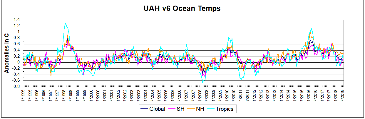
Robin Pittwood has done an analysis confirming that recent global warming has been matched by increasing outgoing longwave radiation, such that the equilibrium point has remained stable.  His money graph is this one:

This finding is consistent with Miskolczi’s finding that the atmospheric heat engine adjusts to changes so that energy balance is maintained.  There is more at KiwiThinker: An Empirical Look at Recent Trends in the Greenhouse Effect

CO2 ≠ Pollutant

My university degree is a Bachelors in Organic Chemistry from Stanford. For that and other reasons, it always annoyed me that some lawyers decided CO2 can be called a “pollutant”, all the while exhaling the toxic gas themselves.

This nonsense forms the root of all the ridiculous regulations that POTUS ordered reviewed and rescinded yesterday. Thus I agree completely with this Wall Street Journal article by Paul Tice Trump’s Next Step on Climate Change. Full text below.

Reconsider the EPA’s labeling of carbon dioxide as a pollutant, based on now-outdated science.

By PAUL H. TICE
March 28, 2017 6:41 p.m. ET

The executive orders on climate change President Trump signed this week represent a step in the right direction for U.S. energy policy and, importantly, deliver on Mr. Trump’s campaign promise to roll back burdensome regulations affecting American companies. But it will take more than the stroke of a pen to make lasting progress and reverse the momentum of the climate-change movement.

On Tuesday, in a series of orders, Mr. Trump instructed the Environmental Protection Agency to rework its Clean Power Plan, which would restrict carbon emissions from existing power plants, mainly coal-fired ones. Last year the U.S. Supreme Court stayed enforcement of the CPP pending judicial review.

Mr. Trump also directed the Interior Department to lift its current moratorium on federal coal leasing and loosen restrictions on oil and gas development (including methane flaring) on federal lands. And he instructed all government agencies to stop factoring climate change into the environmental-review process for federal projects. The federal government will recalculate the “social cost of carbon.”

These actions are a good start, but all they do is reverse many of the executive orders President Obama signed late in his second term. While easy to implement and theatrical to stage, such measures are largely superficial and may prove as temporary as the decrees they rescind.

Because they don’t attack the climate-change regulatory problem at its root, Mr. Trump’s orders will not provide enough clarity to U.S. energy companies—particularly electric utilities and coal-mining companies—for their long-term business forecasting or short-term capital investment and head-count planning.

To accomplish that, the Trump administration, led by EPA Administrator Scott Pruitt, needs to target the EPA’s 2009 “endangerment finding,” which labeled carbon dioxide as a pollutant. That foundational ruling provided the legal underpinnings for all of the EPA’s follow-on carbon regulations, including the CPP.

It also provided the rationale for the previous administration’s anti-fossil-fuel agenda and its various climate-change initiatives and programs, which spanned more than a dozen federal agencies and cost the American taxpayer roughly $20 billion to $25 billion a year during Mr. Obama’s presidency.

The endangerment finding was the product of a rush to judgment. Much of the scientific data upon which it was predicated—chiefly, the 2007 Fourth Assessment Report of the U.N.’s Intergovernmental Panel on Climate Change—was already dated by the time of its publication and arguably not properly peer-reviewed as federal law requires.

With the benefit of hindsight—including more than a decade of actual-versus-modeled data, plus the insights into the insular climate-science community gleaned from the University of East Anglia Climategate email disclosures—there would seem to be strong grounds now to reconsider the EPA’s 2009 decision and issue a new finding.

In 2013, the IPCC issued a more circumspect Fifth Assessment Report, which noted a hiatus in global warming since 1998 and a breakdown in correlation between the world’s average surface temperatures and atmospheric carbon dioxide levels, causing the U.N. body to revise down its 2007 projections for the rate of planetary warming over the first half of the 21st century.

Although this initially reported “pause” was subsequently eliminated through the downward manipulation of historical temperature data, this latest IPCC assessment calls into question both the predictive power and input data quality of most global climate models, and further highlights the scientific uncertainty surrounding the basic premise of anthropogenic climate change.

An updated EPA endangerment finding based on an objective review of the latest available scientific data is warranted, along with a more sober discussion of the threat posed by carbon dioxide and other greenhouse gases to the “public health and welfare of current and future generations,” in the words of the original endangerment finding.

As long as the 2009 finding remains on the books, it will provide legal ammunition for environmentalists, academics and state government officials seeking to sue the administration for any actions related to climate change, including this week’s executive orders.

Issuing a new endangerment finding would be a bold move requiring thorough work, but the Trump EPA would be well within its legal rights to undertake such an updated review process. In Massachusetts v. EPA (2007), the Supreme Court ruled that the Clean Air Act gives the EPA the authority, but not the obligation, to regulate carbon dioxide and other greenhouse gases. The EPA needs to “ground its reasons for action or inaction” with “reasoned judgment” and scientific analysis.

Addressing the 2009 endangerment finding head-on would show that Mr. Trump is serious about challenging climate-change orthodoxy. Thus far he has sent a mixed message, as demonstrated by this week’s ambivalence on CPP (reworking rather than repealing) and his administration’s silence on U.S. participation in the U.N.’s 2015 Paris Agreement.

Simply standing down on regulatory enforcement, cutting government funding for climate-change research and stopping data collection for the next four years will not suffice. Ignoring the EPA’s 2009 endangerment finding would mean that it is only a matter of time before another liberal-minded occupant of the White House reasserts this regulatory power, bringing the country and the domestic energy sector back where Mr. Obama left them.

Mr. Tice is an executive-in-residence at New York University’s Stern School of Business and a former Wall Street energy research analyst.