A comment by Dr. R.G. Brown of Duke University posted on June 11 at WUWT.
First about the way weather models work
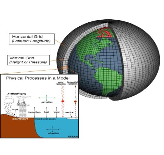
That is not quite what they do in GCMs. There are two reasons for this. One is that a global grid of 2 million temperatures sounds like a lot, but it’s not. Remember the atmosphere has depth, and they have to initialize at least to the top of the troposphere, and if they use 1 km thick cells there are 9 or 10 layers. Say 10. Then they have 500 million square kilometers of area to cover. Even if the grid itself has two million cells, that is still cells that contain 250 square km. This isn’t terrible — 16x16x1 km cells (20 million of them assuming they follow the usual practice of slabs 1 km thick) are small enough that they can actually resolve largish individual thunderstorms — but is still orders of magnitude larger than distinct weather features like individual clouds or smaller storms or tornadoes or land features (lakes, individual hills and mountains) that can affect the weather.
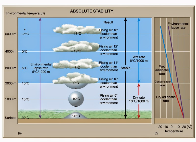
There is also substantial error in their initial conditions — as you say, they smooth temperatures sampled at a lot fewer than 2 million points to cover vast tracts of the grid where there simply are no thermometers, and even where they have surface thermometers they do not generally have soundings (temperature measurements from e.g. balloons that ride up the air column at a location) so they do not know the temperature in depth. The model initialization has to do things like take the surface temperature guess (from a smoothing model) and guess the temperature profile overhead using things like the adiabatic lapse rate, a comparative handful of soundings, knowledge of the cloudiness or whatever of the cell obtained from satellite or radar (where available) or just plain rules of thumb (all built into a model to initialize the model.
Then there is the ocean. Sea surface temperatures matter a great deal, but so do temperatures down to some depth (more for climate than for weather, but when large scale phenomena like hurricanes come along, the heat content of the ocean down to some depth very much plays a role in their development) so they have to model that, and the better models often contain at least one if not more layers down into the dynamic ocean. The Gulf Stream, for example, is a river in the Atlantic that transports heat and salinity and moves around 200 kilometers in a day on the surface, less at depth, which means that fluctuations in surface temperature, fed back or altered by precipitation or cloudiness or wind, move across many cells over the course of a day. (My Bold)
Even with all of the care I describe above and then some, weather models computed at close to the limits of our ability to compute (and get a decent answer faster than nature “computes” it by making it actually happen) track the weather accurately for a comparatively short time — days — before small variations between the heavily modeled, heavily under-sampled model initial conditions and the actual initial state of the weather plus errors in the computation due to many things — discrete arithmetic, the finite grid size, errors in the implementation of the climate dynamics at the grid resolution used (which have to be approximated in various ways to “mimic” the neglected internal smaller scaled dynamics that they cannot afford to compute) cause the models to systematically diverge from the actual weather.
If they run the model many times with small tweaks of the initial conditions, they have learned empirically that the distribution of final states they obtain can be reasonably compared to the climate for a few days more in an increasingly improbable way, until around a week or ten days out the variation is so great that they are just as well off predicting the weather by using the average weather for a date over the last 100 years and a bit of sense, just as is done in almanacs.
In other words, the models, no matter how many times they are run or how carefully they are initialized, produce results with no “lift” over ordinary statistics at around 10 days. (My bold)
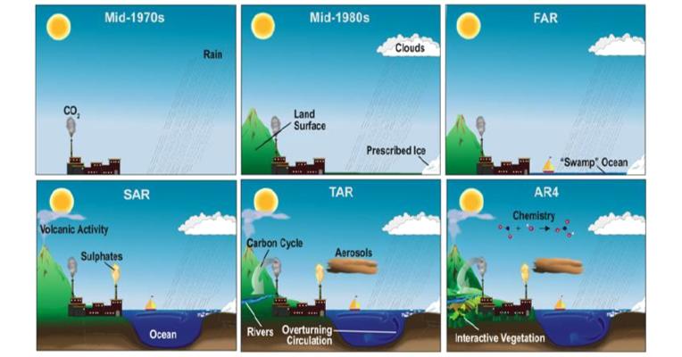
Evolution of state-of-the-art Climate Models from the mid 70s to the mid 00s. From IPCC (2007)
Now How Climate Models Work:
Then here is the interesting point. Climate models are just weather models run in exactly this way, with one exception. Since they know that the model will produce results indistinguishable from ordinary static statistics two weeks in, they don’t bother initializing them all that carefully. The idea is that no matter how then initialize them, after running them out to weeks or months the bundle of trajectories they produce from small perturbations will statistically “converge” at any given time to what is supposed to be the long time statistical average, which is what they are trying to predict.
This assumption is itself dubious, as neither the weather nor the climate is stationary and it is most definitely non-Markovian so that the neglected details in the initial state do matter in the evolution of both, and there is also no theorem of which I am aware that states that the average or statistical distribution of a bundle of trajectories generated from a nonlinear chaotic model of this sort will in even the medium run be an accurate representation of the nonstationary statistical distribution of possible future climates. But it’s the only game in town, so they give it a try.
They then run this re-purposed, badly initialized weather model out until they think it has had time to become a “sample” for the weather for some stationary initial condition (fixed date, sunlight, atmosphere, etc) and then they vary things like CO_2 systematically over time while integrating and see how the run evolves over future decades. The bundle of future climate trajectories thus generated from many tweaks of initial conditions and sometimes the physical parameters as well is then statistically analyzed, and its mean becomes the central prediction of the model and the variance or envelope of all of the trajectories become confidence intervals of its predictions.
The problem is that they aren’t really confidence intervals because we don’t really have any good reason to think that the integration of the weather ten years into the future at an inadequate grid size, with all of the accumulation of error along the way, is actually a sample from the same statistical distribution that the real weather is being drawn from subject to tiny perturbations in its initial state. The climate integrates itself down to the molecular level, not on a 16×16 km grid, and climate models can’t use that small a grid size and run in less than infinite time, so the highest resolution I’ve heard of is 100×100 km^2 cells (10^4 square km, which is around 50,000 cells, not two million).
At this grid size they cannot see individual thunderstorms at all. Indeed, many extremely dynamic features of heat transport in weather have to be modeled by some sort of empirical “mean field” approximation of the internal cell dynamics — “average thunderstormicity” or the like as thunderstorms in particular cause rapid vertical transport of a lot of heat up from the surface and rapid transport of chilled/chilling water down to the surface, among other things. The same is true of snowpack — even small errors in average snowpack coverage make big differences in total heat received in any given winter and this can feed back to kick a model well off of the real climate in a matter of years.
So far, it looks like (not unlike the circumstance with weather) climate models can sometimes track the climate for a decade or so before they diverge from it. (My Bold)
They suffer from many other ailments as well — if one examines the actual month to month or year to year variance of the “weather” they predict, it has the wrong amplitude and decay times compared to the actual climate, which is basically saying (via the fluctuation-dissipation theorem) that they have the physics of the open system wrong. The models heavily exaggerate the effect of aerosols and tend to overreact to things like volcanic eruptions that dump aerosols into the atmosphere.
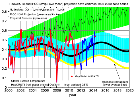
The models are tuned to cancel the exaggerated effect of aerosols with an exaggerated feedback on top of CO_2 driven warming to make them “work” to track the climate over a 20 year reference period. Sadly, this 20 year reference period was chosen to be the single strongest warming stretch of the 20th century, ignoring cooling periods and warming periods that preceded it and (probably as a consequence) diverging from the flat-to-slightly cooling period we’ve been in for the last 16 or so years (or more, or less, depending on who you are talking to, but even the IPCC formally recognizes “the pause, the hiatus”, the lack of warming for this interval, in AR5. It is a serious problem for the models and everybody knows it.
The IPCC then takes the results of many GCMs and compounds all errors by super-averaging their results (which has the effect of hiding the fluctuation problem from inquiring eyes), ignoring the fact that some models in particular truly suck in all respects at predicting the climate and that others do much better, because the ones that do better predict less long run warming and that isn’t the message they want to convey to policy makers, and transform its envelope into a completely unjustifiable assertion of “statistical confidence”.
This is a simple lie. Each model one at a time can have the confidence interval produced by the spread in long-run trajectories produced by the perturbation of its initial conditions compared to the actual trajectory of the climate and turned into a p-value. The p-value is a measure of the probability of the truth of the null hypothesis — “This climate model is a perfect model in that its bundle of trajectories is a representation of the actual distribution of future climates”. This permits the estimation of the probability of getting our particular real climate given this distribution, and if the probability is low, especially if it is very low, we under ordinary circumstances would reject the huge bundle of assumptions tied up in as “the hypothesis” represented by the model itself and call the model “failed”, back to the drawing board.
One cannot do anything with the super-average of 36 odd non-independent grand average per-model results. To even try to apply statistics to this shotgun blast of assumptions one has to use something called the Bonferroni correction, which basically makes the p-value for failure of individual models in the shotgun blast much, much larger (because they have 36 chances to get it right, which means that even if all 36 are wrong pure chance can — no, probably will — make a bad model come out within a p = 0.05 cutoff as long as the models aren’t too wrong yet.
By this standard, “the set of models in CMIP5″ has long since failed. There isn’t the slightest doubt that their collective prediction is statistical nonsense. It remains to be seen if individual models in the collection deserve to be kept in the running as not failed yet, because even applying the Bonferroni correction to the “ensemble” of CMIP5 is not good statistical practice. Each model should really be evaluated on its own merits as one doesn’t expect the “mean” or “distribution” of individual model results to have any meaning in statistics (note that this is NOT like perturbing the initial conditions of ONE model, which is a form of Monte Carlo statistical sampling and is something that has some actual meaning).
Hope this helps.
rgb
http://wattsupwiththat.com/2015/06/09/huge-divergence-between-latest-uah-and-hadcrut4-revisions-now-includes-april-data/#comment-1960561
In the conclusion of a recent paper, Valerio Lucarini adds:
We have briefly recapitulated some of the scientific challenges and epistemological issues related to climate science. We have discussed the formulation and testing of theories and numerical models, which, given the presence of unavoidable uncertainties in observational data, the nonrepeatability of world-experiments, and the fact that relevant processes occur in a large variety of spatial and temporal scales, require a rather different approach than in other scientific contexts.
In particular, we have clarified the presence of two different levels of unavoidable uncertainties when dealing with climate models, related to the complexity and chaoticity of the system under investigation. The first is related to the imperfect knowledge of the initial conditions, the second is related to the imperfect representation of the processes of the system, which can be referred to as structural uncertainties of the model. We have discussed how Monte Carlo methods provide partial but very popular solutions to these problems. A third level of uncertainty is related to the need for a, definitely non-trivial, definition of the appropriate metrics in the process of validation of the climate models. We have highlighted the difference between metrics aimed at providing information of great relevance for the end-user from those more focused on the audit of the most important physical processes of the climate system.
It is becoming clearer and clearer that the current strategy of incremental improvements of climate models is failing to produce a qualitative change in our ability to describe the climate system, also because the gap between the simulation and the understanding of the climate system is widening (Held 2005, Lucarini 2008a). Therefore, the pursuit of a “quantum leap” in climate modeling – which definitely requires new scientific ideas rather than just faster supercomputers – is becoming more and more of a key issue in the climate community (Shukla et al. 2009).
Lucarini goes further: Our proposal: a Thermodynamic perspective
While acknowledging the scientific achievements obtained along the above mentioned line, we propose a different approach for addressing the big picture of a complex system like climate is. An alternative way for providing a new, satisfactory theory of climate dynamics able to tackle simultaneously balances of physical quantities and dynamical instabilities is to adopt a thermodynamic perspective, along the lines proposed by Lorenz (1967). We consider simultaneously two closely related approaches, a phenomenological outlook based on the macroscopic theory of non-equilibrium thermodynamics (see e.g., de Groot and Mazur 1962), and, a more fundamental outlook, based on the paradigm of ergodic theory (Eckmann and Ruelle 1985) and more recent developments of the non-equilibrium statistical mechanics (Ruelle 1998, 2009).
The concept of the energy cycle of the atmosphere introduced by Lorenz (1967) allowed for defining an effective climate machine such that the atmospheric and oceanic motions simultaneously result from the mechanical work (then dissipated in a turbulent cascade) produced by the engine, and re-equilibrate the energy balance of the climate system. One of the fundamental reasons why a comprehensive understanding of climate dynamics is hard to achieve lies on the presence of such a nonlinear closure. Recently, Johnson (2000) introduced a Carnot engine–equivalent picture of the climate system by defining effective warm and the cold reservoirs and their temperatures.

From Modelling Complexity: the case of Climate Science, V. Lucarini
Click to access 1106.1265.pdf
For more on Climate models see:
https://rclutz.wordpress.com/2015/03/24/temperatures-according-to-climate-models/
https://rclutz.wordpress.com/2015/03/25/climate-thinking-out-of-the-box/


 hat tip to Homer Simpson

