Wyoming: Make Carbon Dioxide Great Again–No Net Zero

A bill is progressing through the Wyoming State Legislature, as described by the author in her op-ed Rethinking Carbon Dioxide – Wyoming’s Bold Move.  Excerpts in italics with my bolds and added images.

Torrington, WY (State Senator Cheri Steinmetz) January 7th, 2025 — The people of Wyoming have always believed in the value of questioning conventional wisdom, looking at the bigger picture and finding solutions that are possible and actually work. That’s the purpose of the bill titled “Make Carbon Dioxide Great Again”. This legislation is not about denying science, it is about applying science, thoroughly reevaluating the ‘climate change’ scientific assumptions and advocating for policies grounded in practicality, reality, and achievability – common sense.

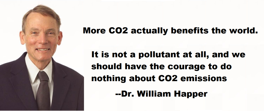
Carbon dioxide (CO2) is vital to life on Earth.

Without it, plants could not grow, and without plants, no life would survive. Scientists and farmers alike recognize that higher CO2 levels improve agricultural productivity. Plants thrive with more CO2 – they grow faster, use water more efficiently, and are more resilient to drought. NASA’s own research shows that rising CO2 has contributed to a global “greening” effect, expanding vegetation and helping ecosystems flourish. CO2 is plant food!

Yet, despite its essential role in sustaining life,
CO2 has been demonized as a pollutant.

But what impact are human driven CO2 emissions actually capable of? We are contributing a very small part of the natural carbon cycle. Current CO2 levels are among the lowest Earth has seen over its long history. There were times in the past when ecosystems flourished under much higher CO2 concentrations. Instead of vilifying this essential gas, we should be acknowledging its role in our ecosystems and industries and protect the benefits it has in our lives.

Wyoming is uniquely positioned to lead this conversation.

Our state is vital to energy production, agriculture and food industries, transportation and energy reliability and stability. We understand the real-world importance of CO2. And we understand the benefits of CO2 used directly. Our industries already use it to enhance oil recovery, making energy production more efficient. This technology exemplifies what we are capable of when we treat CO2 as a resource rather than a liability.

The bill Make Carbon Dioxide Great Again shifts how we think about CO2.

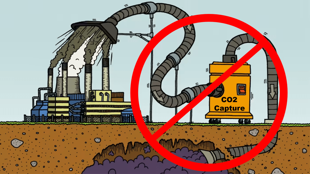
It proposes that we stop treating the essential gas as a pollutant or contaminant. It requires a clear-eyed look at how policies aimed at eliminating CO2 emissions, such as decarbonizing the West, making Wyoming carbon negative or popular “net-zero” mandates. They may sound good on paper but often come with high economic costs and questionable environmental benefits, and clearly negative effects on our people and our industries.

Wyoming must refuse to jeopardize our economy and energy security
for initiatives that will yield – at best – questionable results.

Critics of “net-zero” strategies have highlighted the risks of pursuing policy goals without fully considering their consequences. These frequently require massive investments, disruption of reliable energy systems, and the forced undue burdens on families and businesses. Instead, Wyoming advocates for a balanced approach – one that evaluates the risks and possible rewards of any CO2 management plans that will safeguard our economic stability and way of life.

This approach challenges the status quo, and that is precisely the point. Now is the time to rethink how we talk about CO2 and climate change. This bill is not about ignoring environmental concerns; it is about addressing them with clear-eyed pragmatism and truth.

Wyoming is taking a bold step forward to lead a balanced, science-based dialogue. We all stand to benefit from this. Our energy sector, agriculture, transportation and all other industries, and even the broader environment, will gain when we use CO2 wisely.

This conversation is just beginning and must spark
a national debate about the fundamental role of CO2.

It is a debate we need to have – not just in Wyoming, with our own Governor and citizens – but across the nation and with all the organizations leading the charge to “net zero.” Let us challenge the assumptions, ask the hard questions, and make sure our policies truly serve the people, industry and the environment. After all, that is the Wyoming way.

Text of Wyoming Bill     SF0092  Make carbon dioxide great again-no net zero.

AN   ACT   relating to   environmental quality;   providing legislative findings;
specifying that carbon dioxide is not a pollutant and is a beneficial substance;
providing policy statements of the state associated with carbon dioxide;
repealing low-carbon energy standard requirements; repealing conflicting provisions;
making conforming amendments;  specifying applicability;
requiring reimbursement to utility customers as specified;
requiring rulemaking; and providing for an effective date.

Be It Enacted by the Legislature of the State of Wyoming:

Section 1.    W.S. 35-11-215 is created to read:

1             SF0092

35-11-215.     Carbon dioxide;   beneficial treatment; state policy.

(a)   The legislature finds that:

  (i)    Carbon dioxide is  a foundational nutrient necessary for all life on earth. Plants need carbon dioxide along with sunlight, water and nutrients to prosper. The more carbon dioxide available for this, the better life can  flourish;

  (ii)    The carbon cycle, where carbon dioxide is reused and transferred between the atmosphere and organisms on earth, is a biological necessity for life on earth;

  (iii)    Agricultural production worldwide is outpacing population growth and breaking production records primarily due to increasing atmospheric carbon dioxide;

  (iv)    More carbon dioxide allows plants to better resist drought by using water more efficiently;

  (v)     The national aeronautics and space administration has confirmed that global vegetation is increasing from the near-polar regions to the equator. The largest contributor to this greening of  the earth is increasing carbon dioxide;

  (vi)     Carbon dioxide levels are currently at approximately four hundred twenty (420) parts per million, which is  at near-historically low concentrations.   The current carbon dioxide levels are one-sixth (1/6) of the average of  two thousand six hundred  (2,600)  parts per million over geologic time;

  (vii)     It is estimated that carbon dioxide levels  need to exceed one hundred fifty (150) parts per million to ensure the survival of plant life on earth;

  (viii)     The earth needs carbon dioxide to support  life and to  increase plant yields,  both of     which will contribute to  the health and prosperity of  all Wyoming citizens.

   (b)     It is the policy of the state of Wyoming that:

(i)       Carbon dioxide is a foundational nutrient necessary for life on earth;

(ii)       Carbon dioxide shall not be designated or treated as a pollutant or contaminant;

(iii)       The state of Wyoming shall not pursue any targets or measures that support the reduction or elimination of  carbon dioxide,  including any  “net-zero”  targets.

          Section 2.        W.S. 37-1-101(a)(intro) and 37-2-134(a)(i)  and (iv) are amended to read:

37-1-101.       Definitions.

(a)   As used in chapters 1, 2, 3, 12, and 17 and 18 of  this title:

37-2-134.       Electric generation facility closures; presumption; commission review

(a)    As used in this section:

(i)     “Dispatchable” means as defined in W.S. 37-18-101(a)(ii) a source of electricity that is available for use on demand and that can be dispatched upon request of a power grid operator or that can have its power output adjusted, according to  market needs and includes dispatchability;

(iv)    “Reliable” means as  defined in W.S. 37-18-101(a)(iv) generated electricity that is not subject to intermittent availability.

        Section    3.    W.S.    37-1-101(a)(vi)(N), 37-18-101 and  37-18-102 are repealed.

Section    4.   Not later than sixty (60) days after the effective date of this act each public utility that recovered rates from customers under W.S. 37-18-102(c)(i) or (iii),  as repealed by section 3 of this act, shall refund those rates to customers who paid them, provided that the utility shall not be  required to refund rates recovered under W.S. 37-18-102(c)(i) and (iii) that the utility had expended for carbon capture, utilization and storage technology before the effective date of this act. Refunds required under this section shall be in a form and manner specified by the public service commission

Section    5.  The public service commission shall promulgate all rules necessary to implement this act.

Section    6.  This act is effective immediately upon completion of all acts necessary for a bill to become law as provided by Article 4, Section 8 of the Wyoming Constitution.

 (END)

Ocean Even Cooler December 2024

The best context for understanding decadal temperature changes comes from the world’s sea surface temperatures (SST), for several reasons:

  • The ocean covers 71% of the globe and drives average temperatures;
  • SSTs have a constant water content, (unlike air temperatures), so give a better reading of heat content variations;
  • Major El Ninos have been the dominant climate feature in recent years.

HadSST is generally regarded as the best of the global SST data sets, and so the temperature story here comes from that source. Previously I used HadSST3 for these reports, but Hadley Centre has made HadSST4 the priority, and v.3 will no longer be updated.  HadSST4 is the same as v.3, except that the older data from ship water intake was re-estimated to be generally lower temperatures than shown in v.3.  The effect is that v.4 has lower average anomalies for the baseline period 1961-1990, thereby showing higher current anomalies than v.3. This analysis concerns more recent time periods and depends on very similar differentials as those from v.3 despite higher absolute anomaly values in v.4.  More on what distinguishes HadSST3 and 4 from other SST products at the end. The user guide for HadSST4 is here.

The Current Context

The chart below shows SST monthly anomalies as reported in HadSST4 starting in 2015 through December 2024.  A global cooling pattern is seen clearly in the Tropics since its peak in 2016, joined by NH and SH cycling downward since 2016, followed by rising temperatures in 2023 and 2024.

Note that in 2015-2016 the Tropics and SH peaked in between two summer NH spikes.  That pattern repeated in 2019-2020 with a lesser Tropics peak and SH bump, but with higher NH spikes. By end of 2020, cooler SSTs in all regions took the Global anomaly well below the mean for this period.  A small warming was driven by NH summer peaks in 2021-22, but offset by cooling in SH and the tropics, By January 2023 the global anomaly was again below the mean.

Now in 2023-24 came an event resembling 2015-16 with a Tropical spike and two NH spikes alongside, all higher than 2015-16. There was also a coinciding rise in SH, and the Global anomaly was pulled up to 1.1°C last year, ~0.3° higher than the 2015 peak.  Then NH started down autumn 2023, followed by Tropics and SH descending 2024 to the present. After 10 months of cooling in SH and the Tropics, the Global anomaly came back down, led by NH cooling the last 4 months from its peak in August. It’s now about 0.1C higher than the average for this period. Note that the Tropical anomaly has cooled from 1.29C in 2024/01 to 0.66C as of 2024/12.

Comment:

The climatists have seized on this unusual warming as proof their Zero Carbon agenda is needed, without addressing how impossible it would be for CO2 warming the air to raise ocean temperatures.  It is the ocean that warms the air, not the other way around.  Recently Steven Koonin had this to say about the phonomenon confirmed in the graph above:

El Nino is a phenomenon in the climate system that happens once every four or five years.  Heat builds up in the equatorial Pacific to the west of Indonesia and so on.  Then when enough of it builds up it surges across the Pacific and changes the currents and the winds.  As it surges toward South America it was discovered and named in the 19th century  It iswell understood at this point that the phenomenon has nothing to do with CO2.

Now people talk about changes in that phenomena as a result of CO2 but it’s there in the climate system already and when it happens it influences weather all over the world.   We feel it when it gets rainier in Southern California for example.  So for the last 3 years we have been in the opposite of an El Nino, a La Nina, part of the reason people think the West Coast has been in drought.

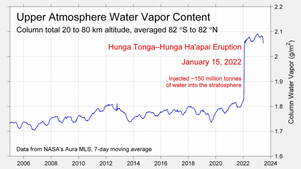
It has now shifted in the last months to an El Nino condition that warms the globe and is thought to contribute to this Spike we have seen. But there are other contributions as well.  One of the most surprising ones is that back in January of 2022 an enormous underwater volcano went off in Tonga and it put up a lot of water vapor into the upper atmosphere. It increased the upper atmosphere of water vapor by about 10 percent, and that’s a warming effect, and it may be that is contributing to why the spike is so high.

A longer view of SSTs

Open image in new tab to enlarge.

The graph above is noisy, but the density is needed to see the seasonal patterns in the oceanic fluctuations.  Previous posts focused on the rise and fall of the last El Nino starting in 2015.  This post adds a longer view, encompassing the significant 1998 El Nino and since.  The color schemes are retained for Global, Tropics, NH and SH anomalies.  Despite the longer time frame, I have kept the monthly data (rather than yearly averages) because of interesting shifts between January and July. 1995 is a reasonable (ENSO neutral) starting point prior to the first El Nino. 

The sharp Tropical rise peaking in 1998 is dominant in the record, starting Jan. ’97 to pull up SSTs uniformly before returning to the same level Jan. ’99. There were strong cool periods before and after the 1998 El Nino event. Then SSTs in all regions returned to the mean in 2001-2. 

SSTS fluctuate around the mean until 2007, when another, smaller ENSO event occurs. There is cooling 2007-8,  a lower peak warming in 2009-10, following by cooling in 2011-12.  Again SSTs are average 2013-14.

Now a different pattern appears.  The Tropics cooled sharply to Jan 11, then rise steadily for 4 years to Jan 15, at which point the most recent major El Nino takes off.  But this time in contrast to ’97-’99, the Northern Hemisphere produces peaks every summer pulling up the Global average.  In fact, these NH peaks appear every July starting in 2003, growing stronger to produce 3 massive highs in 2014, 15 and 16.  NH July 2017 was only slightly lower, and a fifth NH peak still lower in Sept. 2018.

The highest summer NH peaks came in 2019 and 2020, only this time the Tropics and SH were offsetting rather adding to the warming. (Note: these are high anomalies on top of the highest absolute temps in the NH.)  Since 2014 SH has played a moderating role, offsetting the NH warming pulses. After September 2020 temps dropped off down until February 2021.  In 2021-22 there were again summer NH spikes, but in 2022 moderated first by cooling Tropics and SH SSTs, then in October to January 2023 by deeper cooling in NH and Tropics.  

Then in 2023 the Tropics flipped from below to well above average, while NH produced a summer peak extending into September higher than any previous year.  Despite El Nino driving the Tropics January 2024 anomaly higher than 1998 and 2016 peaks, following months cooled in all regions, and the Tropics continued cooling in April, May and June along with SH dropping.  After July and August NH warming again pulled the global anomaly higher, September and October resumed cooling in all regions.

What to make of all this? The patterns suggest that in addition to El Ninos in the Pacific driving the Tropic SSTs, something else is going on in the NH.  The obvious culprit is the North Atlantic, since I have seen this sort of pulsing before.  After reading some papers by David Dilley, I confirmed his observation of Atlantic pulses into the Arctic every 8 to 10 years.

Contemporary AMO Observations

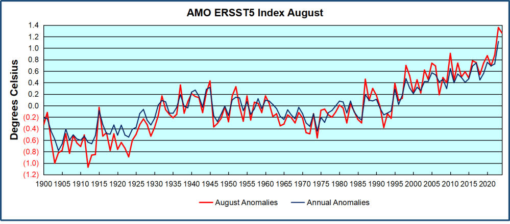
Through January 2023 I depended on the Kaplan AMO Index (not smoothed, not detrended) for N. Atlantic observations. But it is no longer being updated, and NOAA says they don’t know its future.  So I find that ERSSTv5 AMO dataset has current data.  It differs from Kaplan, which reported average absolute temps measured in N. Atlantic.  “ERSST5 AMO  follows Trenberth and Shea (2006) proposal to use the NA region EQ-60°N, 0°-80°W and subtract the global rise of SST 60°S-60°N to obtain a measure of the internal variability, arguing that the effect of external forcing on the North Atlantic should be similar to the effect on the other oceans.”  So the values represent sst anomaly differences between the N. Atlantic and the Global ocean.

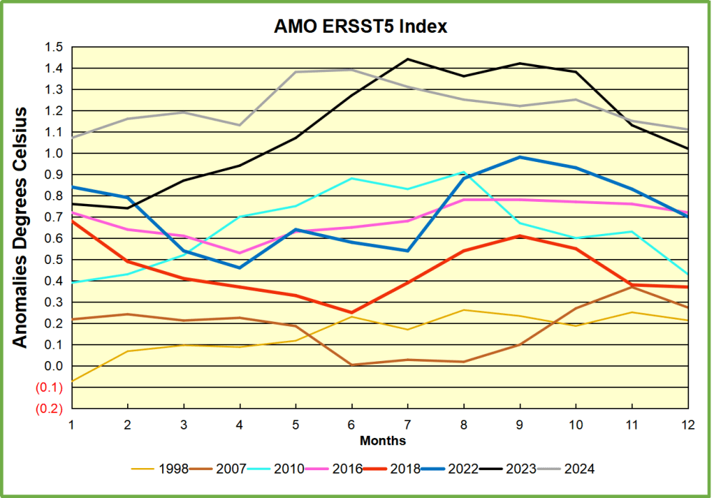
The chart above confirms what Kaplan also showed.  As August is the hottest month for the N. Atlantic, its variability, high and low, drives the annual results for this basin.  Note also the peaks in 2010, lows after 2014, and a rise in 2021. Then in 2023 the peak was holding at 1.4C before declining.  An annual chart below is informative:

Note the difference between blue/green years, beige/brown, and purple/red years.  2010, 2021, 2022 all peaked strongly in August or September.  1998 and 2007 were mildly warm.  2016 and 2018 were matching or cooler than the global average.  2023 started out slightly warm, then rose steadily to an  extraordinary peak in July.  August to October were only slightly lower, but by December cooled by ~0.4C.

Then in 2024 the AMO anomaly started higher than any previous year, then leveled off for two months declining slightly into April.  Remarkably, May showed an upward leap putting this on a higher track than 2023, and rising slightly higher in June.  In July, August and September 2024 the anomaly declined, and despite a small rise in October, is now lower than the peak reached in 2023.

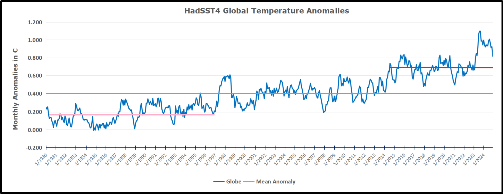
The pattern suggests the ocean may be demonstrating a stairstep pattern like that we have also seen in HadCRUT4. 

The purple line is the average anomaly 1980-1996 inclusive, value 0.18.  The orange line the average 1980-2024, value 0.39, also for the period 1997-2012. The red line is 2013-2024, value 0.67. As noted above, these rising stages are driven by the combined warming in the Tropics and NH, including both Pacific and Atlantic basins.

See Also:

2024 El Nino Collapsing

Curiosity:  Solar Coincidence?

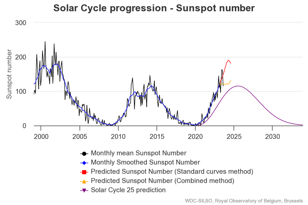
The news about our current solar cycle 25 is that the solar activity is hitting peak numbers now and higher  than expected 1-2 years in the future.  As livescience put it:  Solar maximum could hit us harder and sooner than we thought. How dangerous will the sun’s chaotic peak be?  Some charts from spaceweatherlive look familar to these sea surface temperature charts.

Summary

The oceans are driving the warming this century.  SSTs took a step up with the 1998 El Nino and have stayed there with help from the North Atlantic, and more recently the Pacific northern “Blob.”  The ocean surfaces are releasing a lot of energy, warming the air, but eventually will have a cooling effect.  The decline after 1937 was rapid by comparison, so one wonders: How long can the oceans keep this up? And is the sun adding forcing to this process?

Space weather impacts the ionosphere in this animation. Credits: NASA/GSFC/CIL/Krystofer Kim

Footnote: Why Rely on HadSST4

HadSST is distinguished from other SST products because HadCRU (Hadley Climatic Research Unit) does not engage in SST interpolation, i.e. infilling estimated anomalies into grid cells lacking sufficient sampling in a given month. From reading the documentation and from queries to Met Office, this is their procedure.

HadSST4 imports data from gridcells containing ocean, excluding land cells. From past records, they have calculated daily and monthly average readings for each grid cell for the period 1961 to 1990. Those temperatures form the baseline from which anomalies are calculated.

In a given month, each gridcell with sufficient sampling is averaged for the month and then the baseline value for that cell and that month is subtracted, resulting in the monthly anomaly for that cell. All cells with monthly anomalies are averaged to produce global, hemispheric and tropical anomalies for the month, based on the cells in those locations. For example, Tropics averages include ocean grid cells lying between latitudes 20N and 20S.

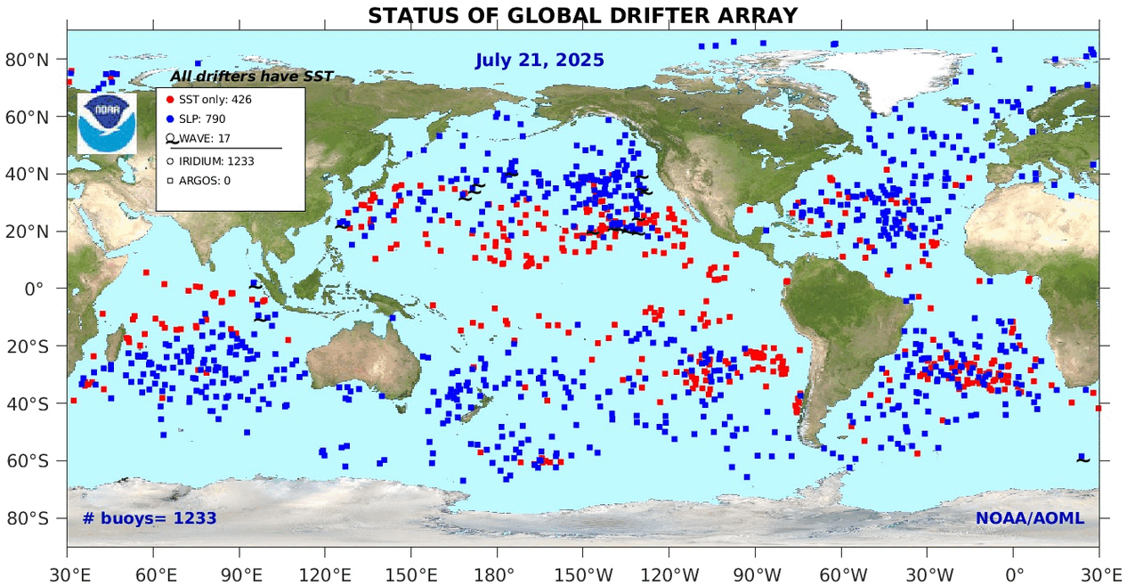
Gridcells lacking sufficient sampling that month are left out of the averaging, and the uncertainty from such missing data is estimated. IMO that is more reasonable than inventing data to infill. And it seems that the Global Drifter Array displayed in the top image is providing more uniform coverage of the oceans than in the past.

uss-pearl-harbor-deploys-global-drifter-buoys-in-pacific-ocean

USS Pearl Harbor deploys Global Drifter Buoys in Pacific Ocean


12/2024 Update–As Temperature Changes, CO2 Follows

Previously I have demonstrated that changes in atmospheric CO2 levels follow changes in Global Mean Temperatures (GMT) as shown by satellite measurements from University of Alabama at Huntsville (UAH). That background post is reprinted later below.

My curiosity was piqued by the remarkable GMT spike starting in January 2023 and rising to a peak in April 2024, and then declining afterward.  I also became aware that UAH has recalibrated their dataset due to a satellite drift that can no longer be corrected. The values since 2020 have shifted slightly in version 6.1, as shown in my recent report  Ocean Leads Cooling UAH December 2024.

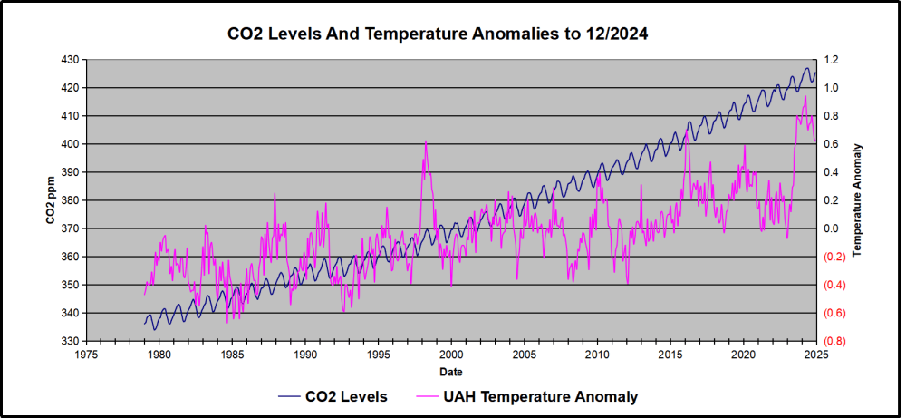
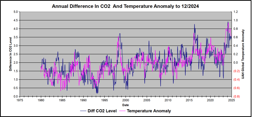
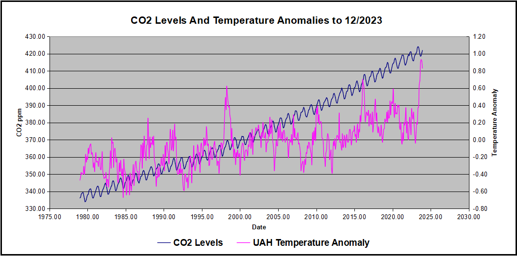
In this post, I test the premise that temperature changes are predictive of changes in atmospheric CO2 concentrations.  The chart above shows the two monthly datasets: CO2 levels in blue reported at Mauna Loa, and Global temperature anomalies in purple reported by UAHv6.1, both through December 2024. Would such a sharp increase in temperature be reflected in rising CO2 levels, according to the successful mathematical forecasting model? Would CO2 levels decline as temperatures dropped following the peak?

The answer is yes: that temperature spike resulted
in a corresponding CO2 spike as expected.
And lower CO2 levels followed the temperature decline.

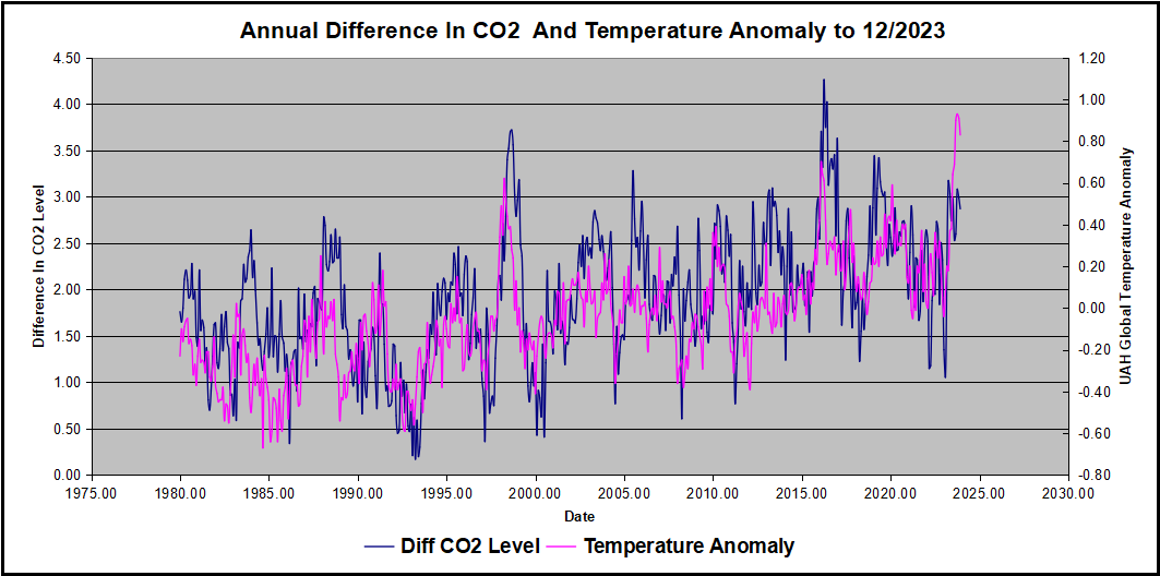
Above are UAH temperature anomalies compared to CO2 monthly changes year over year.

Changes in monthly CO2 synchronize with temperature fluctuations, which for UAH are anomalies now referenced to the 1991-2020 period. CO2 differentials are calculated for the present month by subtracting the value for the same month in the previous year (for example December 2024 minus December 2023).  Temp anomalies are calculated by comparing the present month with the baseline month. Note the recent CO2 upward spike and drop following the temperature spike and drop.

The final proof that CO2 follows temperature due to stimulation of natural CO2 reservoirs is demonstrated by the ability to calculate CO2 levels since 1979 with a simple mathematical formula:

For each subsequent year, the CO2 level for each month was generated

CO2  this month this year = a + b × Temp this month this year  + CO2 this month last year

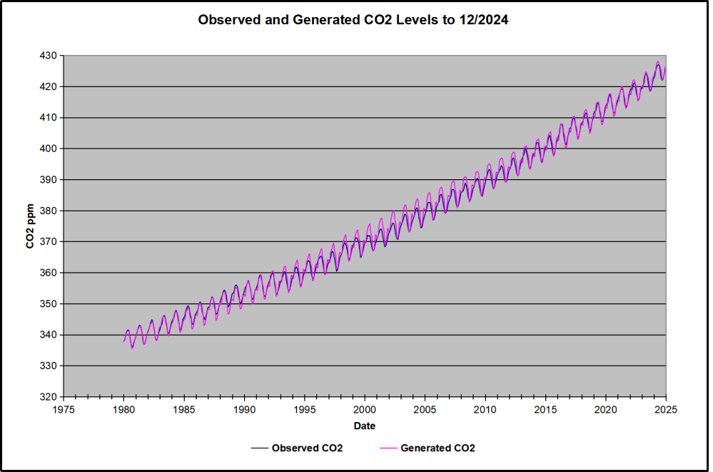
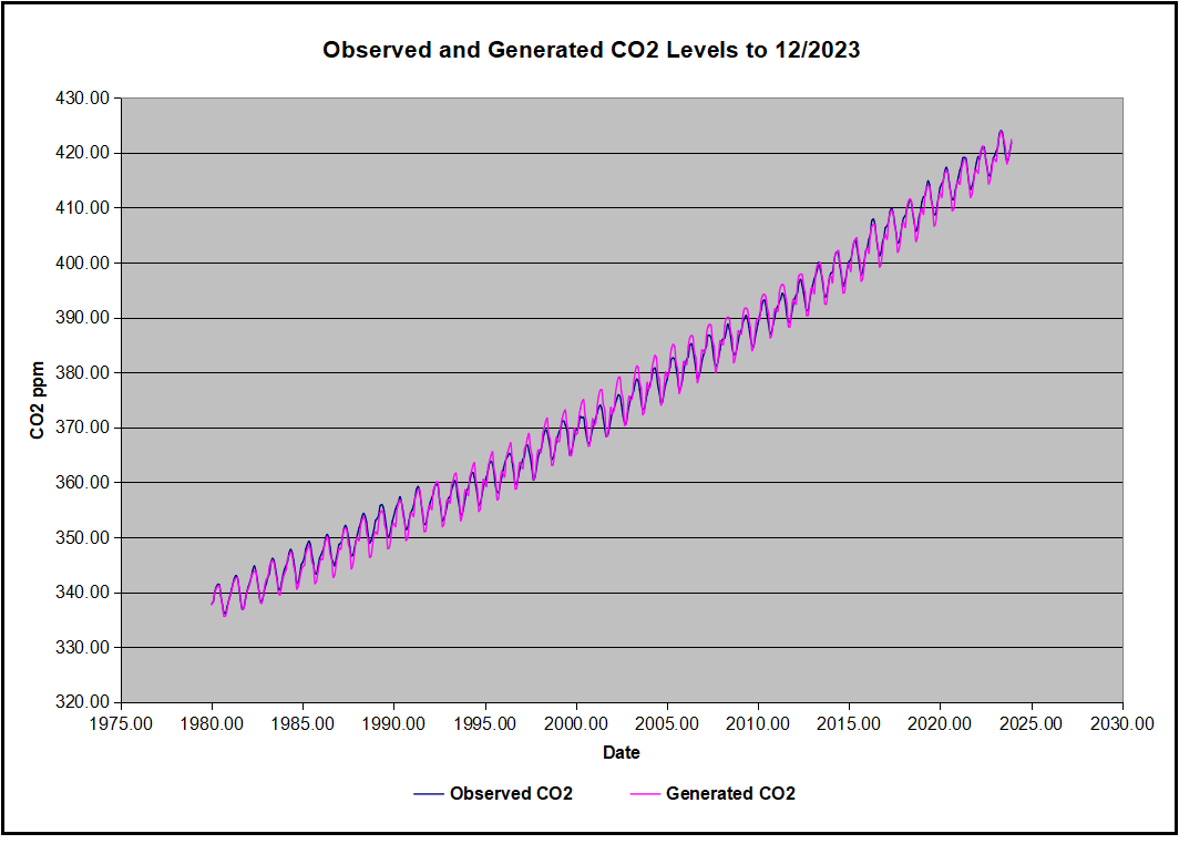
The values for a and b are constants applied to all monthly temps, and are chosen to scale the forecasted CO2 level for comparison with the observed value. Here is the result of those calculations.

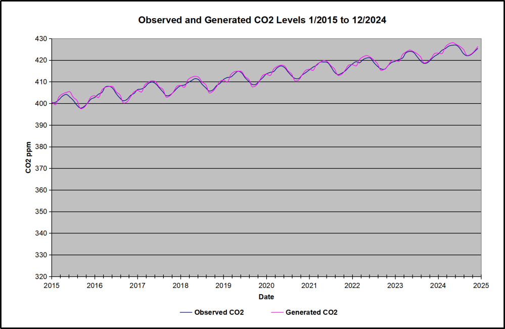
In the chart calculated CO2 levels correlate with observed CO2 levels at 0.9987 out of 1.0000.  This mathematical generation of CO2 atmospheric levels is only possible if they are driven by temperature-dependent natural sources, and not by human emissions which are small in comparison, rise steadily and monotonically.  For a more detailed look at the recent fluxes, here are the results since 2015, an ENSO neutral year.

For this recent period, the calculated CO2 values match the annual lows, while some annual generated values of CO2 are slightly higher or lower than observed at other months of the year. Still the correlation for this period is 0.9931.

Key Point

Changes in CO2 follow changes in global temperatures on all time scales, from last month’s observations to ice core datasets spanning millennia. Since CO2 is the lagging variable, it cannot logically be the cause of temperature, the leading variable. It is folly to imagine that by reducing human emissions of CO2, we can change global temperatures, which are obviously driven by other factors.

Background Post Temperature Changes Cause CO2 Changes, Not the Reverse

This post is about proving that CO2 changes in response to temperature changes, not the other way around, as is often claimed.  In order to do  that we need two datasets: one for measurements of changes in atmospheric CO2 concentrations over time and one for estimates of Global Mean Temperature changes over time.

Climate science is unsettling because past data are not fixed, but change later on.  I ran into this previously and now again in 2021 and 2022 when I set out to update an analysis done in 2014 by Jeremy Shiers (discussed in a previous post reprinted at the end).  Jeremy provided a spreadsheet in his essay Murray Salby Showed CO2 Follows Temperature Now You Can Too posted in January 2014. I downloaded his spreadsheet intending to bring the analysis up to the present to see if the results hold up.  The two sources of data were:

Temperature anomalies from RSS here:  http://www.remss.com/missions/amsu

CO2 monthly levels from NOAA (Mauna Loa): https://www.esrl.noaa.gov/gmd/ccgg/trends/data.html

Changes in CO2 (ΔCO2)

Uploading the CO2 dataset showed that many numbers had changed (why?).

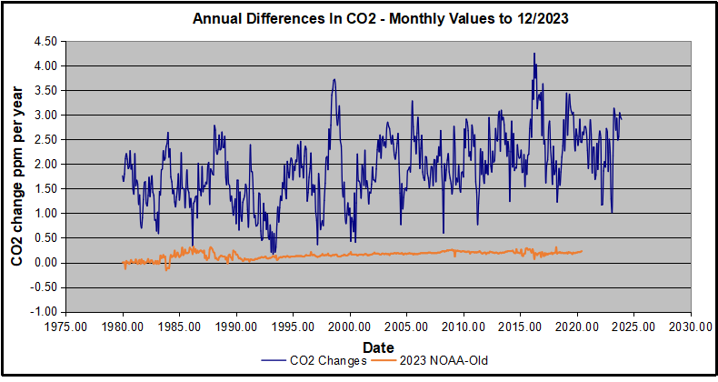
The blue line shows annual observed differences in monthly values year over year, e.g. June 2020 minus June 2019 etc.  The first 12 months (1979) provide the observed starting values from which differentials are calculated.  The orange line shows those CO2 values changed slightly in the 2020 dataset vs. the 2014 dataset, on average +0.035 ppm.  But there is no pattern or trend added, and deviations vary randomly between + and -.  So last year I took the 2020 dataset to replace the older one for updating the analysis.

Now I find the NOAA dataset starting in 2021 has almost completely new values due to a method shift in February 2021, requiring a recalibration of all previous measurements.  The new picture of ΔCO2 is graphed below.

The method shift is reported at a NOAA Global Monitoring Laboratory webpage, Carbon Dioxide (CO2) WMO Scale, with a justification for the difference between X2007 results and the new results from X2019 now in force.  The orange line shows that the shift has resulted in higher values, especially early on and a general slightly increasing trend over time.  However, these are small variations at the decimal level on values 340 and above.  Further, the graph shows that yearly differentials month by month are virtually the same as before.  Thus I redid the analysis with the new values.

Global Temperature Anomalies (ΔTemp)

The other time series was the record of global temperature anomalies according to RSS. The current RSS dataset is not at all the same as the past.

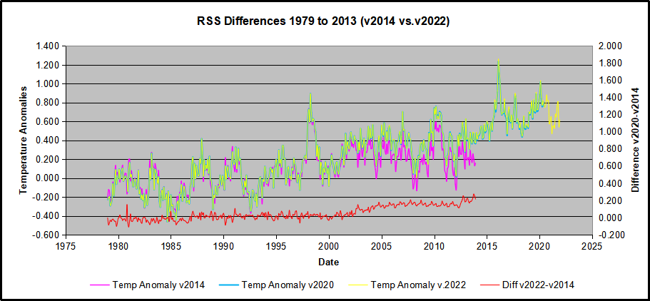
Here we see some seriously unsettling science at work.  The purple line is RSS in 2014, and the blue is RSS as of 2020.  Some further increases appear in the gold 2022 rss dataset. The red line shows alterations from the old to the new.  There is a slight cooling of the data in the beginning years, then the three versions mostly match until 1997, when systematic warming enters the record.  From 1997/5 to 2003/12 the average anomaly increases by 0.04C.  After 2004/1 to 2012/8 the average increase is 0.15C.  At the end from 2012/9 to 2013/12, the average anomaly was higher by 0.21. The 2022 version added slight warming over 2020 values.

RSS continues that accelerated warming to the present, but it cannot be trusted.  And who knows what the numbers will be a few years down the line?  As Dr. Ole Humlum said some years ago (regarding Gistemp): “It should however be noted, that a temperature record which keeps on changing the past hardly can qualify as being correct.”

Given the above manipulations, I went instead to the other satellite dataset UAH version 6. UAH has also made a shift by changing its baseline from 1981-2010 to 1991-2020.  This resulted in systematically reducing the anomaly values, but did not alter the pattern of variation over time.  For comparison, here are the two records with measurements through December 2023.

Comparing UAH temperature anomalies to NOAA CO2 changes.

Here are UAH temperature anomalies compared to CO2 monthly changes year over year.

Changes in monthly CO2 synchronize with temperature fluctuations, which for UAH are anomalies now referenced to the 1991-2020 period.  As stated above, CO2 differentials are calculated for the present month by subtracting the value for the same month in the previous year (for example June 2022 minus June 2021).   Temp anomalies are calculated by comparing the present month with the baseline month.

The final proof that CO2 follows temperature due to stimulation of natural CO2 reservoirs is demonstrated by the ability to calculate CO2 levels since 1979 with a simple mathematical formula:

For each subsequent year, the co2 level for each month was generated

CO2  this month this year = a + b × Temp this month this year  + CO2 this month last year

Jeremy used Python to estimate a and b, but I used his spreadsheet to guess values that place for comparison the observed and calculated CO2 levels on top of each other.

In the chart calculated CO2 levels correlate with observed CO2 levels at 0.9986 out of 1.0000.  This mathematical generation of CO2 atmospheric levels is only possible if they are driven by temperature-dependent natural sources, and not by human emissions which are small in comparison, rise steadily and monotonically.

Comment:  UAH dataset reported a sharp warming spike starting mid year, with causes speculated but not proven.  In any case, that surprising peak has not yet driven CO2 higher, though it might,  but only if it persists despite the likely cooling already under way.

Previous Post:  What Causes Rising Atmospheric CO2?

nasa_carbon_cycle_2008-1

This post is prompted by a recent exchange with those reasserting the “consensus” view attributing all additional atmospheric CO2 to humans burning fossil fuels.

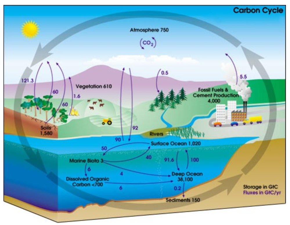
The IPCC doctrine which has long been promoted goes as follows. We have a number over here for monthly fossil fuel CO2 emissions, and a number over there for monthly atmospheric CO2. We don’t have good numbers for the rest of it-oceans, soils, biosphere–though rough estimates are orders of magnitude higher, dwarfing human CO2.  So we ignore nature and assume it is always a sink, explaining the difference between the two numbers we do have. Easy peasy, science settled.

What about the fact that nature continues to absorb about half of human emissions, even while FF CO2 increased by 60% over the last 2 decades? What about the fact that in 2020 FF CO2 declined significantly with no discernable impact on rising atmospheric CO2?

These and other issues are raised by Murray Salby and others who conclude that it is not that simple, and the science is not settled. And so these dissenters must be cancelled lest the narrative be weakened.

The non-IPCC paradigm is that atmospheric CO2 levels are a function of two very different fluxes. FF CO2 changes rapidly and increases steadily, while Natural CO2 changes slowly over time, and fluctuates up and down from temperature changes. The implications are that human CO2 is a simple addition, while natural CO2 comes from the integral of previous fluctuations.  Jeremy Shiers has a series of posts at his blog clarifying this paradigm. See Increasing CO2 Raises Global Temperature Or Does Increasing Temperature Raise CO2 Excerpts in italics with my bolds.

The following graph which shows the change in CO2 levels (rather than the levels directly) makes this much clearer.

Note the vertical scale refers to the first differential of the CO2 level not the level itself. The graph depicts that change rate in ppm per year.

There are big swings in the amount of CO2 emitted. Taking the mean as 1.6 ppmv/year (at a guess) there are +/- swings of around 1.2 nearly +/- 100%.

And, surprise surprise, the change in net emissions of CO2 is very strongly correlated with changes in global temperature.

This clearly indicates the net amount of CO2 emitted in any one year is directly linked to global mean temperature in that year.

For any given year the amount of CO2 in the atmosphere will be the sum of

  • all the net annual emissions of CO2
  • in all previous years.

For each year the net annual emission of CO2 is proportional to the annual global mean temperature.

This means the amount of CO2 in the atmosphere will be related to the sum of temperatures in previous years.

So CO2 levels are not directly related to the current temperature but the integral of temperature over previous years.

The following graph again shows observed levels of CO2 and global temperatures but also has calculated levels of CO2 based on sum of previous years temperatures (dotted blue line).

Summary:

The massive fluxes from natural sources dominate the flow of CO2 through the atmosphere.  Human CO2 from burning fossil fuels is around 4% of the annual addition from all sources. Even if rising CO2 could cause rising temperatures (no evidence, only claims), reducing our emissions would have little impact.

Atmospheric CO2 Math

Ins: 4% human, 96% natural
Outs: 0% human, 98% natural.
Atmospheric storage difference: +2%
(so that: Ins = Outs + Atmospheric storage difference)

Balance = Atmospheric storage difference: 2%, of which,
Humans: 2% X 4% = 0.08%
Nature: 2% X 96 % = 1.92%

Ratio Natural:Human =1.92% : 0.08% = 24 : 1

Resources
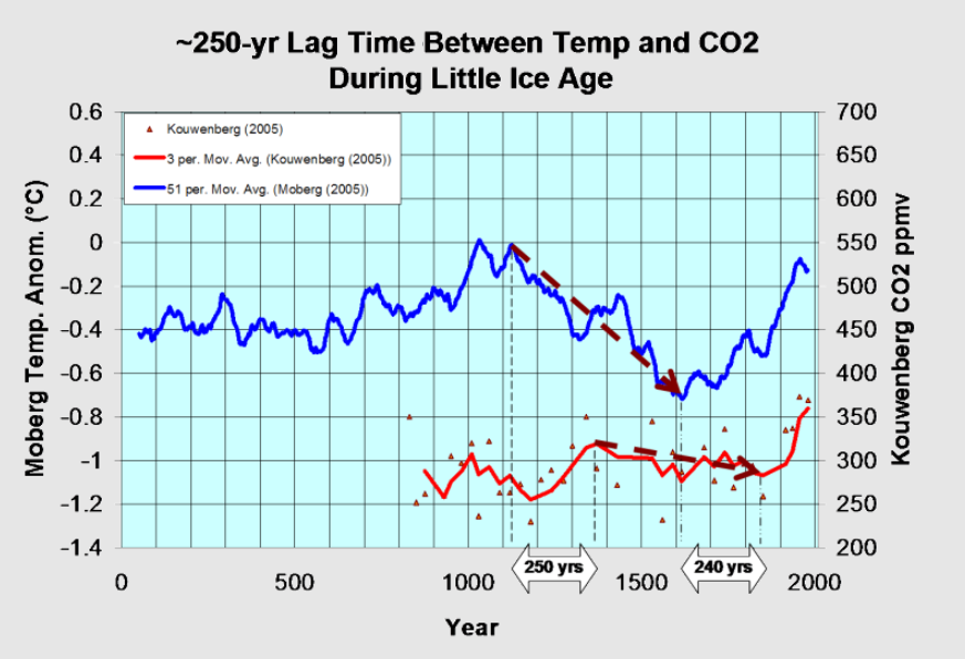
For a possible explanation of natural warming and CO2 emissions see Little Ice Age Warming Recovery May be Over
Resources:

CO2 Fluxes, Sources and Sinks

Who to Blame for Rising CO2?

Fearless Physics from Dr. Salby

Unsettled Science: How Sun’s Fluxes Affect Our Climate

John Green writes at American Thinker Why are we studying the sun, if the science is settled? Excerpts in italics with my bolds and added images.

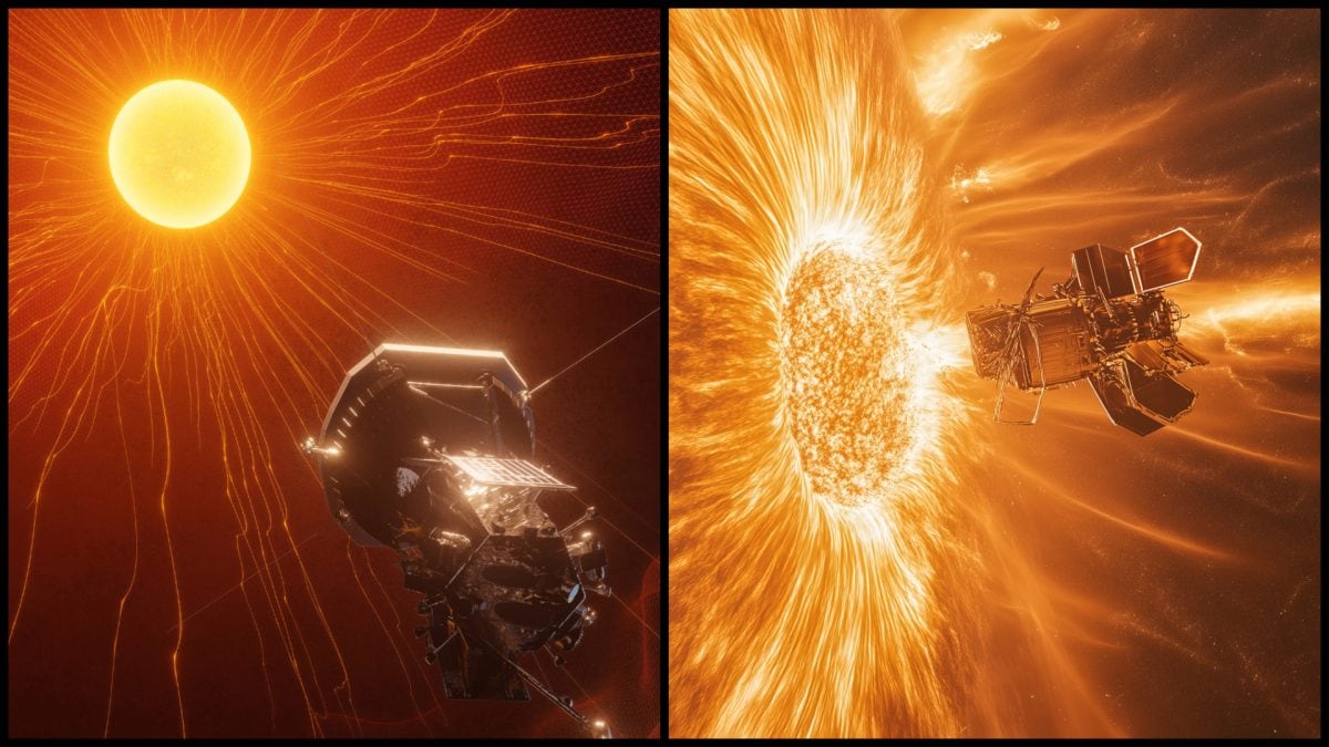
NASA’s Parker solar probe just completed one of its primary multi-year mission objectives, with the closest ever approach to the Sun. On Christmas Eve, the probe flew through the Sun’s corona at a blistering (literally and figuratively) 430,000 mph. For aircraft buffs, that’s Mach 560 — fast enough to circle the earth in about 3 minutes!

NASA’s Closest Approach to the Sun’s Fiery Surface Achieved by Parker Probe

A faint signal from Parker indicates that it survived its scorching flyby, and scientists are expecting it to download a treasure trove of data later this month. It turns out there’s a lot the guys with the PhDs don’t understand about the sun. As NASA states:

The NASA Parker Solar Probe mission is a mission designed to help humanity better understand the Sun, where changing conditions can propagate out into the solar system, affecting Earth and other worlds. As such, the primary goals are to examine the acceleration of solar wind through the movement of heat and energy in the Sun’s corona in addition to study solar energetic particles.

They’re hoping data collected while flying through the Sun’s corona will provide a few answers and make it a bit more predictable.

I confess I’m just a lowly engineer, and many of the mysteries they’re trying to unravel are well beyond my college physics courses. But reading about the Parker probe got me wondering: Doesn’t the Sun have something to do with our weather? I mean it’s warm on sunny days, and plants grow better when the earth’s surface is the closest to the Sun.

Those observations may sound obtuse, but they’re no more obtuse than “experts” saying that “climate science is settled” — when they don’t understand how the freaking Sun works! (Looking at you “Science Guy” Bill Nye.)

The science can only be settled when the smart guys understand all the factors that affect our climate — and how they interact — well enough to predict outcomes. The Sun imparts about 342 watts of energy on every square meter of the earth’s surface (according to NASA). That’s the equivalent of 44 million average electric power plants (700 times what the world has) — yet we don’t understand its fluctuations.

That’s a rather big unpredictable factor for this supposedly “settled science” — no?

One can only conclude that when highly educated people — who should know better — claim climate science is settled, they’re lying. Perhaps that’s why multiple predictions that the polar bears would be extinct and New York would be underwater by now have all been wrong. It might also explain why the greenies avoid discussion of ice ages and interglacial periods when assuring us that our cars are delivering planetary doom – while their private jets are perfectly fine.

Given what little we know about the Sun, the anthropogenic climate change “experts” are either:

  • Ignorant men, succumbing to irrational fears — placing superstition above science, or
  • Evil men — profiting by scaring us into irrational behavior.

We should keep that in mind when they insist that we halt progress, live in destitution, and scare our children that apocalypse is imminent. Our only rational response is to ignore them … and cut off their funding.

Yes, IPCC, Our Climate Responds to Our Sun

John Gideon Hartnett writes at Spectator Australia The sun is in control of our oceans. Text is from John Ray at his blog, excerpts in italics with my bolds and added images.

In recent years, there has been observed an increase in ocean temperature. Those who adhere to the Climate Change version of events say that the oceans are getting warmer because of trapped carbon dioxide (CO2) in the atmosphere causing a massive greenhouse effect leading to boiling oceans.

Well, anyone who has a brain knows that the oceans are not boiling, but let’s assume that is just hyperbole. When actual research – when actual measurements were taken – reality turns out to be the exact opposite.

New research shows that the temperature of our oceans are controlled by incident radiation from the Sun. Who would have guessed?

And as a consequence of the oceans warming, dissolved carbon dioxide gas is released due to reduced is solubility in ocean water. This means the warming of the oceans would lead (or cause) an increase in CO2 concentration in the atmosphere.  One of the researchers in the study wrote on X.com:

A decrease in cloud cover and albedo means more short wavelength (SW) solar radiation reaches the oceans. Albedo is the reflectivity of the Earth. Lower albedo means more sunlight reaching the land and oceans and more warming by the Sun.

Figure 8. Comparison between observed global temperature anomalies and CERES-reported changes in the Earth’s absorbed solar flux. The two data series representing 13-month running means are highly correlated with the absorbed SW flux explaining 78% of the temperature variation (R2 = 0.78). The global temperature lags the absorbed solar radiation between 0 and 9 months, which indicates that climate change in the 21st Century was driven by solar forcing.

I mean to say that this is so obvious. The Sun heats Earth’s surface of which 71% is covered by the oceans! Basic physics!

The energy from the Sun powers all life on the planet and causes all Earth changes. Every second, the Earth receives the equivalent energy of 42 megatons of TNT in radiation from the Sun. That cannot be ignored. 

Climate Change, the ideological movement which I prefer to call a cult, views all evidence through the lens of their religious belief that the Earth is warmed by human activity. That activity releases carbon dioxide gas, which has been observed to be increasing. Their belief is that CO2 traps heat in a giant greenhouse effect. That is the dogma anyway. And I must add, we all are the carbon they want to eliminate.

But how much of that observed increase in CO2 is actually from natural causes and not from human activity? At least 94 per cent is. This new evidence now suggests it could be even more than that.

If the oceans emit CO2 gas following changes in the water temperature, which this research shows is due to the amount (flux) of solar radiation reaching the surface, then more CO2 comes from natural causes.

It is basic physics that as you heat water the dissolved gases are released due to a decrease in gas solubility. This means as the solar flux increases CO2 gas is released from the warmer ocean water.

Thus an ocean temperature increase leads to an increase in CO2 in the atmosphere, and not the other way around.

Space weather impacts the ionosphere in this animation. Credits: NASA/GSFC/CIL/Krystofer Kim

Ocean Leads Cooling UAH December 2024

The post below updates the UAH record of air temperatures over land and ocean. Each month and year exposes again the growing disconnect between the real world and the Zero Carbon zealots.  It is as though the anti-hydrocarbon band wagon hopes to drown out the data contradicting their justification for the Great Energy Transition.  Yes, there was warming from an El Nino buildup coincidental with North Atlantic warming, but no basis to blame it on CO2.  

As an overview consider how recent rapid cooling  completely overcame the warming from the last 3 El Ninos (1998, 2010 and 2016).  The UAH record shows that the effects of the last one were gone as of April 2021, again in November 2021, and in February and June 2022  At year end 2022 and continuing into 2023 global temp anomaly matched or went lower than average since 1995, an ENSO neutral year. (UAH baseline is now 1991-2020). Now we have had an usual El Nino warming spike of uncertain cause, unrelated to steadily rising CO2 and now dropping steadily.

For reference I added an overlay of CO2 annual concentrations as measured at Mauna Loa.  While temperatures fluctuated up and down ending flat, CO2 went up steadily by ~60 ppm, a 15% increase.

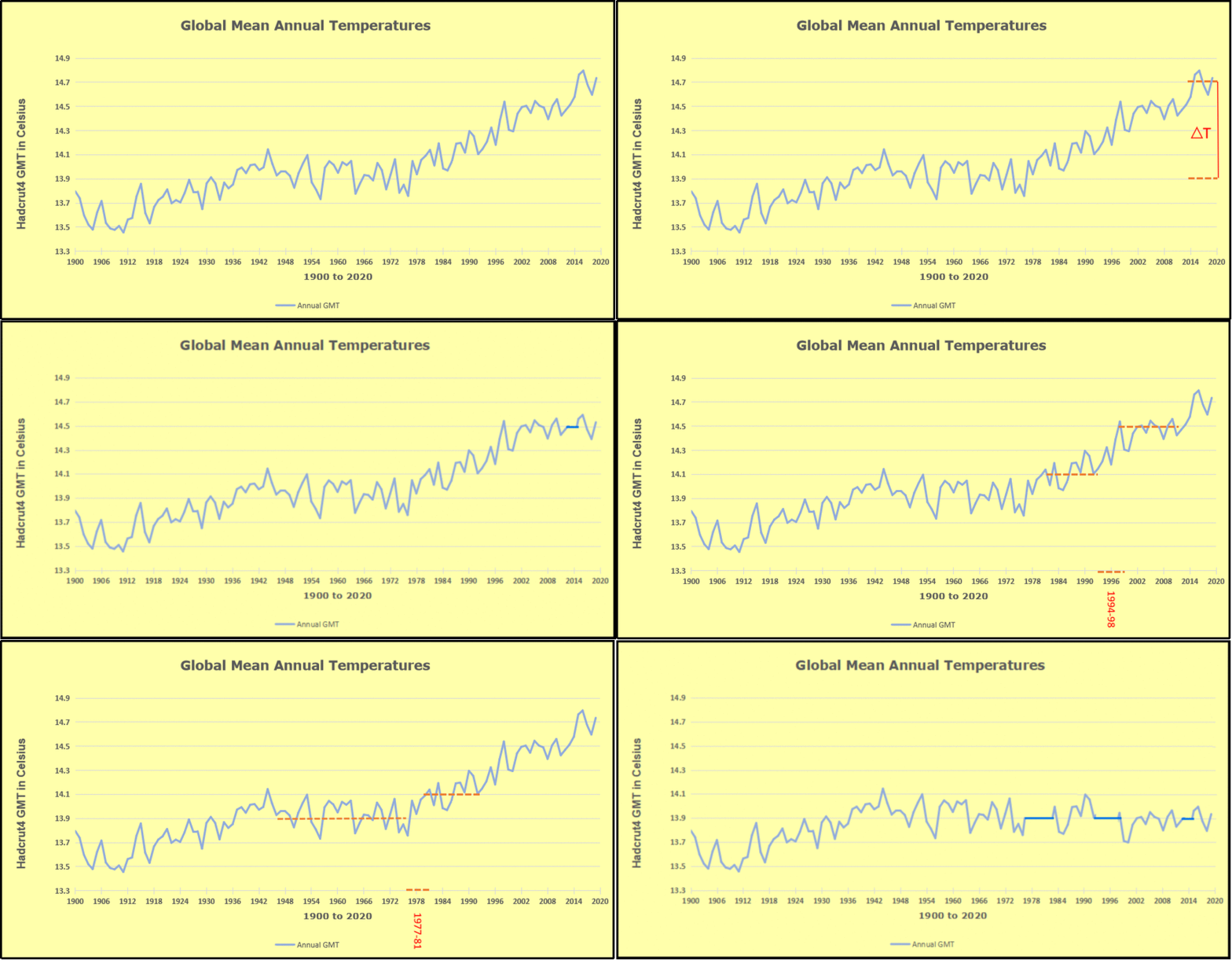
Furthermore, going back to previous warmings prior to the satellite record shows that the entire rise of 0.8C since 1947 is due to oceanic, not human activity.

gmt-warming-events

The animation is an update of a previous analysis from Dr. Murry Salby.  These graphs use Hadcrut4 and include the 2016 El Nino warming event.  The exhibit shows since 1947 GMT warmed by 0.8 C, from 13.9 to 14.7, as estimated by Hadcrut4.  This resulted from three natural warming events involving ocean cycles. The most recent rise 2013-16 lifted temperatures by 0.2C.  Previously the 1997-98 El Nino produced a plateau increase of 0.4C.  Before that, a rise from 1977-81 added 0.2C to start the warming since 1947.

Importantly, the theory of human-caused global warming asserts that increasing CO2 in the atmosphere changes the baseline and causes systemic warming in our climate.  On the contrary, all of the warming since 1947 was episodic, coming from three brief events associated with oceanic cycles. And now in 2024 we have seen an amazing episode with a temperature spike driven by ocean air warming in all regions, along with rising NH land temperatures, now dropping below its peak.

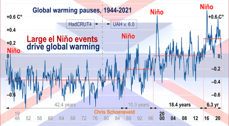
Chris Schoeneveld has produced a similar graph to the animation above, with a temperature series combining HadCRUT4 and UAH6. H/T WUWT

image-8


mc_wh_gas_web20210423124932

See Also Worst Threat: Greenhouse Gas or Quiet Sun?

December 2024 Ocean Leads Global Cooling banner-blog

With apologies to Paul Revere, this post is on the lookout for cooler weather with an eye on both the Land and the Sea.  While you heard a lot about 2020-21 temperatures matching 2016 as the highest ever, that spin ignores how fast the cooling set in.  The UAH data analyzed below shows that warming from the last El Nino had fully dissipated with chilly temperatures in all regions. After a warming blip in 2022, land and ocean temps dropped again with 2023 starting below the mean since 1995.  Spring and Summer 2023 saw a series of warmings, continuing into October, followed by cooling in November and December.

UAH has updated their TLT (temperatures in lower troposphere) dataset for December 2024. Due to one satellite drifting more than can be corrected, the dataset has been recalibrated and retitled as version 6.1 Graphs here contain this updated 6.1 data.  Posts on their reading of ocean air temps this month are ahead of the update from HadSST4.  I posted recently on SSTs Ocean Remains Cooler November 2024. These posts have a separate graph of land air temps because the comparisons and contrasts are interesting as we contemplate possible cooling in coming months and years.

Sometimes air temps over land diverge from ocean air changes. In July 2024 all oceans were unchanged except for Tropical warming, while all land regions rose slightly. In August we saw a warming leap in SH land, slight Land cooling elsewhere, a dip in Tropical Ocean temp and slightly elsewhere.  September showed a dramatic drop in SH land, overcome by a greater NH land increase. In October, ocean and land temps in both NH and Tropics dropped, pulling the global anomaly down. Now in November and December there was cooling everywhere, except only SH and Tropics land temps.

Note:  UAH has shifted their baseline from 1981-2010 to 1991-2020 beginning with January 2021.   v6.1 data was recalibrated also starting with 2021. In the charts below, the trends and fluctuations remain the same but the anomaly values changed with the baseline reference shift.

Presently sea surface temperatures (SST) are the best available indicator of heat content gained or lost from earth’s climate system.  Enthalpy is the thermodynamic term for total heat content in a system, and humidity differences in air parcels affect enthalpy.  Measuring water temperature directly avoids distorted impressions from air measurements.  In addition, ocean covers 71% of the planet surface and thus dominates surface temperature estimates.  Eventually we will likely have reliable means of recording water temperatures at depth.

Recently, Dr. Ole Humlum reported from his research that air temperatures lag 2-3 months behind changes in SST.  Thus cooling oceans portend cooling land air temperatures to follow.  He also observed that changes in CO2 atmospheric concentrations lag behind SST by 11-12 months.  This latter point is addressed in a previous post Who to Blame for Rising CO2?

After a change in priorities, updates are now exclusive to HadSST4.  For comparison we can also look at lower troposphere temperatures (TLT) from UAHv6.1 which are now posted for December.  The temperature record is derived from microwave sounding units (MSU) on board satellites like the one pictured above. Recently there was a change in UAH processing of satellite drift corrections, including dropping one platform which can no longer be corrected. The graphs below are taken from the revised and current dataset.

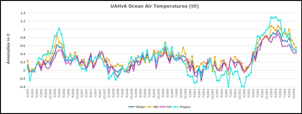
The UAH dataset includes temperature results for air above the oceans, and thus should be most comparable to the SSTs. There is the additional feature that ocean air temps avoid Urban Heat Islands (UHI).  The graph below shows monthly anomalies for ocean air temps since January 2015.

In 2021-22, SH and NH showed spikes up and down while the Tropics cooled dramatically, with some ups and downs, but hitting a new low in January 2023. At that point all regions were more or less in negative territory. 

After sharp cooling everywhere in January 2023, there was a remarkable spiking of Tropical ocean temps from -0.5C up to + 1.2C in January 2024.  The rise was matched by other regions in 2024, such that the Global anomaly peaked at 0.95C in May, Since then the Tropics and the Global anomaly have cooled down to 0.5C, as well as SH dropping down to 0.4C in December.

Land Air Temperatures Tracking in Seesaw Pattern

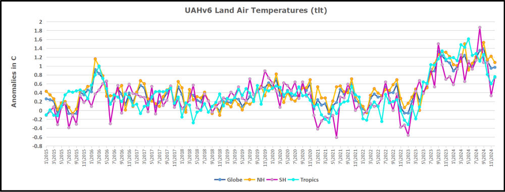
We sometimes overlook that in climate temperature records, while the oceans are measured directly with SSTs, land temps are measured only indirectly.  The land temperature records at surface stations sample air temps at 2 meters above ground.  UAH gives tlt anomalies for air over land separately from ocean air temps.  The graph updated for December is below.

Here we have fresh evidence of the greater volatility of the Land temperatures, along with extraordinary departures by SH land.  The seesaw pattern in Land temps is similar to ocean temps 2021-22, except that SH is the outlier, hitting bottom in January 2023. Then exceptionally SH goes from -0.6C up to 1.4C in September 2023 and 1.8C in  August 2024, with a large drop in between.  In November, SH and the Tropics pulled the Global Land anomaly further down despite a bump in NH land temps. December showed an upward rebound in SH and Tropics land temps, offset by a NH drop, leaving the Global land anomaly little changed.

The Bigger Picture UAH Global Since 1980

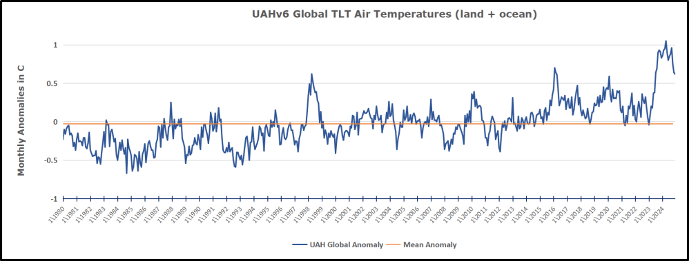
The chart shows monthly Global Land and Ocean anomalies starting 01/1980 to present.  The average monthly anomaly is -0.03, for this period of more than four decades.  The graph shows the 1998 El Nino after which the mean resumed, and again after the smaller 2010 event. The 2016 El Nino matched 1998 peak and in addition NH after effects lasted longer, followed by the NH warming 2019-20.   An upward bump in 2021 was reversed with temps having returned close to the mean as of 2/2022.  March and April brought warmer Global temps, later reversed

With the sharp drops in Nov., Dec. and January 2023 temps, there was no increase over 1980. Then in 2023 the buildup to the October/November peak exceeded the sharp April peak of the El Nino 1998 event. It also surpassed the February peak in 2016. In 2024 March and April took the Global anomaly to a new peak of 0.94C.  The cool down started with May dropping to 0.9C, and in June a further decline to 0.8C.  October went down to 0.7C,  November and December dropped to 0.6C. 

The graph reminds of another chart showing the abrupt ejection of humid air from Hunga Tonga eruption.

TLTs include mixing above the oceans and probably some influence from nearby more volatile land temps.  Clearly NH and Global land temps have been dropping in a seesaw pattern, nearly 1C lower than the 2016 peak.  Since the ocean has 1000 times the heat capacity as the atmosphere, that cooling is a significant driving force.  TLT measures started the recent cooling later than SSTs from HadSST4, but are now showing the same pattern. Despite the three El Ninos, their warming had not persisted prior to 2023, and without them it would probably have cooled since 1995.  Of course, the future has not yet been written.


Lacking Data, Climate Models Rely on Guesses

A recent question was posed on  Quora: Say there are merely 15 variables involved in predicting global climate change. Assume climatologists have mastered each variable to a near perfect accuracy of 95%. How accurate would a climate model built on this simplified system be?  Keith Minor has a PhD in organic chemistry, PhD in Geology, and PhD in Geology & Paleontology from The University of Texas at Austin.  He responded with the text posted below in italics with my bolds and added images.

I like the answers to this question, and Matthew stole my thunder on the climate models not being statistical models. If we take the question and it’s assumptions at face value, one unsolvable overriding problem, and a limit to developing an accurate climate model that is rarely ever addressed, is the sampling issue. Knowing 15 parameters to 99+% accuracy won’t solve this problem.

The modeling of the atmosphere is a boundary condition problem. No, I’m not talking about frontal boundaries. Thermodynamic systems are boundary condition problems, meaning that the evolution of a thermodynamic system is dependent not only on the conditions at t > 0 (is the system under adiabatic conditions, isothermal conditions, do these conditions change during the process, etc.?), but also on the initial conditions at t = 0 (sec, whatever). Knowing almost nothing about what even a fraction of a fraction of the molecules in the atmosphere are doing at t = 0 or at t > 0 is a huge problem to accurately predicting what the atmosphere will do in the near or far future. [See footnote at end on this issue.]

Edward Lorenz attempted to model the thermodynamic behavior of the atmosphere by using models that took into account twelve variables (instead of fifteen as posed by the questioner), and found (not surprisingly) that there was a large variability in the models. Seemingly inconsequential perturbations would lead to drastically different results, which diverged (euphemism for “got even worse”) the longer out in time the models were run (they still do). This presumably is the origin of Lorenz’s phrase “the butterfly effect”. He probably meant it to be taken more as an instructive hypothetical rather than a literal effect, as it is too often taken today. He was merely illustrating the sensitivity of the system to the values of the parameters, and not equating it to the probability of outcomes, chaos theory, etc., which is how the term has come to be known. This divergence over time is bad for climate models, which try to predict the climate decades from now. Just look at the divergence of hurricane “spaghetti” models, which operate on a multiple-week scale.

The sources of variability include:

♦  the inability of the models to handle water (the most important greenhouse gas in the atmosphere, not CO2) and processes related to it;
♦  e.g., models still can’t handle the formation and non-formation of clouds;
♦  the non-linearity of thermodynamic properties of matter (which seem to be an afterthought, especially in popular discussions regarding the roles that CO2 plays in the atmosphere and biosphere), and
♦  the always-present sampling problem.

While in theory it is possible to know what a statistically significant number of the air and water molecules are doing at any point in time (that would be a lot of atoms and molecules!), a statistically significant sample of air molecules is certainly not being sampled by releasing balloons twice a day from 90 some odd weather stations in the US and territories, plus the data from commercial aircraft, plus all of the weather data from around the World. Doubling this number wouldn’t help, i.e wouldn’t make any difference. Though there are some blind spots, such as northeast Texas that might benefit from having a radar in the area. So you have to weigh the cost of sampling more of the atmosphere versus the 0% increase in forecasting accuracy (within experimental error) that you would get by doing so.

I’ll go out on a limb and say that the NWS (National Weather Service) is actually doing pretty good job in their 5-day forecasts with the current data and technologies that they have (e.g., S-band radar), and the local meteorologists use their years of experience and judgment to refine the forecasts to their viewing areas. The old joke is that a meteorologist’s job is the one job where you can be wrong more than half the time and still keep your job, but everyone knows that they go to work most, if not all, days with one hand tied behind their back, and sometimes two! The forecasts are not that far off on average, and so meteorologists get my unconditional respect.

In spite of these daunting challenges, there are certainly a number of areas in weather forecasting that can be improved by increased sampling, especially on a local scale. For example, for severe weather outbreaks, the CASA project is being implemented using multiple, shorter range radars that can get multiple scan directions on nearby severe-warned cells simultaneously. This resolves the problem caused by the curvature of the Earth as well as other problems associated with detecting storm-scale features tens or hundreds of miles away from the radar. So high winds, hail, and tornadoes are weather events where increasing the local sampling density/rate might help improve both the models and forecasts.

Prof. Wurman at OU has been doing this for decades with his pioneering work with mobile radar (the so-called “DOW’s”). Let’s not leave out the other researchers who have also been doing this for decades. The strategy of collecting data on a storm from multiple directions at short distances, coupled with supercomputer capabilities, has been paying off for a number of years. As a recent example, Prof. Orf at UW Madison, with his simulation of the May 24th, 2011 El Reno, OK tornado (you’ve probably seen it on the Internet), has shed light on some of the “black box” aspects to how tornadoes form. [Video below is Leigh Orf 1.5 min segment for 2018 Blue Waters Symposium plenary session. This segment summarizes, in 90 seconds, some of the team’s accomplishments on the Blue Waters supercomputer over the past five years.]

Prof. Orf’s simulation is just that, and the resolution is around ~10 m (~33 feet), but it illustrates how increased targeted sampling can be effective in at least understanding the complex, thermodynamic processes occurring within a storm. Colleagues have argued that the small improvements in warning times in the last couple of decades are really due more to the heavy spotter presence these days rather than case studies of severe storms. That may be true. However, in test cases of the CASA system, it picked out the subtle boundaries along which the storms fired that did go unnoticed with the current network of radars. So I’m optimistic about increased targeted sampling for use in an early warning system.

These two examples bring up a related problem-too much data! As commented on by a local meteorologist at a TESSA meeting, one of the issues with CASA that will have to be resolved is how to handle/process the tremendous amounts of data that will be generated during a severe weather outbreak. This is different from a research project where you can take your data back to the “lab”. In a real-time system, such as CASA, you need to have the ability to process the volumes of data rapidly so a meteorologist can quickly make a decision and get that life-saving info to the public. This data volume issue may be less of a problem for those using the data to develop climate models.

So back to the Quora question, with regard to a cost-effective (cost-effect is the operational term) climate model or models (say an ensemble model) that would “verify” say 50 years from now, the sampling issue is ever present, and likely cost-prohibitive at the level needed to make the sampling statistically significant. And will the climatologist be around in 50 years to be “hoisted with their own petard” when the climate model is proven to be wrong? The absence of accountability is the other problem with these long-range models into which many put so much faith.

But don’t stop using or trying to develop better climate models. Just be aware of what variables they include, how well they handle the parameters, and what their limitations are. How accurate would a climate model built on this simplified system [edit: of 15 well-defined variables (to 95% confidence level)] be? Not very!

My Comment

As Dr. Minor explains, powerful modern computers can process detailed observation data to simulate and forecast storm activity.  There are more such tools for preparing and adapting to extreme weather events which are normal in our climate system and beyond our control.  He also explains why long-range global climate models presently have major limitations for use by policymakers.

Footnote Regarding Initial Conditions Problem

What About the Double Pendulum?

Trajectories of a double pendulum

comment by tom0mason at alerted me to the science demonstrated by the double compound pendulum, that is, a second pendulum attached to the ball of the first one. It consists entirely of two simple objects functioning as pendulums, only now each is influenced by the behavior of the other.

Lo and behold, you observe that a double pendulum in motion produces chaotic behavior. In a remarkable achievement, complex equations have been developed that can and do predict the positions of the two balls over time, so in fact the movements are not truly chaotic, but with considerable effort can be determined. The equations and descriptions are at Wikipedia Double Pendulum

Long exposure of double pendulum exhibiting chaotic motion (tracked with an LED)

But here is the kicker, as described in tomomason’s comment:

If you arrive to observe the double pendulum at an arbitrary time after the motion has started from an unknown condition (unknown height, initial force, etc) you will be very taxed mathematically to predict where in space the pendulum will move to next, on a second to second basis. Indeed it would take considerable time and many iterative calculations (preferably on a super-computer) to be able to perform this feat. And all this on a very basic system of known elementary mechanics.

Our Chaotic Climate System


Ocean Remains Cooler November 2024

The best context for understanding decadal temperature changes comes from the world’s sea surface temperatures (SST), for several reasons:

  • The ocean covers 71% of the globe and drives average temperatures;
  • SSTs have a constant water content, (unlike air temperatures), so give a better reading of heat content variations;
  • Major El Ninos have been the dominant climate feature in recent years.

HadSST is generally regarded as the best of the global SST data sets, and so the temperature story here comes from that source. Previously I used HadSST3 for these reports, but Hadley Centre has made HadSST4 the priority, and v.3 will no longer be updated.  HadSST4 is the same as v.3, except that the older data from ship water intake was re-estimated to be generally lower temperatures than shown in v.3.  The effect is that v.4 has lower average anomalies for the baseline period 1961-1990, thereby showing higher current anomalies than v.3. This analysis concerns more recent time periods and depends on very similar differentials as those from v.3 despite higher absolute anomaly values in v.4.  More on what distinguishes HadSST3 and 4 from other SST products at the end. The user guide for HadSST4 is here.

The Current Context

The chart below shows SST monthly anomalies as reported in HadSST4 starting in 2015 through November 2024.  A global cooling pattern is seen clearly in the Tropics since its peak in 2016, joined by NH and SH cycling downward since 2016, followed by rising temperatures in 2023 and 2024.

Note that in 2015-2016 the Tropics and SH peaked in between two summer NH spikes.  That pattern repeated in 2019-2020 with a lesser Tropics peak and SH bump, but with higher NH spikes. By end of 2020, cooler SSTs in all regions took the Global anomaly well below the mean for this period.  A small warming was driven by NH summer peaks in 2021-22, but offset by cooling in SH and the tropics, By January 2023 the global anomaly was again below the mean.

Now in 2023-24 came an event resembling 2015-16 with a Tropical spike and two NH spikes alongside, all higher than 2015-16. There was also a coinciding rise in SH, and the Global anomaly was pulled up to 1.1°C last year, ~0.3° higher than the 2015 peak.  Then NH started down autumn 2023, followed by Tropics and SH descending 2024 to the present. After 10 months of cooling in SH and the Tropics, the Global anomaly was back down, led by NH cooling the last 3 months from its peak in August.

Comment:

The climatists have seized on this unusual warming as proof their Zero Carbon agenda is needed, without addressing how impossible it would be for CO2 warming the air to raise ocean temperatures.  It is the ocean that warms the air, not the other way around.  Recently Steven Koonin had this to say about the phonomenon confirmed in the graph above:

El Nino is a phenomenon in the climate system that happens once every four or five years.  Heat builds up in the equatorial Pacific to the west of Indonesia and so on.  Then when enough of it builds up it surges across the Pacific and changes the currents and the winds.  As it surges toward South America it was discovered and named in the 19th century  It iswell understood at this point that the phenomenon has nothing to do with CO2.

Now people talk about changes in that phenomena as a result of CO2 but it’s there in the climate system already and when it happens it influences weather all over the world.   We feel it when it gets rainier in Southern California for example.  So for the last 3 years we have been in the opposite of an El Nino, a La Nina, part of the reason people think the West Coast has been in drought.

It has now shifted in the last months to an El Nino condition that warms the globe and is thought to contribute to this Spike we have seen. But there are other contributions as well.  One of the most surprising ones is that back in January of 2022 an enormous underwater volcano went off in Tonga and it put up a lot of water vapor into the upper atmosphere. It increased the upper atmosphere of water vapor by about 10 percent, and that’s a warming effect, and it may be that is contributing to why the spike is so high.

A longer view of SSTs

Open image in new tab to enlarge.

The graph above is noisy, but the density is needed to see the seasonal patterns in the oceanic fluctuations.  Previous posts focused on the rise and fall of the last El Nino starting in 2015.  This post adds a longer view, encompassing the significant 1998 El Nino and since.  The color schemes are retained for Global, Tropics, NH and SH anomalies.  Despite the longer time frame, I have kept the monthly data (rather than yearly averages) because of interesting shifts between January and July. 1995 is a reasonable (ENSO neutral) starting point prior to the first El Nino. 

The sharp Tropical rise peaking in 1998 is dominant in the record, starting Jan. ’97 to pull up SSTs uniformly before returning to the same level Jan. ’99. There were strong cool periods before and after the 1998 El Nino event. Then SSTs in all regions returned to the mean in 2001-2. 

SSTS fluctuate around the mean until 2007, when another, smaller ENSO event occurs. There is cooling 2007-8,  a lower peak warming in 2009-10, following by cooling in 2011-12.  Again SSTs are average 2013-14.

Now a different pattern appears.  The Tropics cooled sharply to Jan 11, then rise steadily for 4 years to Jan 15, at which point the most recent major El Nino takes off.  But this time in contrast to ’97-’99, the Northern Hemisphere produces peaks every summer pulling up the Global average.  In fact, these NH peaks appear every July starting in 2003, growing stronger to produce 3 massive highs in 2014, 15 and 16.  NH July 2017 was only slightly lower, and a fifth NH peak still lower in Sept. 2018.

The highest summer NH peaks came in 2019 and 2020, only this time the Tropics and SH were offsetting rather adding to the warming. (Note: these are high anomalies on top of the highest absolute temps in the NH.)  Since 2014 SH has played a moderating role, offsetting the NH warming pulses. After September 2020 temps dropped off down until February 2021.  In 2021-22 there were again summer NH spikes, but in 2022 moderated first by cooling Tropics and SH SSTs, then in October to January 2023 by deeper cooling in NH and Tropics.  

Then in 2023 the Tropics flipped from below to well above average, while NH produced a summer peak extending into September higher than any previous year.  Despite El Nino driving the Tropics January 2024 anomaly higher than 1998 and 2016 peaks, following months cooled in all regions, and the Tropics continued cooling in April, May and June along with SH dropping.  After July and August NH warming again pulled the global anomaly higher, September and October resumed cooling in all regions.

What to make of all this? The patterns suggest that in addition to El Ninos in the Pacific driving the Tropic SSTs, something else is going on in the NH.  The obvious culprit is the North Atlantic, since I have seen this sort of pulsing before.  After reading some papers by David Dilley, I confirmed his observation of Atlantic pulses into the Arctic every 8 to 10 years.

Contemporary AMO Observations

Through January 2023 I depended on the Kaplan AMO Index (not smoothed, not detrended) for N. Atlantic observations. But it is no longer being updated, and NOAA says they don’t know its future.  So I find that ERSSTv5 AMO dataset has current data.  It differs from Kaplan, which reported average absolute temps measured in N. Atlantic.  “ERSST5 AMO  follows Trenberth and Shea (2006) proposal to use the NA region EQ-60°N, 0°-80°W and subtract the global rise of SST 60°S-60°N to obtain a measure of the internal variability, arguing that the effect of external forcing on the North Atlantic should be similar to the effect on the other oceans.”  So the values represent sst anomaly differences between the N. Atlantic and the Global ocean.

The chart above confirms what Kaplan also showed.  As August is the hottest month for the N. Atlantic, its variability, high and low, drives the annual results for this basin.  Note also the peaks in 2010, lows after 2014, and a rise in 2021. Then in 2023 the peak was holding at 1.4C before declining.  An annual chart below is informative:

Note the difference between blue/green years, beige/brown, and purple/red years.  2010, 2021, 2022 all peaked strongly in August or September.  1998 and 2007 were mildly warm.  2016 and 2018 were matching or cooler than the global average.  2023 started out slightly warm, then rose steadily to an  extraordinary peak in July.  August to October were only slightly lower, but by December cooled by ~0.4C.

Then in 2024 the AMO anomaly started higher than any previous year, then leveled off for two months declining slightly into April.  Remarkably, May showed an upward leap putting this on a higher track than 2023, and rising slightly higher in June.  In July, August and September 2024 the anomaly declined, and despite a small rise in October, is now lower than the peak reached in 2023.

The pattern suggests the ocean may be demonstrating a stairstep pattern like that we have also seen in HadCRUT4. 

The purple line is the average anomaly 1980-1996 inclusive, value 0.18.  The orange line the average 1980-202404, value 0.39, also for the period 1997-2012. The red line is 2013-202409, value 0.69. As noted above, these rising stages are driven by the combined warming in the Tropics and NH, including both Pacific and Atlantic basins.

See Also:

2024 El Nino Collapsing

Curiosity:  Solar Coincidence?

The news about our current solar cycle 25 is that the solar activity is hitting peak numbers now and higher  than expected 1-2 years in the future.  As livescience put it:  Solar maximum could hit us harder and sooner than we thought. How dangerous will the sun’s chaotic peak be?  Some charts from spaceweatherlive look familar to these sea surface temperature charts.

Summary

The oceans are driving the warming this century.  SSTs took a step up with the 1998 El Nino and have stayed there with help from the North Atlantic, and more recently the Pacific northern “Blob.”  The ocean surfaces are releasing a lot of energy, warming the air, but eventually will have a cooling effect.  The decline after 1937 was rapid by comparison, so one wonders: How long can the oceans keep this up? And is the sun adding forcing to this process?

Space weather impacts the ionosphere in this animation. Credits: NASA/GSFC/CIL/Krystofer Kim

Footnote: Why Rely on HadSST4

HadSST is distinguished from other SST products because HadCRU (Hadley Climatic Research Unit) does not engage in SST interpolation, i.e. infilling estimated anomalies into grid cells lacking sufficient sampling in a given month. From reading the documentation and from queries to Met Office, this is their procedure.

HadSST4 imports data from gridcells containing ocean, excluding land cells. From past records, they have calculated daily and monthly average readings for each grid cell for the period 1961 to 1990. Those temperatures form the baseline from which anomalies are calculated.

In a given month, each gridcell with sufficient sampling is averaged for the month and then the baseline value for that cell and that month is subtracted, resulting in the monthly anomaly for that cell. All cells with monthly anomalies are averaged to produce global, hemispheric and tropical anomalies for the month, based on the cells in those locations. For example, Tropics averages include ocean grid cells lying between latitudes 20N and 20S.

Gridcells lacking sufficient sampling that month are left out of the averaging, and the uncertainty from such missing data is estimated. IMO that is more reasonable than inventing data to infill. And it seems that the Global Drifter Array displayed in the top image is providing more uniform coverage of the oceans than in the past.

uss-pearl-harbor-deploys-global-drifter-buoys-in-pacific-ocean

USS Pearl Harbor deploys Global Drifter Buoys in Pacific Ocean


2024 Natural Climate Factors: Snow

Previously I posted an explanation by Dr. Judah Cohen regarding a correlation between autumn Siberian snow cover and the following winter conditions, not only in the Arctic but extending across the Northern Hemisphere. More recently, in looking into Climate Model Upgraded: INMCM5, I noticed some of the scientists were also involved in confirming the importance of snow cover for climate forecasting. Since the poles function as the primary vents for global cooling, what happens in the Arctic in no way stays in the Arctic. This post explores data suggesting changes in snow cover drive some climate changes.

The Snow Cover Climate Factor

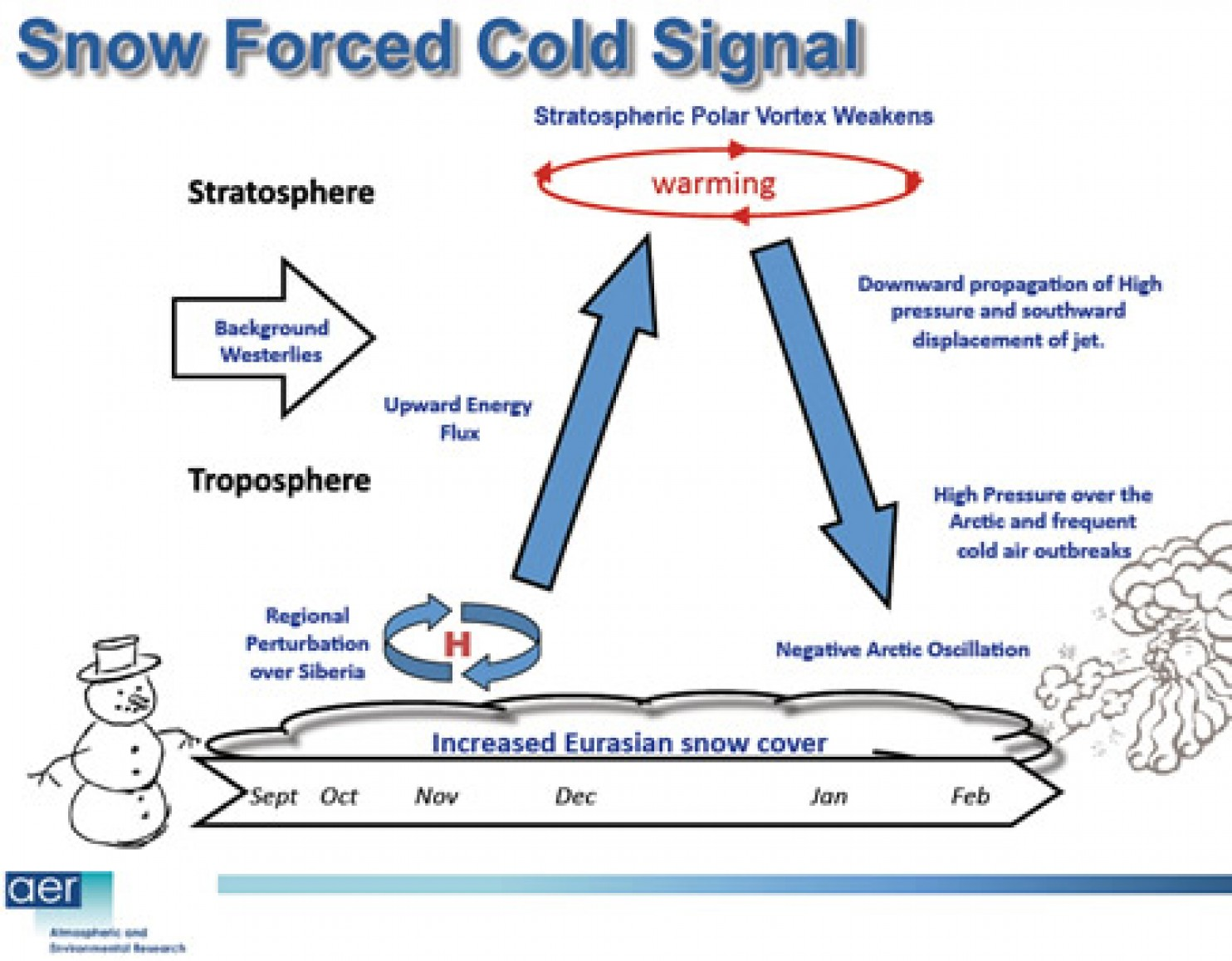
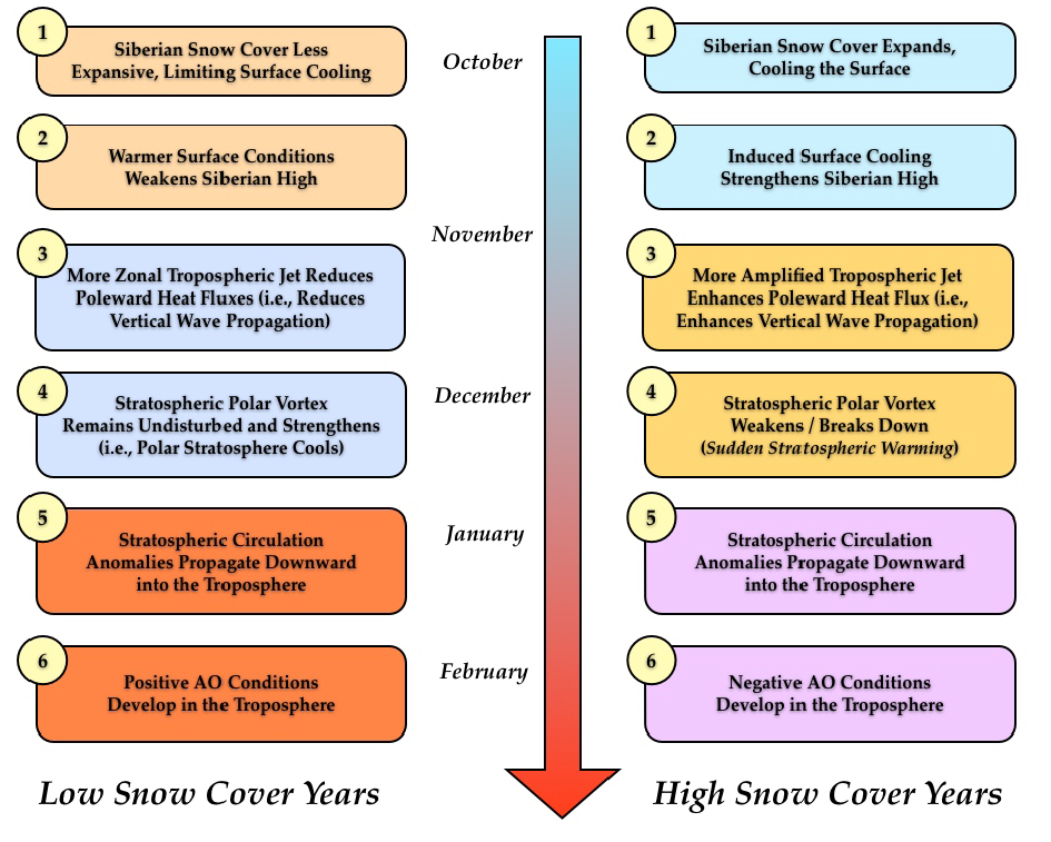
The diagram represents how Dr. Judah Cohen pictures the Northern Hemisphere wintertime climate system.  He leads research regarding Arctic and NH weather patterns for AER.

cohen-schematic2

Dr. Cohen explains the mechanism in this diagram.

Conceptual model for how fall snow cover modifies winter circulation in both the stratosphere and the troposphere–The case for low snow cover on left; the case for extensive snow cover on right.

1. Snow cover increases rapidly in the fall across Siberia, when snow cover is above normal diabatic cooling helps to;
2. Strengthen the Siberian high and leads to below normal temperatures.
3. Snow forced diabatic cooling in proximity to high topography of Asia increases upward flux of energy in the troposphere, which is absorbed in the stratosphere.
4. Strong convergence of WAF (Wave Activity Flux) indicates higher geopotential heights.
5. A weakened polar vortex and warmer down from the stratosphere into the troposphere all the way to the surface.
6. Dynamic pathway culminates with strong negative phase of the Arctic Oscillation at the surface.

From Eurasian Snow Cover Variability and Links with Stratosphere-Troposphere
Coupling and Their Potential Use in Seasonal to Decadal Climate Predictions by Judah Cohen.

Observations of the Snow Climate Factor

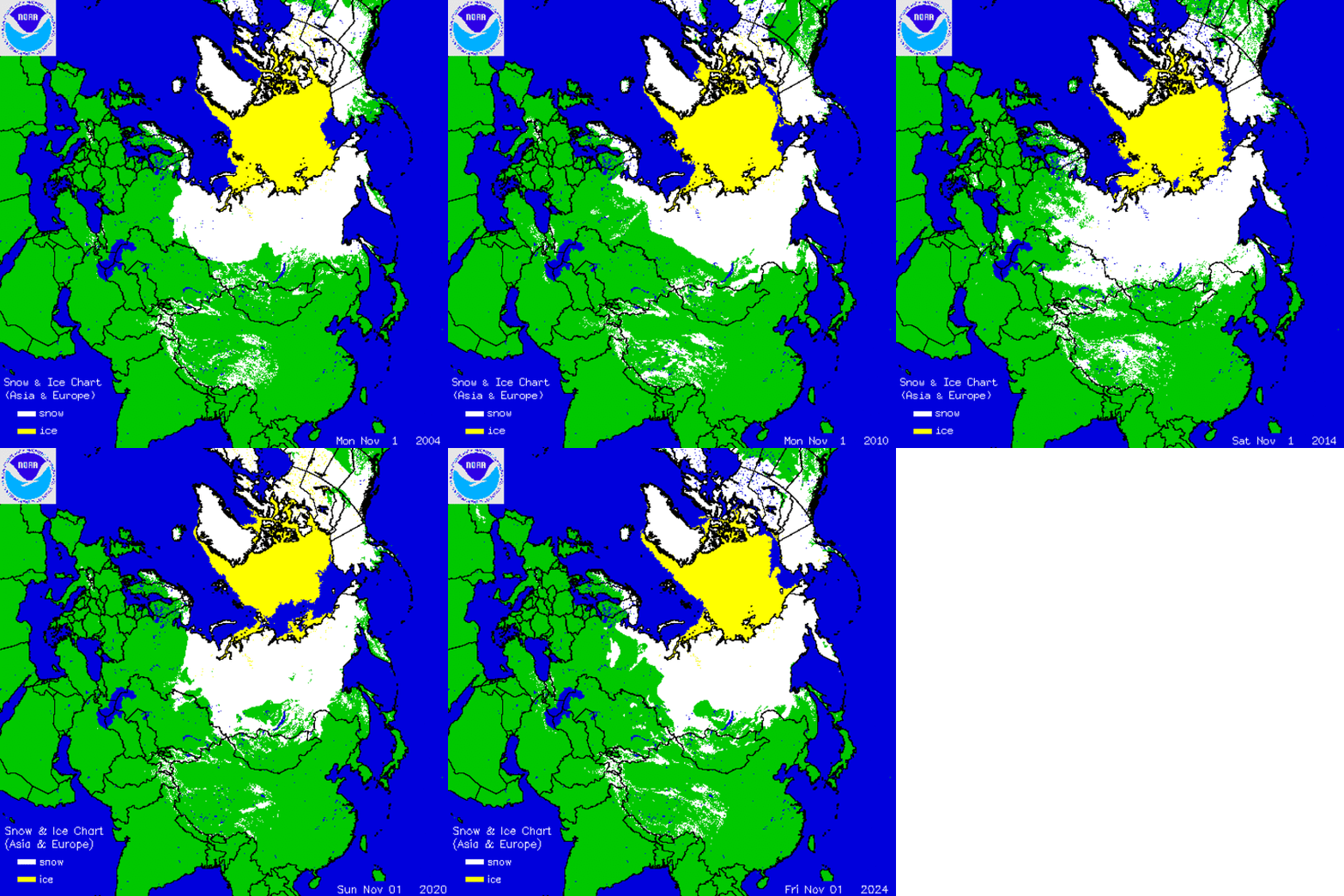
The animation at the top shows from remote sensing that Eurasian snow cover fluctuates significantly from year to year, taking the end of October as a key indicator.

For more than five decades the IMS snow cover images have been digitized to produce a numerical database for NH snow cover, including area extents for Eurasia. The NOAA climate data record of Northern Hemisphere snow cover extent, Version 1, is archived and distributed by NCDC’s satellite Climate Data Record Program. The CDR is forward processed operationally every month, along with figures and tables made available at Rutgers University Global Snow Lab.

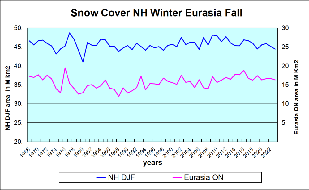
This first graph shows the snow extents of interest in Dr. Cohen’s paradigm. The Autumn snow area in Siberia is represented by the annual Eurasian averages of the months of October and November (ON). The following NH Winter is shown as the average snow area for December, January and February (DJF). Thus the year designates the December of that year plus the first two months of the next year.

Notes: NH snow cover minimum was 1981, trending upward since.  Siberian autumn snow cover was lowest in 1989, increasing since then.  Autumn Eurasian snow cover is about 1/3 of Winter NH snow area. Note also that fluctuations are sizable and correlated.

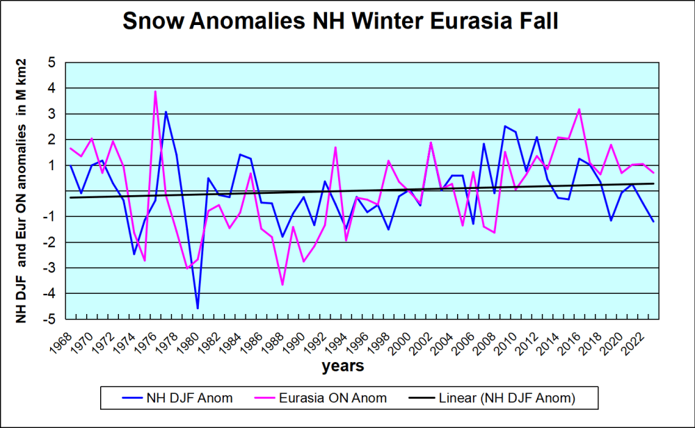
The second graph presents annual anomalies for the two series, each calculated as the deviation from the mean of its entire time series. Strikingly, the Eurasian Autumn flux is on the same scale as total NH flux, and closely aligned. While NH snow cover declined a few years prior to 2016, Eurasian snow has trended upward afterward.  If Dr. Cohen is correct, NH snowfall will follow. The linear trend is slightly positive, suggesting that fears of children never seeing snowfall have been exaggerated. The Eurasian trend line (not shown) is almost the same.

Illustration by Eleanor Lutz shows Earth’s seasonal climate changes. If played in full screen, the four corners present views from top, bottom and sides. It is a visual representation of scientific datasets measuring ice and snow extents.


Straight Talk on Climate Science and Net Zero

Michael Simpson of Sheffield University did the literature review and tells it like it is in his recent paper The Scientific Case Against Net Zero: Falsifying the Greenhouse Gas Hypothesis published at Journal of Sustainable Development (2024).  Excerpts in italics with my bolds and added images.

Abstract

The UK Net Zero by 2050 Policy was undemocratically adopted by the UK government in 2019. Yet the science of so-called ‘greenhouse gases’ is well known and there is no reason to reduce emissions of carbon dioxide (CO2), methane (CH4), or nitrous oxide (N2O) because absorption of radiation is logarithmic. Adding to or removing these naturally occurring gases from the atmosphere will make little difference to the temperature or the climate. Water vapor (H2O) is claimed to be a much stronger ‘greenhouse gas’ than CO2, CH4 or N2O but cannot be regulated because it occurs naturally in vast quantities.

This work explores the established science and recent developments in scientific knowledge around Net Zero with a view to making a rational recommendation for policy makers. There is little scientific evidence to support the case for Net Zero and that greenhouse gases are unlikely to contribute to a ‘climate emergency’ at current or any likely future higher concentrations. There is a case against the adoption of Net Zero given the enormous costs associated with implementing the policy, and the fact it is unlikely to achieve reductions in average near surface global air temperature, regardless of whether Net Zero is fully implemented and adopted worldwide. Therefore, Net Zero does not pass the cost-benefit test. The recommended policy is to abandon Net Zero and do nothing about so-called ‘greenhouse gases’. [Topics are shown below with excerpted contents.]

1. Introduction

The argument for Net Zero is that the concentration of CO2 in air is increasing, some small portion of which may be due to human activities and that Net Zero will address this supposed ‘problem’. The underpinning consensus hypothesis is that the human emission of so-called ‘greenhouse gases’ will increase concentrations of these gases in the atmosphere and thereby increase the global near surface atmospheric temperature by absorbance of infrared radiation leading to catastrophic changes in the weather. This leads to the idea that global temperatures should be limited to 2°C and preferably 1.5°C to avoid catastrophic climate change (Paris Climate Agreement, 2015).

A further hypothesis is that there are tipping points in the climate system which will result in positive feedback and a runaway heating of the planet’s atmosphere may occur (Schellnhuber & Turner, 2009; Washington et al., 2009; Levermann et al., 2009; Notz & Schellnhuber, 2009; Lenton et al., 2008; Dakos et al., 2009; Archer et al., 2009). Some of these tipping point assumptions are built into faulty climate models, the outputs of which are interpreted as facts or evidence by activists and politicians. However, output from computer models is not data, evidence or fact and is controversial (Jaworowski, 2007; Bastardi, 2018; Innis, 2008: p.30; Smith, 2021; Nieboer, 2021; Craig, 2021). Only empirical scientifically established facts should be considered so that cause and effect are clear.

From the point of view of physics, the atmosphere is an almost perfect example of a stable system (Coe, et al., 2021). The climate operates with negative feedback (Le Chatelier’s Principle) as do most natural systems with many degrees of freedom (Kärner, 2007; Lindzen et al., 2001 & 2022). The ocean acts as a heat sink, effectively controlling the air temperature. Recent global average surface temperatures remain relatively stable (Easterbrook, 2016; Moran, 2015; Morano, 2021; Marohasy, 2017; Ridley, 2010) or warming very slightly from other causes (Sangster, 2018) and the increase in temperature from 1880 through 2000 is statistically indistinguishable from 0°K (Frank, 2010; Statistics Norway, 2023) and is less than predicted by climate models (Fyfe, 2013). This shows the difference between the consensus view and established facts.

The results imply that the effect of man-made CO2 emissions does not appear to be sufficiently strong to cause systematic changes in the pattern of the temperature fluctuations. In other words, our analysis indicates that with the current level of knowledge, it seems impossible to determine how much of the temperature increase is due to emissions of CO2. Dagsvik et al. 2024

The IPCC has produced six major assessment reports (AR1 to 6) and several special reports which report on a great deal of good science (Noting that the IPCC does not do any science itself but merely compiles literature reviews). The Summaries for Policy Makers (SPM) are followed by most politicians. Yet the SPM do not agree in large part with the scientific assessment by the IPCC reports and appear to exaggerate the role of CO2 and other ‘greenhouse gases’ in climate change. It appears that the SPM is written by governments and activists before  the scientific assessment is reached which is a questionable practice (Ball 2011, 2014 and 2016; Smith 2021).

Other organizations have produced reports of a similar nature and using a similar literature (e.g. Science and Public Policy Institute; The Heartland Institute; The Centre for the Study of CO2; CO2 Science; Global Warming Policy Foundation; Net Zero Watch; The Fraser Institute; CO2 Coalition) and arrived at completely different conclusions to the IPCC and the SPM (Idso et al., 2013a; Idso et al., 2013b; Idso et al., 2014; Idso et al., 2015a, 2015b; Happer, et al., 2022). There are also some web pages (e.g. Popular Technology) which list over a thousand mainstream journal papers casting doubt on the role of CO2 and other greenhouse gases as a source of climate change. For example, a recent report by the CO2 Coalition (2023) states clearly Net Zero regulations and actions are scientifically invalid because they:

  • “Fabricate data or omit data that contradict their conclusions.
  • Rely on computer models that do not work.
  • Rely on findings of the Intergovernmental Panel on Climate Change (IPCC) that are government opinions, not science.
  • Omit the extraordinary social benefits of CO2 and fossil fuels.
  • Omit the disastrous consequences of reducing fossil fuels and CO2 emissions to Net Zero.
  • Reject the science that demonstrates there is no risk of catastrophic global warming caused by fossil fuels and CO2.

Net Zero, then, violates the tenets of the scientific method that for more than 300 years has underpinned the advancement of western civilization.” (CO2 Coalition, 2023; p. 1)

With such a strong scientific conviction the entire Net Zero agenda needs investigating. This paper reviews some of the important science which supports and undermines the Net Zero agenda.

2. Material Studied

A literature review was carried out on various topics related to greenhouse gases, climate change and the relevant scientific literature from the last 20 years in the areas of physics, chemistry, biology, paleoclimatology, geology etc. The method used was an evidence-based approach where several issues were critically evaluated based on fundamental knowledge of the science, emerging areas of scientific investigation and developments in scientific methods. The evidence-based approach is widely used (Green & Britten, 1998; Odom et al., 2005; Easterbrook, 2016; Pielke, 2014; IPCC, 2007a; IPCC 2007b; Field, 2012; IPCC 2014; McMillan & Shumacher, 2013).

Evidence-based research uses data to establish cause and effect relationships which are known to work and allows interventions which are therefore expected to be effective.

3. Greenhouse Gas Theory

The historical development of the greenhouse effect, early discussions and controversies are presented by Mudge (2012) and Strangeways (2011). The explanation of the greenhouse effect or greenhouse gas theory of climate change is given in the IPCC Fourth Assessment Report Working Group 1, The Physical Science Basis (IPCC, 2007, p. 946):

“Greenhouse gases effectively absorb thermal infrared radiation emitted by the Earth’s surface, by the atmosphere itself due to some gases, and by clouds. Atmospheric radiation is emitted to all sides, including downward to the Earth’s surface. Thus, greenhouse gases trap heat within the surface-troposphere system. This is called the greenhouse effect.”

This is plausible but does not necessarily lead to global warming as radiation will be emitted at longer wavelengths in other areas of the electromagnetic spectrum where greenhouse gases do not absorb radiation potentially leading to an energy balance without increase in temperature. To further complicate matters the definition continues with the explanation:

“Thermal infrared radiation in the troposphere is strongly coupled to the temperature of the atmosphere at the altitude at which it is emitted. In the troposphere, the temperature generally decreases with height. Effectively, infrared radiation emitted to space originates from an altitude with a temperature of, on average, -19°C in balance with the net incoming solar radiation, whereas the Earth’s surface is kept at a much higher temperature of, on average, +14°C. An increase in the concentration of greenhouse gases leads to an increased infrared opacity of the atmosphere, and therefore to an effective radiation into space from a higher altitude at a lower temperature. This causes a radiative forcing that leads to an enhancement of the greenhouse effect, the so-called enhanced greenhouse effect.”

This sort of statement is not comprehensible to the average person, makes no sense scientifically and is immediately falsified by recent research (Seim and Olsen, 2020; Coe etal., 2021; Lange et al., 2022, Wijngaarden & Happer, 2019, 2020, 2021(a), 2021(b), 2022, Sheahen, 2021; Gerlich & Tscheuschner, 2009; Zhong & Haigh, 2013). It also contradicts the work of Gray (2015 and 2019) and others and has been heavily criticized (Plimer, 2009; Plimer, 2017; Carter, 2010).

3.1 The Falsifications of the Greenhouse Effect

There are numerous falsifications of the greenhouse gas theory (sometimes called ‘trace gas heating theory’, see Siddons in Ball, 2011, p.19), of global warming and/or climate change (Ball, 2011; Ball, 2014; Ball, 2016; Gerlich & Tscheuschner, 2009; Hertzberg et al, 2017; Allmendinger, 2017; Blaauw, 2017; Nikolov and Zeller, 2017).

Fundamental empirically derived physical laws place limits on any changes in the atmospheric temperature unless there is some strong external force (e.g. increased or decreased solar radiation). For example, the Ideal Gas Law, the Beer-Lambert Law, heat capacities, heat conduction etc., (Atkins & de Paula, 2014; Barrow, 1973; Daniels & Alberty, 1966) all place physical limits on the amount of warming or cooling one might see in the climate system given any changes to heat from the sun or other sources.

3.1.1 The Ideal Gas Law

PV = nRT (1)

The average near-surface temperature for planetary bodies with an atmosphere calculated from the Ideal Gas Law is in excellent agreement with measured values suggesting that the greenhouse effect is very small or non-existent (Table 1). It is thought that the residual temperature difference of 33K between the Stephan-Boltzmann black body effective temperature (255K) on Earth and the measured near-surface temperature (288K) is caused by adiabatic auto-compression (Allmendinger, 2017; Robert, 2018; Holmes 2017, 2018 and 2019). An alternative view of this is given by Lindzen (2022). There is no need for the ‘greenhouse effect’ to explain the near surface atmospheric temperature of planetary bodies with atmospheric pressures above 10kPa (Holmes, 2017). The ideal gas law is robust and works for all gases.

3.1.2 Measurement of Infrared Absorption of the Earth’s Atmosphere

It is now possible to calculate the effect of ‘greenhouse gases’ on the surface atmospheric temperature by (a) using laboratory experimental methods; (b) using the Hitran database (https://hitran.org/); (c) using satellite observations of outgoing radiation compared to Stephan-Boltzmann effective black body radiation and calculated values of temperature.

The near surface temperature and change in surface temperature can be calculated. The result is that climate sensitivity to doubling concentration of CO2 is (0.5°C) including 0.06°C from CH4 and 0.08°C from N2O which is so small as to be undetectable. Most of the temperature change has already occurred and increasing CO2, CH4, N2O concentrations will not lead to significant changes in air temperatures because absorption is logarithmic (Beer-Lambert Law of attenuation) – a law of diminishing returns.

Figure 1. Delta T vs CO2 concentration

The important point here is that the Ideal Gas Law, the logarithmic absorption of radiation and the theoretical calculations by Wijngaarden & Happer (2020 and 2021), Coe et al., (2021) based on the Beer-Lambert Law and the Stephan-Boltzmann Law show that there is an upper limit to the temperature change which can occur by adding ‘greenhouse gases’ to the atmosphere if the main source of incoming radiation (the Sun) does not change over time. The upper limit is ~0.81°C.

3.1.3 Other Falsifications

Many climatologists ignore the well-established ideas of the Ideal Gas Law, Kinetic Theory of Gases and Collision Theory which explain the interaction of gases in the atmosphere (Atkins & de Paula, 2014; Salby, 2012; Tec science). For example, it is difficult for CO2 to retain heat energy (by vibration, rotation, and translation) as there are 1034 collisions between air molecules per second per cubic meter of gas at a pressure of 1 atmosphere (~101.3kPa) and on each collision, energy is exchanged leading to a Maxwell-Boltzmann distribution (similar to a normal distribution) of molecular energies across all molecules in air (Tec science). The Maxwell-Boltzmann distribution has been experimentally determined (Atkins & de Paula, 2014). Thus, the major components of air (nitrogen and oxygen) retain most of the energy, cause evaporation of water vapor by heat transfer (mainly by conduction and convection) and emit radiation at longer wavelengths. The small concentration of CO2 in air (circa 420ppmv) cannot account for large changes in the climate system which have occurred in the past (Wrightstone, 2017 and 2023; Ball, 2014). Plimer (2009 and 2017) presents a great deal of geological scientific evidence which covers paleoclimatology concluding that:

“There is no such thing as the greenhouse effect. The atmosphere behaves neither as a greenhouse nor as an insulating blanket preventing heat escaping from the Earth. Competing forces of evaporation, convection, precipitation, and radiation create an energy balance in the atmosphere.” (Plimer 2009: p.364).

Ball (2014) summarizes a great deal of the geological science:

“The most fundamental assumption in the theory that human CO2 is causing global warming and climate change is that an increase in CO2 will cause an increase in temperature. The problem is that every record of any duration for any period in the history of the Earth exactly the opposite relationship occurs temperature increase precedes CO2 increase. Despite that a massive deception has developed and continues.” Ball (2014: p. 1).

This statement agrees with many other scientists working in geology, earth sciences, physics and physical chemistry as can be seen in cited references in books (Easterbrook, 2016; Wrightstone 2017 and 2023; Plimer, 2009; Plimer 2017; Ball, 2014; Ball,2011; Ball, 2016; Carter, 2010; Koutsoyiannis et al, 2023 & 2024; Hodzic, and Kennedy, 2019). Easterbrook (2016) uses the evidence-based approach to climate science and concludes that:

“Because of the absence of any physical evidence that CO2 causes global warming, the main argument for CO2 as the cause of warming rests largely on computer modelling.”  Easterbrook (2016: p.5).

The results of the models are projected far into the future (circa 80 to 100years) where uncertainties are large, but projections can be used to demonstrate unrealistic but scary scenarios (Idso et al., 2015b). The literature that is used for the IPCC reports appears to be ‘cherry picked’ to agree with their paradigms that increasing CO2 concentrations leads to warming. They ignore the vast literature in climatology, atmospheric physics, solar physics, physics, physical chemistry, geology, biology and palaeoclimatology much of which contradicts the IPCC’s assessment in the summary for policymakers (SPM).

The objective of the IPCC was to find the human causes of climate change – not to look at all the causes of climate change which would be the sensible thing to do if the science were to be used to inform policy decisions. However, there is no experimental evidence for a significant anthropogenic component to climate change (Kaupinnen and Malmi, 2019) which leaves genuine scientists and citizens concerned about the role of the IPCC.

3.1.4 Anthropogenic CO2 and the Residence time of Carbon Dioxide in Air

There is a suggestion (IPCC) that the residence time of CO2 in the atmosphere is different for anthropogenic CO2 and naturally occurring CO2. This breaks a fundamental scientific principle, the Principle of Equivalence. That is: if there is equivalence between two things, they have the same use, function, size, or value (Collins English Dictionary, online). Thus, CO2 is CO2 no matter where it comes from, and each molecule will behave physically and react chemically in the same way.

The figures above illustrate how exaggerated claims are made for CO2 based on the false assumption that CO2 resides in the atmosphere for long periods and can affect the climate. These results are enough to falsify the ideas of anthropogenic global warming caused by CO2 and shows how little human activity contributes to CO2 emissions and concentrations in air. The argument is clear, that if the fictitious greenhouse effect were real for CO2 the human contribution would have no measurable effect upon the climate in terms of global average surface temperature.

The residence time of CO2 in the atmosphere is between 3.0 and 4.1 years using the IPCC’s own data and not the supposed 100 years or 1000 years for anthropogenic CO2 suggested by the IPCC summaries for policy makers (Harde, 2017) which contravenes the Equivalence Principle (Berry, 2019).

“These results indicate that almost all of the observed change of CO2 during the industrial era followed, not from anthropogenic emission, but from changes of natural emission. The results are consistent with the observed lag of CO2 changes behind temperature changes (Humlum et al., 2013; Salby, 2013), a signature of cause and effect.” (Harde, 2017a: 25).

It is well-known that the residence time of CO2 in the atmosphere is approximately 5 years (Boehmer-Christiansen, 2007: 1124; 1137; Kikuchi, 2010). Skrable et al., (2022), show that accumulated human CO2 is 11% of CO2 in air or ~46.84ppmv based on modelling studies. Berry (2020, 2021) uses the Principle of  Equivalence (which the IPCC violates by assuming different timescales for the uptake of natural and human CO2) and agrees with Harde (2017a) that human CO2 adds about 18ppmv to the concentration in air. These are physically extremely small concentrations of CO2 which suggest most CO2 arises from natural sources. It can be concluded that the IPCC models are wrong and human CO2 will have little effect on the temperature.

4. Conclusions

Like many other researchers it was assumed there was robust science behind the greenhouse gas theory and that Net Zero was essential to achieve, but after investigation it now appears that the greenhouse gas theory is questionable and has been successfully challenged for at least 100 years (Gerlich and Tscheuschner, 2009). Much better explanations for planetary near surface atmospheric temperatures are available based on robust, empirically derived scientific laws such as the Ideal Gas law.

Better assessments of the potential increase in temperature with doubling CO2 concentrations are available and the calculated increase is small ~0.5°C (Coe et al., 2021; van Wijngaarden & Happer, 2019, 2020 and 2021; Sheahen, 2021; Schildknecht, 2020) and will remain very small with increased CO2 concentration because the infrared CO2 absorption bands are almost saturated and absorption follows the logarithmic Beer-Lambert law (Figure 1). Much of the work using the Hitran database has been tested against satellite measurements of the outgoing radiation from the Earth’s atmosphere and the calculations are in almost perfect agreement (Sheahen, 2021).

This suggests that the physicists are correct in their assessment of the likely very small increase in atmospheric temperature and therefore there is a strong case against Net Zero as it will have no discernible effect on temperature and the cost of Net Zero is huge. Therefore, the Net Zero project does not pass the cost-benefit test (Montford, 2024b; NESO, 2024). That is the costs are disproportionately high for little or no benefit. Thus, the correct response to a non-problem is to do nothing. The monies being wasted on Net Zero should be spent for the benefit of citizens (e.g. education, health care, public health, water infrastructure, waste processing, economic prosperity etc.). There are many other pressing public health problems from burning fossil fuels which should be addressed (e.g. air pollution especially particulates and carbon monoxide).

Better calculations of the human contribution to atmospheric CO2 concentrations are available and it is small ~18ppmv (Skrable et al., 2022; Berry, 2020; Harde 2017a & 2017b; Harde, 2019; Harde 2014). The phase relation between temperature and CO2 concentration changes are now clearly understood; temperature increases are followed by increases in CO2 likely from outgassing from the ocean and increased biological activity (Davis , 2017; Hodzic and Kennedy, 2019; Humlum, 2013; Salby, 2012; Koutsoyiannis et al, 2023 & 2024).

“In conclusion on the basis of observational data, the climate crisis that, according to many sources, we are experiencing today, is not evident yet.” Alimonti etal. 2022: 111.

Many researchers are addressing the ‘CO2 and climate change problem’ by suggesting decarbonization and other approaches such as Net Zero. CO2 is more than likely not the temperature control and has a very minor to negligible role in global warming (The Bruges Group, 2021; De Lange and Berkhout, 2024; Manheimer, 2022; Statistics Norway 2023; Lindzen and Happer, 2024; Lindzen, et al., 2024).

The scientific literature was examined and found to provide several alternative views concerning CO2 and the need for Net Zero. The objectives of this paper have been achieved and the conclusions can be briefly summarized:

  1. CO2 is a harmless highly beneficial rare trace gas essential for all life on Earth due to photosynthesis which produces simple sugars and carbohydrates in plants and a bi-product Oxygen (O2). CO2is therefore the basis of the entire food supply chain (see Biology or Botany textbooks or House, 2013). CO2 is close to an all-time low geologically (Wrightstone, 2017 and 2023) and controls on CO2 emissions and concentrations in air should be considered as very dangerous and expensive policy indeed. Net Zero is not necessary and should be abandoned.
  2. The greenhouse gas theory has been falsified (i.e. proven wrong) from several disciplines including paleoclimatology, geology, physics, and physical chemistry. CO2 cannot affect the climate in such small concentrations (~420ppmv or ~0.04%) and basing government policy on output from faulty climate models will prove to be very expensive and achieve nothing for the environment, public health, or the climate.

“There is no atmospheric greenhouse effect, in particular CO2 greenhouse effect, in theoretical physics and engineering thermodynamics. Thus, it is illegitimate to deduce predictions which provide a consulting solution for economics and intergovernmental policy.” (Gerlich & Tscheuschner, 2009: 354).

  1. The oceans contain approximately 50 times as much CO2 as is currently present in the air (Easterbrook, 2016; Wrightstone, 2017 and 2023) and as such Henry’s Law will work to maintain the dynamic equilibrium concentration in air over the longer term as the ocean will absorb and outgas CO2(Atkins & de Paula, 2014). Net Zero will, therefore, achieve nothing for the concentration of CO2 in the atmosphere. If the volcanic sources of CO2 are as Kamis (2021), the IPCC and others suggest many times the human contribution, then Net Zero will have no measurable effect on atmospheric CO2 concentrations. Net Zero should, therefore, be abandoned.
  2. The contribution to greenhouse gases, especially CO2, attributable to humans is extremely small, almost negligible (~4.3% or ~18ppmv total accumulation) and half is absorbed by the ocean and biomass. Other naturally occurring so-called greenhouse gases are present in very small/negligible quantities (e.g. CH4, N2O). The systematic attempts to eliminate these trace gases from the atmosphere by reducing industrial output, reducing farming, eliminating fossil fuel use, and changing the way human civilization lives is totally unnecessary – again the ‘do-nothing strategy’ is strongly recommended.
  3. The sciences have been largely ignored by politicians and activists. There have been numerous failings of governments to take notice of scientific findings and they have succumbed to unnecessary pressure from activist groups (including the United Nations and the IPCC). Net Zero is just one example where costly efforts by governments will achieve nothing and not address the real problems of air pollution, public health, or economic well-being of citizens.

“There is not a single fact, figure or observation that leads us to conclude that the world’s climate is in any way disturbed.” (Société de Calcul Mathématique SA, 2015:3).

  1. Circular reasoning is used by the climate modelers. That is, the fictitious greenhouse effect is built into the models such that when the parameter of CO2concentration is increased then the temperature output of the models increases, producing models which run relatively hot compared to natural variability. This reduces the so-called greenhouse effect to little more than a ‘fudge factor’ or ‘parameter’ within models which essentially gives you the answer that you set out to prove. This circular reasoning is hardly scientific enquiry and with data ‘homogenization’ and infilling of missing data begins to look rather peculiar. Climatologists need to recognize these issues, address the real reasons for climate change and offer genuine solutions to any real problems.
  2. The claim of consensus is completely unscientific in its approach (Idso et al, 2015a). Noting that 31,000 US scientists and engineers signed the petition protest (Robinson et al., 2007), recently 90 Italian scientists wrote an open letter to the Italian government (Crescenti et al., 2019), and 500 climatologists and scientists signed an open letter to the UN Secretary General (Berkhout, 2019). All explaining that CO2 is not the cause of climate change. There are thousands of academic papers and books questioning anthropogenic climate change with good data.

Many other concerned individuals have looked at the evidence for anthropogenic climate change based on CO2 and found it wanting (e.g. Davison, 2018; Rofe, 2018).

“If in fact ‘the science is settled’, it seems to be much more settled in the fact that there is no particular correlation between CO2 level and the earth’s temperature.” (Manheimer, 2022).

and

“If you assume the Intergovernmental Panel on Climate Change are right about everything and use only their numbers in the calculation, you will arrive at the conclusion that we should do nothing about climate change!” (Field, 2013).

The academic literature in science offers numerous and far better explanations for climate change than the fictitious greenhouse effect. Researchers should recognize this fact and start to look at dealing with the real causes of climate change. Net Zero is an enormously expensive solution to a non-problem and has no obvious redeeming features. The Net Zero policy is not financially sustainable and should be abandoned.



Movement for Sensible Climate Policy

Many of us are blogging to draw attention to knowledge and information dismissed or suppressed by legacy and social media as “misinformation”, simply because the thoughts and ideas are rational and reasonable rather than alarmist. Tom Harris reminded me in his recent comment that we have many many colleagues speaking out in the public square sharing our concerns.  So let this post introduce a valuable resource in this fight for reasonable climate understandings and policies, namely CANADIANS FOR  SENSIBLE CLIMATE POLICY Join the Movement for Responsible and Sensible Climate Policy.

The home page summarizes why this mission is important and what is at stake and the path forward.

Climate Activism is BIG business

The Green Budget Coalition in 2024 is made up of 21 of the leading Canadian environmental activist organizations publicly lobbying for $287 billion in government spending on their causes.
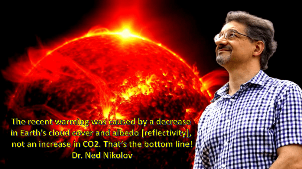
That is 62% of the total federal tax revenue.

According to public data, in Canada alone these organizations control billions in funds, raise and spend millions on PR campaigns and employ hundreds of staff to achieve these objectives. Globally, the climate activism industry controls trillions of dollars and has armies of advocates. This politicisation of public policy impacts every Canadian.
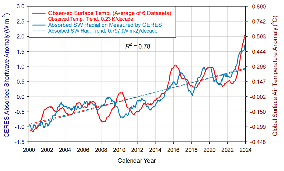
Even when done with the best intentions, power without oversight isn’t peace, order or good government. To advocate for the best policy, we encourage a range of views, even the controversial ones. We dare to question, to be wrong and to explore all sides of complex issues.

What matters is adopting sober, reasonable and sensible policy in the interests of all Canadians.

Our Concerns

Strange Math

Carbon dioxide gets a lot of attention compared to the many other environmental concerns. Every bad weather event gets assigned to it. The main player in the greenhouse effect remains water and clouds. A changing climate may be unpredictable but that does not mean abnormal.

With prosperity comes costs which must be balanced against the benefits. Strange does not mean unexplainable. Proclamations of doom and crisis are always suspicious.

Odd incentives

Big Oil, corporate interests, corrupt politicians, conspiracy theorists, corporate PR firms and paid skeptics. These are all boogeymen for why, despite general popularity and political backing, there remains a dire crisis with minimal progress.

What if the crisis is exactly because the incentives are designed to perpetuate a cycle? What if the problem isn’t bad intentions or ethics but a social mission over funded to irreverence which needs to be called out as ineffective?

Motivated Reasoning

Motivated reasoning is choosing only the good parts of a story while ignoring the rest because it is what we want to believe. It is quite common in everyday life. When it comes to climate change, calm, pragmatic discussions are rare with many complex and passionate explanations and perspectives.

Those complex explanations may well be accurate, but any analysis of climate change must acknowledge the issue has emotional and personal implications for many Canadians.

Outsourced Problems

When speaking unpopular opinions, one’s intelligence, integrity and ethics will almost always come under fire. When speaking popular opinions rarely is there such scrutiny. It’s human to deeply care for our environment. Why don’t we see the mass implementation of responsible governance, moderation & sustainability? Why so much green washing? Why are 9/10 solutions just shifting our problems into other people’s lands.

Transporting environmental destruction from Canada to Qatar, China or Nigeria is not ethical or effective. If being sustainable was easy or obvious someone would have done it long ago.

Little Accountability

Spending must be within context. Canada is estimated to produce about 2% of the worlds total CO2 emissions with our higher emissions per capita being within expectations for an oil producing nation. Alberta accounts for much of this higher status. The Federal government revenue was $447 billion. A provincial government like Ontario was $179 billion.

A hundred billion or trillion dollar public effort to reduce a rounding error in emissions isn’t just another project, it’s a significant financial commitment with long lasting implications.

Boomers

Your generation has enjoyed a splendid life because of the sacrifices made by your parents during and after WW2. Post war, jobs were easy to find, economies expanded throughout the developed world and Boomers “Never-had-it-so-good.” In retirement your lifestyle was far better than any previous generation enjoyed.

Now, you have a choice, you can either watch economic hardship unfold while passing on huge debts to the next generations or speak up and blow the whistle on the biggest waste of capital the world has ever seen.

Non-Boomers

You are inheritors of a huge debt by the leadership of today. Do you want to spend your life in bad economic times? Do you want your children to live through the same hardships as you stand to inherit? How much time have you invested in thinking about what the Net Zero at 2050 policies cost? Can humans in fact control climate? Is the financial sector pushing that agenda biased? Are the alternative energy jobs long-term or busy-work?

Decide for yourself. Make your thoughts known.

Course Correction

Cost-Benefit Accounting

Alberta and Saskatchewan’s embrace of lower-regulation, pro-petroleum and chemical development is a source of concern to many Canadians. Yet, this comes with benefits to those same groups including massive subsidies to public spending, foreign investment, increased buying power and lowered cost of living in all provinces.

A sensible climate policy transcends politicisation, it works for those who are pro-petroleum or anti-petroleum, left or right wing, those who see increased carbon as beneficial or those seeking net-zero. Sober energy policy improves lives by balancing concerns and offering pragmatic decisions which achieve universal objectives.

Open Discussion

The journalists spread the word and the activists too, the science becomes “settled” and 97% of climate scientists agree. Your life could get a little easier, just don’t listen to skeptics, realists, opponents, the scientists not surveyed, friends, brothers, sisters, cousins, or uncles. An agency will sort the details and inform you of the correct and proper truth.

Never, a sensible climate policy comes from open inquiry, where facts and data are the observations in agreement and the debate is about the meaning and impacts of that data. Experts will breakdown confusion, answer questions and offer clarity.

Prioritize the Everyday Canadian

Climate change policies and activism have a track record of growing budgets, increased powers, and increased access to new technologies and insights. Show us the benefits. Show us the increases in quality of life. Show the practical applications and decreased risks and dangers.

A sensible climate policy is measurable, and though perhaps driven by fear and concern, increased attention and effort means more tangible results.

Maximize Well-being

In cost-benefit analysis, choices are made between conflicting values. Energy and climate policy can be framed as altruists against economics. It can be framed as common good against special interests. It can be framed as differing scientific views.

A sensible climate policy will be driven by maximizing well-being and benefit to society.

Ensure Accountability

Climate policy is often ignored except by special interests. The tale of energy companies against the activists is contradicted by the funding patterns which see energy companies actively funding, hiring and promoting climate change activists. In the energy business “green energy” is just another opportunity.

A sensible climate policy must have checks and balances. Lobbying can benefit everyone in a marketplace of ideas but as a monopoly, everyday Canadians will never be served.