Warmists consistently do recycling, especially alarming stories coming back for encore media appearances. This week it’s the suffocating ocean meme, which taps into our caring about the seas, but conflates impacts from human maritime activities with subtle temperature changes, i.e climate change (AKA emergency, chaos, crisis etc.). Of course COP 25 is the trigger for this. I won’t list the alarming headlines since they are little different from last time, covered in a previous post reprinted below. Below are two typical recent quotes showing how an actual ocean concern is exploited for fossil fuel activism.
“A healthy ocean with abundant wildlife is capable of slowing the rate of climate breakdown substantially,” said Dr Monica Verbeek, the executive director of the group Seas at Risk. “To date, the most profound impact on the marine environment has come from fishing. Ending overfishing is a quick, deliverable action which will restore fish populations, create more resilient ocean ecosystems, decrease CO2 pollution and increase carbon capture, and deliver more profitable fisheries and thriving coastal communities.”
“Ending overfishing would strengthen the ocean, making it more capable of withstanding climate change and restoring marine ecosystems – and it can be done now,” explained Rashid Sumaila, professor and director of the fisheries economics research unit at the University of British Columbia. “The crisis in our fisheries and in our oceans and climate are not mutually exclusive problems to be addressed separately – it is imperative that we move forward with comprehensive solutions to address them.”
Previous post from last year
The climate scare machine is promoting again the fear of suffocating oceans. For example, an article this week by Chris Mooney in Washington Post, It’s Official, the Oceans are Losing Oxygen.
A large research synthesis, published in one of the world’s most influential scientific journals, has detected a decline in the amount of dissolved oxygen in oceans around the world — a long-predicted result of climate change that could have severe consequences for marine organisms if it continues.
The paper, published Wednesday in the journal Nature by oceanographer Sunke Schmidtko and two colleagues from the GEOMAR Helmholtz Centre for Ocean Research in Kiel, Germany, found a decline of more than 2 percent in ocean oxygen content worldwide between 1960 and 2010.
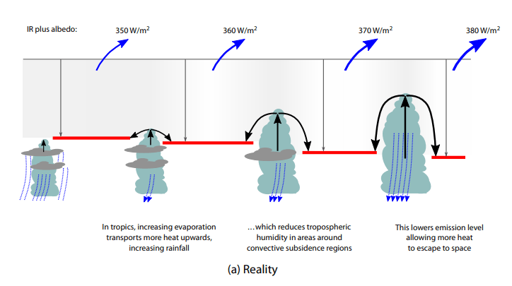
Climate change models predict the oceans will lose oxygen because of several factors. Most obvious is simply that warmer water holds less dissolved gases, including oxygen. “It’s the same reason we keep our sparkling drinks pretty cold,” Schmidtko said.
But another factor is the growing stratification of ocean waters. Oxygen enters the ocean at its surface, from the atmosphere and from the photosynthetic activity of marine microorganisms. But as that upper layer warms up, the oxygen-rich waters are less likely to mix down into cooler layers of the ocean because the warm waters are less dense and do not sink as readily.
And of course, other journalists pile on with ever more catchy headlines.
The World’s Oceans Are Losing Oxygen Due to Climate Change
How Climate Change Is Suffocating The Oceans
Overview of Oceanic Oxygen
Once again climate alarmists/activists have seized upon an actual environmental issue, but misdirect the public toward their CO2 obsession, and away from practical efforts to address a real concern. Some excerpts from scientific studies serve to put things in perspective.
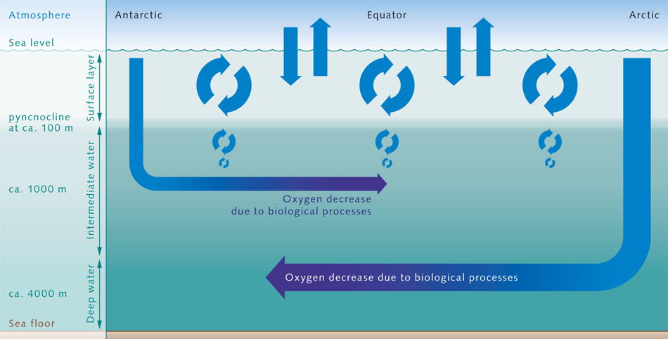
2.14 > Oxygen from the atmosphere enters the near-surface waters of the ocean. This upper layer is well mixed, and is thus in chemical equilibrium with the atmosphere and rich in O2. It ends abruptly at the pyncnocline, which acts like a barrier. The oxygenrich water in the surface zone does not mix readily with deeper water layers. Oxygen essentially only enters the deeper ocean by the motion of water currents, especially with the formation of deep and intermediate waters in the polarregions. In the inner ocean, marine organisms consume oxygen. This creates a very sensitive equilibrium.
How the Ocean Breathes
Variability in oxygen and nutrients in South Pacific Antarctic Intermediate Water by J. L. Russell and A. G. Dickson
The Southern Ocean acts as the lungs of the ocean; drawing in oxygen and exchanging carbon dioxide. A quantitative understanding of the processes regulating the ventilation of the Southern Ocean today is vital to assessments of the geochemical significance of potential circulation reorganizations in the Southern Hemisphere, both during glacial-interglacial transitions and into the future.
Traditionally, the change in the concentration of oxygen along an isopycnal due to remineralization of organic material, known as the apparent oxygen utilization (AOU), has been used by physical oceanographers as a proxy for the time elapsed since the water mass was last exposed to the atmosphere. The concept of AOU requires that newly subducted water be saturated with respect to oxygen and is calculated from the difference between the measured oxygen concentration and the saturated concentration at the sample temperature.
This study has shown that the ratio of oxygen to nutrients can vary with time. Since Antarctic Intermediate Water provides a necessary component to the Pacific equatorial biological regime, this relatively high-nutrient, high-oxygen input to the Equatorial Undercurrent in the Western Pacific plays an important role in driving high rates of primary productivity on the equator, while limiting the extent of denitrifying bacteria in the eastern portion of the basin.
Uncertain Measures of O2 Variability and Linkage to Climate Change
A conceptual model for the temporal spectrum of oceanic oxygen variability by Taka Ito and Curtis Deutsch
Changes in dissolved O2 observed across the world oceans in recent decades have been interpreted as a response of marine biogeochemistry to climate change. Little is known however about the spectrum of oceanic O2 variability. Using an idealized model, we illustrate how fluctuations in ocean circulation and biological respiration lead to low-frequency variability of thermocline oxygen.
Because the ventilation of the thermocline naturally integrates the effects of anomalous respiration and advection over decadal timescales, shortlived O2 perturbations are strongly damped, producing a red spectrum, even in a randomly varying oceanic environment. This background red spectrum of O2 suggests a new interpretation of the ubiquitous strength of decadal oxygen variability and provides a null hypothesis for the detection of climate change influence on oceanic oxygen. We find a statistically significant spectral peak at a 15–20 year timescale in the subpolar North Pacific, but the mechanisms connecting to climate variability remain uncertain.
The spectral power of oxygen variability increases from inter-annual to decadal frequencies, which can be explained using a simple conceptual model of an ocean thermocline exposed to random climate fluctuations. The theory predicts that the bias toward low-frequency variability is expected to level off as the forcing timescales become comparable to that of ocean ventilation. On time scales exceeding that of thermocline renewal, O2 variance may actually decrease due to the coupling between physical O2 supply and biological respiration [Deutsch et al., 2006], since the latter is typically limited by the physical nutrient supply.
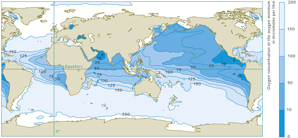
2.15 > Marine regions with oxygen deficiencies are completely natural. These zones are mainly located in the mid-latitudes on the west sides of the continents. There is very little mixing here of the warm surface waters with the cold deep waters, so not much oxygen penetrates to greater depths. In addition, high bioproductivity and the resulting large amounts of sinking biomass here lead to strong oxygen consumption at depth, especially between 100 and 1000 metres.
Climate Model Projections are Confounded by Natural Variability
Natural variability and anthropogenic trends in oceanic oxygen in a coupled carbon cycle–climate model ensemble by T. L. Frolicher et al.
Internal and externally forced variability in oceanic oxygen (O2) are investigated on different spatiotemporal scales using a six-member ensemble from the National Center for Atmospheric Research CSM1.4-carbon coupled climate model. The oceanic O2 inventory is projected to decrease significantly in global warming simulations of the 20th and 21st centuries.
The anthropogenically forced O2 decrease is partly compensated by volcanic eruptions, which cause considerable interannual to decadal variability. Volcanic perturbations in oceanic oxygen concentrations gradually penetrate the ocean’s top 500 m and persist for several years. While well identified on global scales, the detection and attribution of local O2 changes to volcanic forcing is difficult because of unforced variability.
Internal climate modes can substantially contribute to surface and subsurface O2 variability. Variability in the North Atlantic and North Pacific are associated with changes in the North Atlantic Oscillation and Pacific Decadal Oscillation indexes. Simulated decadal variability compares well with observed O2 changes in the North Atlantic, suggesting that the model captures key mechanisms of late 20th century O2 variability, but the model appears to underestimate variability in the North Pacific.
Our results suggest that large interannual to decadal variations and limited data availability make the detection of human-induced O2 changes currently challenging.
The concentration of dissolved oxygen in the thermocline and the deep ocean is a particularly sensitive indicator of change in ocean transport and biology [Joos et al., 2003]. Less than a percent of the combined atmosphere and ocean O2 inventory is found in the ocean. The O2 concentration in the ocean interior reflects the balance between O2 supply from the surface through physical transport and O2 consumption by respiration of organic material.
Our modeling study suggests that over recent decades internal natural variability tends to mask simulated century-scale trends in dissolved oxygen from anthropogenic forcing in the North Atlantic and Pacific. Observed changes in oxygen are similar or even smaller in magnitude than the spread of the ensemble simulation. The observed decreasing trend in dissolved oxygen in the Indian Ocean thermocline and the boundary region between the subtropical and subpolar gyres in the North Pacific has reversed in recent years [McDonagh et al., 2005; Mecking et al., 2008], implicitly supporting this conclusion.
The presence of large-scale propagating O2 anomalies, linked with major climate modes, complicates the detection of long-term trends in oceanic O2 associated with anthropogenic climate change. In particular, we find a statistically significant link between O2 and the dominant climate modes (NAO and PDO) in the North Atlantic and North Pacific surface and subsurface waters, which are causing more than 50% of the total internal variability of O2 in these regions.
To date, the ability to detect and interpret observed changes is still limited by lack of data. Additional biogeo-chemical data from time series and profiling floats, such as the Argo array (http://www.argo.ucsd.edu) are needed to improve the detection of ocean oxygen and carbon system changes and our understanding of climate change.
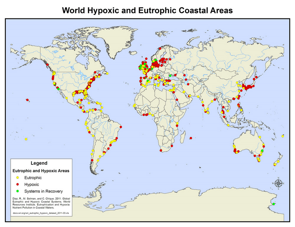
The Real Issue is Ocean Dead Zones, Both Natural and Man-made
Since 1994, he and the World Resources Institute (report here) in Washington,D.C., have identified and mapped 479 dead zones around the world. That’s more than nine times as many as scientists knew about 50 years ago.
What triggers the loss of oxygen in ocean water is the explosive growth of sea life fueled by the release of too many nutrients. As they grow, these crowds can simply use up too much of the available oxygen.
Many nutrients entering the water — such as nitrogen and phosphorus — come from meeting the daily needs of some seven billion people around the world, Diaz says. Crop fertilizers, manure, sewage and exhaust spewed by cars and power plants all end up in waterways that flow into the ocean. Each can contribute to the creation of dead zones.
Ordinarily, when bacteria steal oxygen from one patch of water, more will arrive as waves and ocean currents bring new water in. Waves also can grab oxygen from the atmosphere.
Dead zones develop when this ocean mixing stops.
Rivers running into the sea dump freshwater into the salty ocean. The sun heats up the freshwater on the sea surface. This water is lighter than cold saltier water, so it floats atop it. When there are not enough storms (including hurricanes) and strong ocean currents to churn the water, the cold water can get trapped below the fresh water for long periods.
Dead zones are seasonal events. They typically last for weeks or months. Then they’ll disappear as the weather changes and ocean mixing resumes.
Solutions are Available and do not Involve CO2 Emissions

Helping dead zones recover
The Black Sea is bordered by Europe and Asia. Dead zones used to develop here that covered an area as large as Switzerland. Fertilizers running off of vast agricultural fields and animal feedlots in the former Soviet Union were a primary cause. Then, in 1989, parts of the Soviet Union began revolting. Two years later, this massive nation broke apart into 15 separate countries.
The political instability hurt farm activity. In short order, use of nitrogen and phosphorus fertilizers by area farmers declined. Almost at once, the size of the Black Sea’s dead zone shrunk dramatically. Now if a dead zone forms there it’s small, Rabalais says. Some years there is none.
Chesapeake Bay, the United State’s largest estuary, has its own dead zone. And the area affected has expanded over the past 50 years due to pollution. But since the 1980s, farmers, landowners and government agencies have worked to reduce the nutrients flowing into the bay.
Farmers now plant cover crops, such as oats or barley, that use up fertilizer that once washed away into rivers. Growers have also established land buffers to absorb nutrient runoff and to keep animal waste out of streams. People have even started to use laundry detergents made without phosphorus.
In 2011, scientists reported that these efforts had achieved some success in shrinking the size of the bay’s late-summer dead zones.
The World Resources Institute lists 55 dead zones as improving. “The bottom line is if we take a look at what is causing a dead zone and fix it, then the dead zone goes away,” says Diaz. “It’s not something that has to be permanent.”
Summary
Alarmists/activists are again confusing the public with their simplistic solution for a complex situation. And actual remedies are available, just not the agenda preferred by climatists.

Waste Management Saves the Ocean


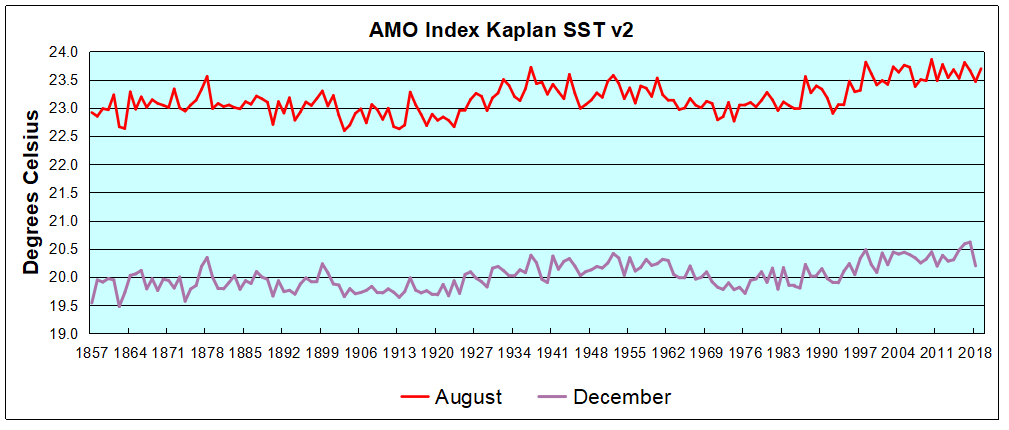
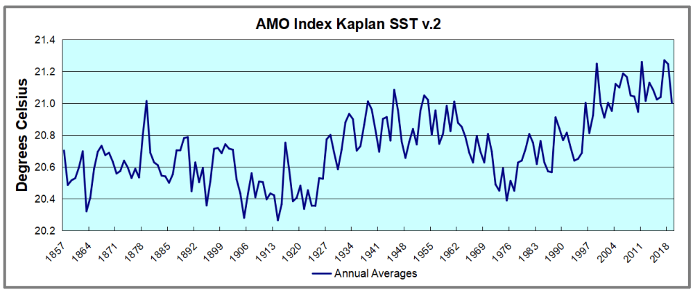
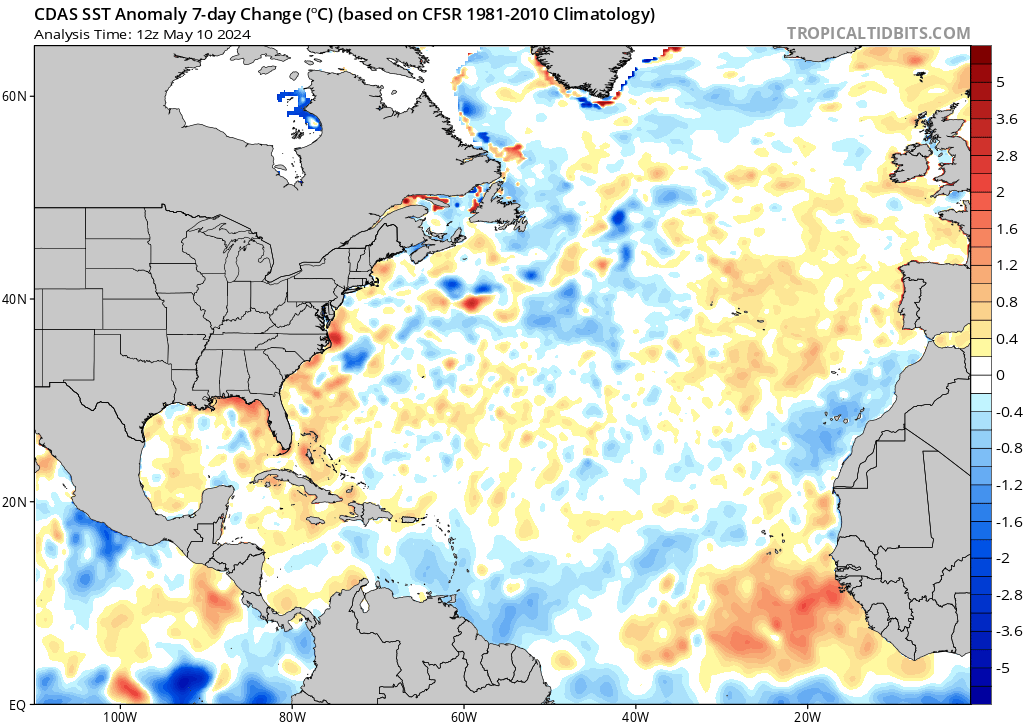
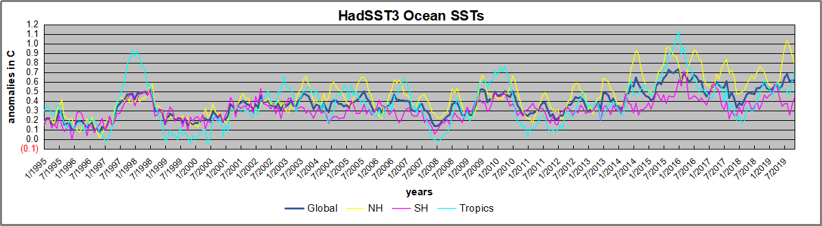
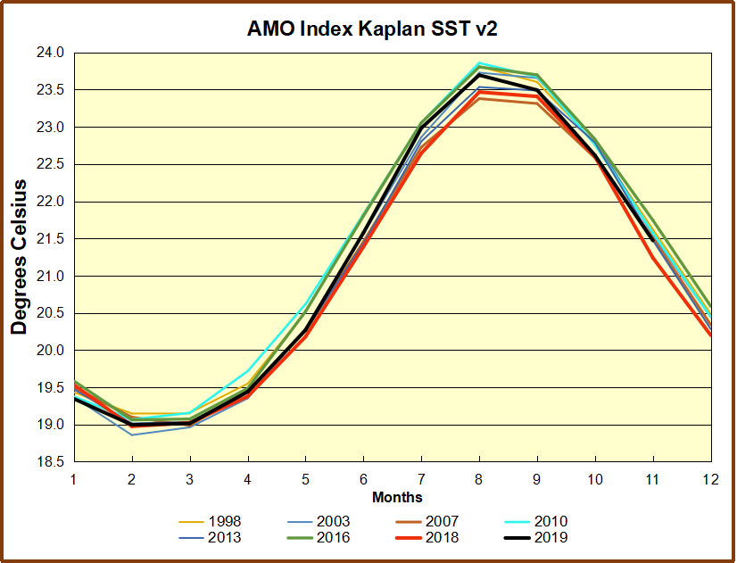
 The best context for understanding decadal temperature changes comes from the world’s sea surface temperatures (SST), for several reasons:
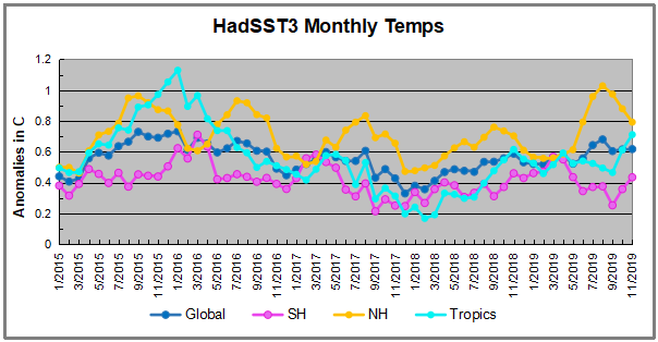


 The term “glittering generality” was impressed on me by an English teacher who red-circled several expressions in my essay with the label “GG”. When I asked what was wrong, she told me pretty much what Wikipedia says:
 “For about a year I have been constantly talking about our rapidly declining carbon budgets over and over again. But since that is still being ignored, I will just keep repeating it