With apologies to Paul Revere, this post is on the lookout for cooler weather with an eye on both the Land and the Sea. UAH has updated their tlt (temperatures in lower troposphere) dataset for November. Previously I have done posts on their reading of ocean air temps as a prelude to updated records from HADSST3. This month also has a separate graph of land air temps because the comparisons and contrasts are interesting as we contemplate possible cooling in coming months and years.
Presently sea surface temperatures (SST) are the best available indicator of heat content gained or lost from earth’s climate system. Enthalpy is the thermodynamic term for total heat content in a system, and humidity differences in air parcels affect enthalpy. Measuring water temperature directly avoids distorted impressions from air measurements. In addition, ocean covers 71% of the planet surface and thus dominates surface temperature estimates. Eventually we will likely have reliable means of recording water temperatures at depth.
Recently, Dr. Ole Humlum reported from his research that air temperatures lag 2-3 months behind changes in SST. He also observed that changes in CO2 atmospheric concentrations lag behind SST by 11-12 months. This latter point is addressed in a previous post Who to Blame for Rising CO2?
After a technical enhancement to HadSST3 delayed March and April updates, May resumed a pattern of HadSST updates mid month. For comparison we can look at lower troposphere temperatures (TLT) from UAHv6 which are now posted for November. The temperature record is derived from microwave sounding units (MSU) on board satellites like the one pictured above. Recently there was a change in UAH processing of satellite drift corrections, including dropping one platform which can no longer be corrected. The graphs below are taken from the new and current dataset.
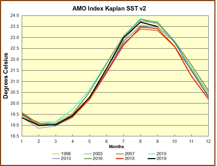
The UAH dataset includes temperature results for air above the oceans, and thus should be most comparable to the SSTs. There is the additional feature that ocean air temps avoid Urban Heat Islands (UHI). The graph below shows monthly anomalies for ocean temps since January 2015.
After a June rise in ocean air temps, all regions dropped back down to May levels in July and August. A spike occured in September, followed by plummenting October ocean air temps in the Tropics and SH. Now that drop has partly warmed back, leaving all regions in November slightly lower than September.
Land Air Temperatures Tracking Downward in Seesaw Pattern
We sometimes overlook that in climate temperature records, while the oceans are measured directly with SSTs, land temps are measured only indirectly. The land temperature records at surface stations sample air temps at 2 meters above ground. UAH gives tlt anomalies for air over land separately from ocean air temps. The graph updated for October is below. Here we have freash evidence of the greater volatility of the Land temperatures, along with an extraordinary departure by SH land. Despite the small amount of SH land, it spiked in July, then dropped in August so sharply along with the Tropics that it pulled the global average downward against slight warming in NH. Now again in November SH has jumped up beyond any month in this period. Despite this spike along with a rise in the Tropics, NH land temps dropped sharply. The larger NH land area pulled the Global average downward. The behavior of SH land temps is puzzling, to say the least.
The longer term picture from UAH is a return to the mean for the period starting with 1995:
TLTs include mixing above the oceans and probably some influence from nearby more volatile land temps. Clearly NH and Global land temps have been dropping in a seesaw pattern, more than 1C lower than the 2016 peak, prior to these last 2 months. TLT measures started the recent cooling later than SSTs from HadSST3, but are now showing the same pattern. It seems obvious that despite the three El Ninos, their warming has not persisted, and without them it would probably have cooled since 1995. Of course, the future has not yet been written.
Methane alarm is one of the moles continually popping up in the media Climate Whack-A-Mole game. An antidote to methane madness is now available to those inquiring minds who want to know reality without the hype.
Methane and Climate is a paper by W. A. van Wijngaarden (Department of Physics and Astronomy, York University, Canada) and W. Happer (Department of Physics, Princeton University, USA) published at CO2 Coalition November 22, 2019. It is a summary in advance of a more detailed publication to come. Excerpts in italics with my bolds.
Overview
Atmospheric methane (CH4) contributes to the radiative forcing of Earth’s atmosphere. Radiative forcing is the difference in the net upward thermal radiation from the Earth through a transparent atmosphere and radiation through an otherwise identical atmosphere with greenhouse gases. Radiative forcing, normally specified in units of W m−2 , depends on latitude, longitude and altitude, but it is often quoted for a representative temperate latitude, and for the altitude of the tropopause, or for the top of the atmosphere.
For current concentrations of greenhouse gases, the radiative forcing at the tropopause, per added CH4 molecule, is about 30 times larger than the forcing per added carbon-dioxide (CO2) molecule. This is due to the heavy saturation of the absorption band of the abundant greenhouse gas, CO2. But the rate of increase of CO2 molecules, about 2.3 ppm/year (ppm = part per million by mole), is about 300 times largerthan the rate of increase of CH4 molecules, which has been around 0.0076 ppm/year since the year 2008.
So the contribution of methane to the annual increase in forcing is one tenth (30/300) that of carbon dioxide. The net forcing increase from CH4 and CO2 increases is about 0.05 W m−2 year−1 . Other things being equal, this will cause a temperature increase of about 0.012 C year−1 . Proposals to place harsh restrictions on methane emissions because of warming fears are not justified by facts.
The paper is focused on the greenhouse effects of atmospheric methane, since there have recently been proposals to put harsh restrictions on any human activities that release methane. The basic radiation-transfer physicsoutlined in this paper gives no support to the idea that greenhouse gases like methane, CH4, carbon dioxide, CO2 or nitrous oxide, N2O are contributing to a climate crisis. Given the huge benefits of more CO2 to agriculture, to forestry, and to primary photosynthetic productivity in general, more CO2 is almost certainly benefitting the world. And radiative effects of CH4 and N2O, another greenhouse gas produced by human activities, are so small that they are irrelevant to climate.
Transmission of shortwave solar irradiation and long wavelength radiation from the Earth’s surface through atmosphere, as permitted by Rohde [2]. Note absorption wavelengths of CH4 are already covered by H2O and CO2.
Radiative Properties of Earth Atmosphere
On the left of Fig. 2 we have indicated the three most important atmospheric layers for radiative heat transfer. The lowest atmospheric layer is the troposphere, where parcels of air, warmed by contact with the solar-heated surface, float upward, much like hot-air balloons. As they expand into the surrounding air, the parcels do work at the expense of internal thermal energy. This causes the parcels to cool with increasing altitude, since heat flow in or out of parcels is usually slow compared to the velocities of ascent of descent.
Figure 2: Left. A standard atmospheric temperature profile[9], T = T (z). The surface temperature is T (0) = 288.7 K . Right. Standard concentrations[10], C {i} = N {i}/N for greenhouse molecules versus altitude z. The total number density of atmospheric molecules is N . At sea level the concentrations are 7750 ppm of H2O, 1.8 ppm of CH4 and 0.32 ppm of N2O. The O3 concentration peaks at 7.8 ppm at an altitude of 35 km, and the CO2 concentration was approximated by 400 ppm at all altitudes. The data is based on experimental observations.
If the parcels consisted of dry air, the cooling rate would be 9.8 C km−1 the dry adiabatic lapse rate[12]. But rising air has usually picked up water vapor from the land or ocean. The condensation of water vapor to droplets of liquid or to ice crystallites in clouds, releases so much latent heat that the lapse rates are less than 9.8 C km−1 in the lower troposphere. A representative lapse rate for mid latitudes is dT/dz = 6.5 K km−1 as shown in Fig. 2.
The tropospheric lapse rate is familiar to vacationers who leave hot areas near sea level for cool vacation homes at higher altitudesin the mountains. On average, the temperature lapse rates are small enough to keep the troposphere buoyantly stable[13]. Tropospheric air parcels that are displaced in altitude will oscillate up and down around their original position with periods of a few minutes. However, at any given time, large regions of the troposphere (particularly in the tropics) are unstable to moist convection because of exceptionally large temperature lapse rates.
The vertical radiation flux Z, which is discussed below, can change rapidly in the troposphere and stratosphere. There can be a further small change of Z in the mesosphere. Changes in Z above the mesopause are small enough to be neglected, so we will often refer to the mesopause as “the top of the atmosphere” (TOA), with respect to radiation transfer. As shown in Fig. 2, the most abundant greenhouse gas at the surface is water vapor, H2O. However, the concentration of water vapor drops by a factor of a thousand or more between the surface and the tropopause. This is because of condensation of water vapor into clouds and eventual removal by precipitation. Carbon dioxide, CO2, the most abundant greenhouse gas after water vapor, is also the most uniformly mixed because of its chemical stability.Methane, the main topic of this discussion is much less abundant than CO2 and it has somewhat higher concentrations in the troposphere than in the stratosphere where it is oxidized by OH radicals and ozone, O3. The oxidation of methane[8] is the main source of the stratospheric water vapor shown in Fig. 2.
Fluxes and Forcings
How greenhouse gases affect energy transfer through Earth’s atmosphere is quantitatively determined by the radiative forcing, F, the difference between the flux σT4 of thermal radiant energy from a black surface through a hypothetical, transparent atmosphere, and the flux Z through an atmosphere with greenhouse gases, particulates and clouds, but with the same surface temperature, T0.
Figure 3: Left: The altitude dependence of temperature from Fig. 2. Right The flux Z increases with increasing altitude as a result net upward energy radiation from the greenhouse gases H2O, O3, N2O and CH4, and CO2.
The forcing F and the flux Z are usually specified in units of W m−2. The radiative heating rate, dF R = , (3) dz is equal to the rate of change of the forcing with increasing altitude z. Over most of the atmosphere, R < 0, so thermal infrared radiation is a cooling mechanism that transfers internal energy of atmospheric molecules to space or to the Earth’s surface. Forcing depends on latitude, longitude and on the altitude, z. The right panel of Fig. 3 shows the altitude dependence of the net upward flux Z and the forcing F for the greenhouse gas concentrations of Fig. 2. The temperature profile of Fig 2 is reproduced in the left panel. The altitude-independent flux, σT 4 = 394 W m−2, from the surface with a temperature T0 = 288.7 K, through a hypothetical transparent atmosphere, is shown as the vertical dashed line in panel on the right. The fluxes for current concentrations of CO2 and for doubled or halved concentrations are shown as the continuous green line, the dashed red line and dotted blue line.
At current greenhouse gas concentrations the surface flux, 142 W m−2, is less than half the surface flux of 394 W m−2 for a transparent atmosphere because of downwelling radiation from greenhouse gases above. The surface flux has nearly doubled to 257 W m−2 at the tropopause altitude, 11 km in this example. The 115 W m−2 increase in flux from the surface to the tropopause has been radiated by greenhouse gases in the troposphere. Most of the energy needed to replace the radiated power comes from convection of moist air. Direct absorption of sunlight in the troposphere makes a much smaller contribution.
Spectral Forcings
Planck’s formula (7) for the spectral intensity of thermal radiation is one of the most famous equations of physics. It finally resolved the paradox that classical physics predicted infinite fluxes of heat radiation, in clear contradiction to observations, and it gave birth to quantum mechanics [16]. As one can see from Fig. 3, the flux at the top of the atmosphere, 277 W m−2 is only 70.3% of the flux σT 2 = 394 W m−2 emitted by a black surface at a temperature of T0 = 288.7 K. So without greenhouse gases, the surface would only need to radiate 70.3% of its current value to balance the same amount of solar heating. Since the Stefan-Boltzman flux is proportional to the fourth power of the surface temperature, without greenhouse gases the surface temperature could be smaller by a factor of (0.703)1/4 = 0.916. For this example, the greenhouse warming of the surface by all the greenhouse gases of Fig. 2 is ∆T = (1 0.916)T0 = 24.3 K. The warming would be different at different latitudes and longitudes, or in summer or winter, or if clouds are taken into account. But 20 C to 30 C is a reasonable estimate of how much warming is caused by current concentrations of greenhouse gases, compared to a completely transparent atmosphere.
Instantaneous forcing changes due to changes in the concentrations of greenhouse gases, but with no other changes to the atmosphere, can be calculated accurately for a given temperature profile. The next step, using instantaneous forcing changes to calculate temperature changes, is fraught with difficulties and is a major reason that climate models predict much more warming than observed[18]. As shown in Fig. 3, increasing the concentration of greenhouse gases (doubling the CO2 concentration for the example in the figure) slightly decreases the radiation flux through the atmosphere. In response, the atmosphere will slightly change − its properties to ensure that the average energy absorbed from sunlight is returned to space as thermal radiation. Since both the surface and greenhouse molecules radiate more intensely at higher temperatures, temperature increases are an obvious way to restore the equality of incoming and outgoing energy.
But the amount of water vapor and clouds in the atmosphere will also change, since water vapor is evaporated from the oceans and from moist land. Water is also precipitated from clouds as condensed rain or snow. Low, warm clouds reflect more sunlight and reduce solar heating, with little hindrance of thermal radiation to space. High, cold cirrus clouds reduce the thermal radiation to space, but are wispy and do little to hinder solar heating of the Earth.
The simplest response to changes in radiative forcing would be a uniform temperature increase dT , at every altitude and at the surface. The rate of increase of top-of-the atmosphere flux with a uniform temperature is then [1] dZ = 3.9 W m−2 K −1. (9) dT For a uniform temperature increase, the forcing increase ∆F = 0.23 W m−2 after 50 years, that would result if methane concentrations continued to rise at the rate of the previous 10 years as shown in Fig. 9, would cause a surface-temperature increase of ∆T = ∆F/(dZ/dT ) = 0.05 C. The forcing increase ∆F = 2.2 W m−2 after 50 years, if carbon dioxide concentrations continued to rise at the rate of the previous 10 years, would cause a surface-temperature increase of ∆T = ∆F/(dZ/dT ) = 0.59 C.
Both temperature increments are small and probably beneficial.
But there are persuasive reasons to expect that the temperature changes will be altitude dependent, like the forcing changes shown in Fig. 3, and that the water-vapor concentrations and cloud cover will change in response to changes in the surface temperature. Fig. 6 illustrates a more complicated “feedback” calculation.
Figure 6: Left. An initial temperature profile T (continuous blue line), the mid latitude profile of Fig. 3. The dashed red line is the adjusted temperature profile T ′ , after a doubling of the CO2 concentration. Right. The continuous blue line is the altitude profile of the “instantaneous” flux change ∆Z, caused by doubling CO2 concentrations.
On the left panel of Fig. 6, the continuous blue line labeled T is the midlatitude temperature profile of Fig. 3. The dashed red line labeled T ′ is the adjustment of the temperature profile in response to doubling the concentration of CO2, with a simultaneous increase in the concentration of water vapor in the troposphere The right panel of Fig. 6 summarizes forcing increments, with and without feedbacks. The continuous blue line is the instantaneous flux change from doubling CO2 concentrations, with no other changes to the atmosphere. It is the difference between the dashed red curve and the continuous green curve on the right of Fig. 3, but plotted on an expanded scale. The instantaneous forcing, ∆F = ∆Z, is 5.5 W m−2 at the tropopause altitude of 11 km, and 3.0 W m−2 at the 86 km altitude of the top of the atmosphere. The dashed red curve on the right of Fig. 6, labeled δZ is the “residual forcing” for the dashed-red temperature profile T ′ on the left, for doubled CO2 concentrations, and for the same relative humidity as before doubling CO2.
The same lapse rate, dT/dz = 6.5 K km−1, was used before and after doubling CO2 concentrations, as proposed by Manabe and Wetherald[19] in their model of “radiative-convective equilibrium.” This feedback prescription approximately doubles the surface warming, compared to a uniform temperature adjustment and no change in water vapor concentration. There is stratospheric cooling and surface warming. Variants of the radiative-convective equilibrium recipes illustrated in Fig. 6 are widely used in climate models. Unlike forcing calculations, which can be uniquely and reliably calculated, there is lots of room for subjective adjustments of the temperature changes caused by forcing changes.
Future Forcings of CH4 and CO2
Methane levels in Earth’s atmosphere are slowly increasing. If the current rate of increase, about 0.007 ppm/year for the past decade or so, were to continue unchanged it would take about 270 years to double the current concentration of C {i} = 1.8 ppm. But, as one can see from Fig.7, methane levels have stopped increasing for years at a time, so it is hard to be confident about future concentrations. Methane concentrations may never double, but if they do, WH[1] show that this would only increase the forcing by 0.8 W m−2. This is a tiny fraction of representative total forcings at midlatitudes of about 140 W m−2 at the tropopause and 120 W m−2 at the top of the atmosphere.
Figure 9: Projected mid-latitude forcing increments at the tropopause from continued increases of CO2 and CH4 at the rates of Fig. 7 and Fig. 8 for the next 50 years. The projected forcings are very small, especially for methane, compared to the current tropospheric forcing of 137 W m−2.
The per-molecule forcings P {i} of (13) and (14) have been used with the column density Nˆ of (12) and the concentration increase rates dC¯{i}/dt, noted in Fig. 7 and Fig. 8, to evaluate the future forcing (15), which is plotted in Fig. 9. Even after 50 years, the forcing increments from increased concentrations of methane (∆F = 0.23 W m−2), or the roughly ten times larger forcing from increased carbon dioxide (∆F = 2.2 W m−2) are very small compared to the total forcing, ∆F = 137 W m−2, shown in Fig. 3. The reason that the per-molecule forcing of methane is some 30 times larger than that of carbon dioxide for current concentrations is “saturation” of the absorption bands. The current density of CO2 molecules is some 200 times greater than that of CH4 molecules, so the absorption bands of CO2 are much more saturated than those of CH4. In the dilute“optically thin” limit, WH[1] show that the tropospheric forcing power per molecule is P {i} = 0.15 × 10⁻²² W for CH4, and P {i} = 2.73 × 10⁻²² W for CO2. Each CO2 molecule in the dilute limit causes about 5 times more forcing increase than an additional molecule of CH4, which is only a ”super greenhouse gas” because there is so little in the atmosphere, compared to CO2.
Dealing with alarmist claims is like playing whack-a-mole. Every time you beat down one bogeyman, another one pops up in another field, and later the first one returns, needing to be confronted again. I have been playing Climate Whack-A-Mole for a while, and if you are interested, there are some hammers supplied at the link above.
The alarmist methodology is repetitive, only the subject changes. First, create a computer model, purporting to be a physical or statistical representation of the real world. Then play with the parameters until fears are supported by the model outputs. Disregard or discount divergences from empirical observations. This pattern is described in more detail at Chameleon Climate Models
A series of posts apply reality filters to attest climate models.
The upcoming COP25 will be hosted by Chile, but held in Madrid because of the backlash in Santiago against damaging effects of costly climate policies. The gathering had been previously cancelled by a newly elected skeptical Brazilian president. The change of venue has led to “a scale down of expectations” and participation from the Chilean side, said Mónica Araya, a former lead negotiator for Costa Rica, but the presidency’s priorities are unchanged. In the wings of the Cop25 talks, hosts Spain and Chile will push governments to join a coalition of progressive nations pledging to raise their targets in response to the 2018 over-the-top IPCC SR15 climate horror movie. See UN Horror Show
Of course Spain is the setting for the adventures of Don Quixote ( “don key-ho-tee” ) in Cervantes’ famous novel. The somewhat factually challenged hero charged at some windmills claiming they were enemies, and is celebrated in the English language by two idioms:
Tilting at Windmills–meaning attacking imaginary enemies, and
Quixotic (“quick-sottic”)–meaning striving for visionary ideals.
It is clear that COP climateers are similary engaged in some kind of heroic quest, like modern-day Don Quixotes. The only differences: They imagine a trace gas in the air is the enemy, and that windmills are our saviors. See Climateers Tilting at Windmills
Four years ago French Mathematicians spoke out prior to COP21 in Paris, and their words provide a rational briefing for COP25 beginning in Madrid this weekend. In a nutshell:
Fighting Global Warming is Absurd, Costly and Pointless.
Absurd because of no reliable evidence that anything unusual is happening in our climate.
Costly because trillions of dollars are wasted on immature, inefficient technologies that serve only to make cheap, reliable energy expensive and intermittent.
Pointless because we do not control the weather anyway.
The prestigious Société de Calcul Mathématique (Society for Mathematical Calculation) issued a detailed 195-page White Paper that presents a blistering point-by-point critique of the key dogmas of global warming. The synopsis is blunt and extremely well documented. Here are extracts from the opening statements of the first three chapters of the SCM White Paper with my bolds and images.
Sisyphus at work.
Chapter 1: The crusade is absurd There is not a single fact, figure or observation that leads us to conclude that the world‘s climate is in any way ‘disturbed.’ It is variable, as it has always been, but rather less so now than during certain periods or geological eras. Modern methods are far from being able to accurately measure the planet‘s global temperature even today, so measurements made 50 or 100 years ago are even less reliable. Concentrations of CO2 vary, as they always have done; the figures that are being released are biased and dishonest. Rising sea levels are a normal phenomenon linked to upthrust buoyancy; they are nothing to do with so-called global warming. As for extreme weather events — they are no more frequent now than they have been in the past. We ourselves have processed the raw data on hurricanes….
Chapter 2: The crusade is costly Direct aid for industries that are completely unviable (such as photovoltaics and wind turbines) but presented as ‘virtuous’ runs into billions of euros, according to recent reports published by the Cour des Comptes (French Audit Office) in 2013. But the highest cost lies in the principle of ‘energy saving,’ which is presented as especially virtuous. Since no civilization can develop when it is saving energy, ours has stopped developing: France now has more than three million people unemployed — it is the price we have to pay for our virtue….
Chapter 3: The crusade is pointless Human beings cannot, in any event, change the climate. If we in France were to stop all industrial activity (let’s not talk about our intellectual activity, which ceased long ago), if we were to eradicate all trace of animal life, the composition of the atmosphere would not alter in any measurable, perceptible way. To explain this, let us make a comparison with the rotation of the planet: it is slowing down. To address that, we might be tempted to ask the entire population of China to run in an easterly direction. But, no matter how big China and its population are, this would have no measurable impact on the Earth‘s rotation.
Full text in pdf format is available in English at link below:
A Second report was published in 2016 entitled: Global Warming and Employment, which analyzes in depth the economic destruction from ill-advised climate change policies.
The two principal themes are that jobs are disappearing and that the destructive forces are embedded in our societies.
Jobs are Disappearing discusses issues such as:
The State is incapable of devising and implementing an industrial policy.
The fundamental absurdity of the concept of sustainable development
Biofuels an especially absurd policy leading to ridiculous taxes and job losses.
EU policy to reduce greenhouse gas emissions by 40% drives jobs elsewhere while being pointless: the planet has never asked for it, is completely unaware of it, and will never notice it!
The War against the Car and Road Maintenance undercuts economic mobility while destroying transportation sector jobs.
Solar and wind energy are weak, diffuse, and inconsistent, inadequate to power modern civilization.
Food production activities are attacked as being “bad for the planet.”
So-called Green jobs are entirely financed by subsidies.
The Brutalizing Whip discusses the damages to public finances and to social wealth and well-being, including these topics:
Taxes have never been so high
The Government is borrowing more and more
Dilapidated infrastructure
Instead of job creation, Relocations and Losses
The wastefulness associated with the new forms of energy
Return to the economy of an underdeveloped country
What is our predicament?
Four Horsemen are bringing down our societies:
The Ministry of Ecology (climate and environment);
Journalists;
Scientists;
Corporation Environmentalist Departments.
Steps required to recover from this demise:
Go back to the basic rules of research.
Go back to the basic rules of law
Do not trust international organizations
Leave the planet alone
Beware of any premature optimism
Conclusion
Climate lemmings
The real question is this: how have policymakers managed to make such absurd decisions, to blinker themselves to such a degree, when so many means of scientific investigation are available? The answer is simple: as soon as something is seen as being green, as being good for the planet, all discussion comes to an end and any scientific analysis becomes pointless or counterproductive. The policymakers will not listen to anyone or anything; they take all sorts of hasty, contradictory, damaging and absurd decisions. When will they finally be held to account?
Footnote:
The above cartoon image of climate talks includes water rising over politicians’ feet. But actual observations made in Fiji (presiding over 2017 talks in Bonn) show sea levels are stable (link below).
It is a valuable description of the temperature metrics and issues regarding climate analysis. They conclude:
None of the information on global temperatures is of any scientific value, and it should not
be used as a basis for any policy decisions. It is perfectly clear that:
there are far too few temperature sensors to give us a picture of the planet’s temperature;
we do not know what such a temperature might mean because nobody has given it
any specific physical significance;
the data have been subject to much dissimulation and manipulation. There is a
clear will not to mention anything that might be reassuring, and to highlight things
that are presented as worrying;
despite all this, direct use of the available figures does not indicate any genuine
trend towards global warming!
William Happer’s Major Statement at the Best Schools Global Warming Dialogue is CO₂ will be a major benefit to the Earth. Readers can learn much from the whole document (Title is link). Excerpts in italics with my bolds.
Some people claim that increased levels of atmospheric CO2 will cause catastrophic global warming, flooding from rising oceans, spreading tropical diseases, ocean acidification, and other horrors. But these frightening scenarios have almost no basis in genuine science. This Statement reviews facts that have persuaded me that more CO2 will be a major benefit to the Earth.
Discussions of climate today almost always involve fossil fuels. Some people claim that fossil fuels are inherently evil. Quite the contrary, the use of fossil fuels to power modern society gives the average person a standard of living that only the wealthiest could enjoy a few centuries ago. But fossil fuels must be extracted responsibly, minimizing environmental damage from mining and drilling operations, and with due consideration of costs and benefits. Similarly, fossil fuels must be burned responsibly, deploying cost-effective technologies that minimize emissions of real pollutants such as fly ash, carbon monoxide, oxides of sulfur and nitrogen, heavy metals, volatile organic compounds, etc.
Extremists have conflated these genuine environmental concerns with the emission of CO2, which cannot be economically removed from exhaust gases. Calling CO2 a “pollutant” that must be eliminated, with even more zeal than real pollutants, is Orwellian Newspeak.[3] “Buying insurance” against potential climate disasters by forcibly curtailing the use of fossil fuels is like buying “protection” from the mafia. There is nothing to insure against, except the threats of an increasingly totalitarian coalition of politicians, government bureaucrats, crony capitalists, thuggish nongovernmental organizations like Greenpeace, etc.
Figure 1. The ratio, RCO2, of past atmospheric CO2 concentrations to average values (about 300 ppm) of the past few million years, This particular proxy record comes from analyzing the fraction of the rare stable isotope 13C to the dominant isotope 12C in carbonate sediments and paleosols. Other proxies give qualitatively similar results.[
Life on Earth does better with more CO2. CO2 levels are increasing
Fig. 1 summarizes the most important theme of this discussion. It is not true that releasing more CO2 into the atmosphere is a dangerous, unprecedented experiment. The Earth has already “experimented” with much higher CO2 levels than we have today or that can be produced by the combustion of all economically recoverable fossil fuels.
Radiative cooling of the Earth and The Role of Water and Clouds
Without sunlight and only internal heat to keep warm, the Earth’s absolute surface temperature T would be very cold indeed. A first estimate can be made with the celebrated Stefan-Boltzmann formula
J= εσT^4 [Equation 1 ]
where J is the thermal radiation flux per unit of surface area, and the Stefan-Boltzmann constant (originally determined from experimental measurements) has the value σ = 5.67 × 10⁻⁸ W/(m2K4). If we use this equation to calculate how warm the surface would have to be to radiate the same thermal energy as the mean solar flux, Js = F/4 = 340 W/m2, we find Ts = 278 K or 5 C, a bit colder than the average temperature (287 K or 14 C) of the Earth’s surface,[19] but “in the ball park.”
Figure 5. The temperature profile of the Earth’s atmosphere.[20] This illustration is for mid-latitudes, like Princeton, NJ, at 40.4o N, where the tropopause is usually at an altitude of about 11 km. The tropopause is closer to 17 km near the equator, and as low as 9 km near the north and south poles.
These estimates can be refined by taking into account the Earth’s atmosphere. In the Interview we already discussed the representative temperature profile, Fig. 5. The famous “blue marble” photograph of the Earth,[21] reproduced in Fig. 6, is also very instructive. Much of the Earth is covered with clouds, which reflect about 30% of sunlight back into space, thereby preventing its absorption and conversion to heat. Rayleigh scattering (which gives the blue color of the daytime sky) also deflects shorter-wavelength sunlight back to space and prevents heating.
Today, whole-Earth images analogous to Fig. 6 are continuously recorded by geostationary satellites, orbiting at the same angular velocity as the Earth, and therefore hovering over nearly the same spot on the equator at an altitude of about 35,800 km.[23] In addition to visible images, which can only be recorded in daytime, the geostationary satellites record images of the thermal radiation emitted both day and night.
Figure 7. Radiation with wavelengths close to the 10.7 µ (1µ = 10-6m), as observed with a geostationary satellite over the western hemisphere of the Earth.[23] This is radiation in the infrared window of Fig. 4, where the surface can radiate directly to space from cloud-free regions.
Fig. 7 shows radiation with wavelengths close to 10.7 µ in the “infrared window” of the absorption spectrum shown in Fig. 4, where there is little absorption from either the main greenhouse gas, H2O, or from less-important CO2.Darker tones in Fig. 7 indicate more intense radiation. The cold “white” cloud tops emit much less radiation than the surface, which is “visible” at cloud-free regions of the Earth. This is the opposite from Fig. 6, where maximum reflected sunlight is coming from the white cloud tops, and much less reflection from the land and ocean, where much of the solar radiation is absorbed and converted to heat.
As one can surmise from Fig. 6 and Fig. 7, clouds are one of the most potent factors that control the surface temperature of the earth. Their effects are comparable to those of the greenhouse gases, H2O and CO2, but it is much harder to model the effects of clouds. Clouds tend to cool the Earth by scattering visible and near-visible solar radiation back to space before the radiation can be absorbed and converted to heat. But clouds also prevent the warm surface from radiating directly to space. Instead, the radiation comes from the cloud tops that are normally cooler than the surface. Low-cloud tops are not much cooler than the surface, so low clouds are net coolers. In Fig. 7, a large area of low clouds can be seen off the coast of Chile. They are only slightly cooler than the surrounding waters of the Pacific Ocean in cloud-free areas.
Figure 8. Spectrally resolved, vertical upwelling thermal radiation I from the Earth, the jagged lines, as observed by a satellite.[28] The smooth, dashed lines are theoretical Planck brightnesses, B, for various temperatures. The vertical units are 1 c.g.s = 1 erg/(s cm2 sr cm-1) = 1 mW/(m2 sr cm-1).
Except at the South Pole, the data of Fig. 8 show that the observed thermal radiation from the Earth is less intense than Planck radiation from the surface would be without greenhouse gases. Although the surface radiation is completely blocked in the bands of the greenhouse gases, as one would expect from Fig. 4, radiation from H2O and CO2 molecules at higher, colder altitudes can escape to space. At the “emission altitude,” which depends on frequency ν, there are not enough greenhouse molecules left overhead to block the escape of radiation. The thermal emission cross section of CO2 molecules at band center is so large that the few molecules in the relatively warm upper stratosphere (see Fig. 5) produce the sharp spikes in the center of the bands of Fig. 8. The flat bottoms of the CO2 bands of Fig 8 are emission from the nearly isothermal lower stratosphere (see Fig. 5) which has a temperature close to 220 K over most of the Earth.
It is hard for H2O molecules to reach cold, higher altitudes, since the molecules condense onto snowflakes or rain drops in clouds. So the H2O emissions to space come from the relatively warm and humid troposphere, and they are only moderately less intense than the Planck brightness of the surface. CO2 molecules radiate to space from the relatively dry and cold lower stratosphere. So for most latitudes, the CO2 band observed from space has much less intensity than the Planck brightness of the surface.
Concentrations of H2O vapor can be quite different at different locations on Earth. A good example is the bottom panel of Fig. 8, the thermal radiation from the Antarctic ice sheet, where almost no H2O emission can be seen. There, most of the water vapor has been frozen onto the ice cap, at a temperature of around 190 K. Near both the north and south poles there is a dramatic wintertime inversion[30] of the normal temperature profile of Fig. 5. The ice surface becomes much colder than most of the troposphere and lower stratosphere.
Cloud tops in the intertropical convergence zone (ITCZ) can reach the tropopause and can be almost as cold as the Antarctic ice sheet. The spectral distribution of cloud-top radiation from the ITCZ looks very similar to cloud-free radiation from the Antarctic ice, shown on the bottom panel of Fig. 8.
Convection
Radiation, which we have discussed above, is an important part of the energy transfer budget of the earth, but not the only part. More solar energy is absorbed in the tropics, near the equator, where the sun beats down nearly vertically at noon, than at the poles where the noontime sun is low on the horizon, even at midsummer, and where there is no sunlight at all in the winter. As a result, more visible and near infrared solar radiation (“short-wave radiation” or SWR) is absorbed in the tropics than is radiated back to space as thermal radiation (“long-wave radiation” or LWR). The opposite situation prevails near the poles, where thermal radiation releases more energy to space than is received by sunlight. Energy is conserved because the excess solar energy from the tropics is carried to the poles by warm air currents, and to a lesser extent, by warm ocean currents. The basic physics is sketched in Fig. 11.[35]
Figure 11. Most sunlight is absorbed in the tropics, and some of the heat energy is carried by air currents to the polar regions to be released back into space as thermal radiation. Along with energy, angular momentum — imparted to the air from the rotating Earth’s surface near the equator — is transported to higher northern and southern latitudes, where it is reabsorbed by the Earth’s surface. The Hadley circulation near the equator is largely driven by buoyant forces on warm, solar-heated air, but for mid latitudes the “Coriolis force” due to the rotation of the earth leads to transport of energy and angular momentum through slanted “baroclinic eddies.” Among other consequences of the conservation of angular momentum are the easterly trade winds near the equator and the westerly winds at mid latitudes.
Equilibrium Climate Sensitivity
If increasing CO2 causes very large warming, harm can indeed be done. But most studies suggest that warmings of up to 2 K will be good for the planet,[38] extending growing seasons, cutting winter heating bills, etc. We will denote temperature differences in Kelvin (K) since they are exactly the same as differences in Celsius (C). A temperature change of 1 K = 1 C is equal to a change of 1.8 Fahrenheit (F).
If a 50% increase of CO2 were to increase the temperature by 3.4 K, as in Arrhenius’s original estimate mentioned above, the doubling sensitivity would be S = 3.4 K/log2(1.5) = 5.8 K. Ten years later, on page 53 of his popular book, Worlds in the Making: The Evolution of the Universe,[40] Arrhenius again states the logarithmic law of warming, with a slightly smaller climate sensitivity, S = 4 K.
Convection of the atmosphere, water vapor, and clouds all interact in a complicated way with the change of CO2 to give the numerical value of the doubling sensitivity S of Eq. (21). Remarkably, Arrhenius somehow guessed the logarithmic dependence on CO2 concentration before Planck’s discovery of how thermal radiation really works.
More than a century after Arrhenius, and after the expenditure of many tens of billions of dollars on climate science, the official value of S still differs little from the guess that Arrhenius made in 1912: S = 4 K.
Could it be that the climate establishment does not want to work itself out of a job?
Overestimate of Sensitivity
Contrary to the predictions of most climate models, there has been very little warming of the Earth’s surface over the last two decades. The discrepancy between models and observations issummarized by Fyfe, Gillett, and Zwiers, as shown in the Fyfe Fig.1 above.
At this writing, more than 50 mechanisms have been proposed to explain the discrepancy of Fyfe Fig.1. These range from aerosol cooling to heat absorption by the ocean. Some of the more popular excuses for the discrepancy have been summarized by Fyfe, et al. But the most straightforward explanation for the discrepancy between observations and models is that the doubling sensitivity, which most models assume to be close to the “most likely” IPCC value, S = 3 K, is much too large.
If one assumes negligible feedback, where other properties of the atmosphere change little in response to additions of CO2, the doubling efficiency can be estimated to be about S = 1 K, for example, as we discussed in connection with Eq. (19). The much larger doubling sensitivities claimed by the IPCC, which look increasingly dubious with each passing year, are due to “positive feedbacks.” A favorite positive feedback is the assumption that water vapor will be lofted to higher, colder altitudes by the addition of more CO2, thereby increasing the effective opacity of the vapor. Changes in cloudiness can also provide either positive feedback which increases S or negative feedback which decreases S. The simplest interpretation of the discrepancy of Fig. 13 and Fig. 14 is that the net feedback is small and possibly even negative. Recent work by Harde indicates a doubling sensitivity of S = 0.6 K.[46]
Figure 17. The analysis of satellite observations by Dr. Randall J. Donohohue and co-workers[53] shows a clear greening of the earth from the modest increase of CO2 concentrations from about 340 ppm to 400 ppm from the year 1982 to 2010. The greening is most pronounced in arid areas where increased CO2 levels diminish the water requirement of plants.
Benefits of CO2
More CO2 in the atmosphere will be good for life on planet earth. Few realize that the world has been in a CO2 famine for millions of years — a long time for us, but a passing moment in geological history. Over the past 550 million years since the Cambrian, when abundant fossils first appeared in the sedimentary record, CO2 levels have averaged many thousands of parts per million (ppm), not today’s few hundred ppm, which is not that far above the minimum level, around 150 ppm, when many plants die of CO2 starvation.
All green plants grow faster with more atmospheric CO2. It is found that the growth rate is approximately proportional to the square root of the CO2 concentrations, so the increase in CO2 concentrations from about 300 ppm to 400 ppm over the past century should have increased growth rates by a factor of about √(4/3) = 1.15, or 15%. Most crop yields have increased by much more than 15% over the past century. Better crop varieties, better use of fertilizer, better water management, etc., have all contributed. But the fact remains that a substantial part of the increase is due to more atmospheric CO2.
But the nutritional value of additional CO2 is only part of its benefit to plants. Of equal or greater importance, more CO2 in the atmosphere makes plants more drought-resistant. Plant leaves are perforated by stomata, little holes in the gas-tight surface skin that allow CO2 molecules to diffuse from the outside atmosphere into the moist interior of the leaf where they are photosynthesized into carbohydrates.
In the course of evolution, land plants have developed finely tuned feedback mechanisms that allow them to grow leaves with more stomata in air that is poor in CO2, like today, or with fewer stomata for air that is richer in CO2, as has been the case over most of the geological history of land plants.[51] If the amount of CO2 doubles in the atmosphere, plants reduce the number of stomata in newly grown leaves by about a factor of two. With half as many stomata to leak water vapor, plants need about half as much water. Satellite observations like those of Fig. 17 from R.J. Donohue, et al.,[52] have shown a very pronounced “greening” of the Earth as plants have responded to the modest increase of CO2 from about 340 ppm to 400 ppm during the satellite era. More greening and greater agricultural yields can be expected as CO2 concentrations increase further.
Climate Science
Droughts, floods, heat waves, cold snaps, hurricanes, tornadoes, blizzards, and other weather- and climate-related events will complicate our life on Earth, no matter how many laws governments pass to “stop climate change.” But if we understand these phenomena, and are able to predict them, they will be much less damaging to human society. So I strongly support high-quality research on climate and related fields like oceanography, geology, solar physics, etc. Especially important are good measurement programs like the various satellite measurements of atmospheric temperature[59] or the Argo[60] system of floating buoys that is revolutionizing our understanding of ocean currents, temperature, salinity, and other important properties.
But too much “climate research” money is pouring into very questionable efforts, like mitigation of the made-up horrors mentioned above. It reminds me of Gresham’s Law: “Bad money drives out good.”[61] The torrent of money showered on scientists willing to provide rationales, however shoddy, for the war on fossil fuels, and cockamamie mitigation schemes for non-existent problems, has left insufficient funding for honest climate science.
Summary
The Earth is in no danger from increasing levels of CO2. More CO2 will be a major benefit to the biosphere and to humanity. Some of the reasons are:
As shown in Fig. 1, much higher CO2 levels than today’s prevailed over most last 550 million years of higher life forms on Earth. Geological history shows that the biosphere does better with more CO2.
As shown in Fig. 13 and Fig. 14, observations over the past two decades show that the warming predicted by climate models has been greatly exaggerated. The temperature increase for doubling CO2 levels appears to be close to the feedback-free doubling sensitivity of S =1 K, and much less than the “most likely” value S = 3 K promoted by the IPCC and assumed in most climate models.
As shown in Fig. 12, if CO2 emissions continue at levels comparable to those today, centuries will be needed for the added CO2 to warm the Earth’s surface by 2 K, generally considered to be a safe and even beneficial amount.
Over the past tens of millions of years, the Earth has been in a CO2 famine with respect to the optimal levels for plants, the levels that have prevailed over most of the geological history of land plants. There was probably CO2 starvation of some plants during the coldest periods of recent ice ages. As shown in Fig. 15–17, more atmospheric CO2 will substantially increase plant growth rates and drought resistance.
There is no reason to limit the use of fossil fuels because they release CO2 to the atmosphere. However, fossil fuels do need to be mined, transported, and burned with cost-effective controls of real environmental problems — for example, fly ash, oxides of sulfur and nitrogen, volatile organic compounds, groundwater contamination, etc.
Sometime in the future, perhaps by the year 2050 when most of the original climate crusaders will have passed away, historians will write learned papers on how it was possible for a seemingly enlightened civilization of the early 21st century to demonize CO2, much as the most “Godly” members of society executed unfortunate “witches” in earlier centuries.
Dr. William Happer Background: Co-Founder and current Director of the CO2 Coalition, Dr. William Happer, Professor Emeritus in the Department of Physics at Princeton University, is a specialist in modern optics, optical and radiofrequency spectroscopy of atoms and molecules, radiation propagation in the atmosphere, and spin-polarized atoms and nuclei.
From September 2018 to September 2019, Dr. Happer served as Deputy Assistant to the President and Senior Director of Emerging Technologies on the National Security Council.
He has published over 200 peer-reviewed scientific papers. He is a Fellow of the American Physical Society, the American Association for the Advancement of Science, and a member of the American Academy of Arts and Sciences, the National Academy of Sciences and the American Philosophical Society. He was awarded an Alfred P. Sloan Fellowship in 1966, an Alexander von Humboldt Award in 1976, the 1997 Broida Prize and the 1999 Davisson-Germer Prize of the American Physical Society, and the Thomas Alva Edison Patent Award in 2000.
Simulation of jet stream pattern July 22. (VentuSky.com)
We are heading into winter this year at the bottom of a solar cycle, and ocean oscillations due for cooling phases. The folks at Climate Alarm Central (CAC) are well aware of this, and are working hard so people won’t realize that global cooling contradicts global warming. No indeed, contortionist papers and headlines are warning us all that CO2 not only causes hothouse earth, overrun with rats and other vermin. CO2 also causes ice ages when it feels like it.
The jet has always varied – and has always affected our weather patterns. But now climate change is affecting our weather too. As I explore in my latest book, it’s when the wanderings of the jet and the hand of climate change add up that we get record-breaking heatwaves, floods and droughts – but not freezes.
In many ways, the summer of 2018 marked a turning point, when the effects of climate change — perhaps previously on the periphery of public consciousness — suddenly took center stage. Record high temperatures spread all over the Northern Hemisphere. Wildfires raged out of control. And devastating floods were frequent.
Michael Mann, climate scientist at Pennsylvania State University, along with colleagues, has published a new study that connects these disruptive weather extremes with a fundamental change in how the jet stream is behaving during the summer. Linked to the warming climate, the study suggests this change in the atmosphere’s steering current is making these extremes occur more frequently, with greater intensity, and for longer periods of time.
The study projects this erratic jet-stream behavior will increase in the future, leading to more severe heat waves, droughts, fires and floods.
The jet stream is changing not only because the planet is warming up but also because the Arctic is warming faster than the mid-latitudes, the study says. The jet stream is driven by temperature contrasts, and these contrasts are shrinking. The result is a slower jet stream with more wavy peaks and troughs that Mann and his study co-authors ascribe to a process known as “quasi-resonant amplification.”
The altered jet-stream behavior is important because when it takes deep excursions to the south in the summer, it sets up a collision between cool air from the north and the summer’s torrid heat, often spurring excessive rain. But when the jet stream retreats to the north, bulging heat domes form underneath it, leading to record heat and dry spells.
The study, published Wednesday in Science Advances, finds that these quasi-resonant amplification events — in which the jet stream exhibits this extreme behavior during the summer — are predicted to increase by 50 percent this century if emissions of carbon dioxide and other greenhouse gases continue unchecked.
Whereas previous work conducted by Mann and others had identified a signal for an increase in these events, this study for the first time examined how they may change in the future using climate model simulations.
“Looking at a large number of different computer models, we found interesting differences,” said Stefan Rahmstorf from the Potsdam Institute for Climate Impact Research and a co-author of the study, in a news release. “Distinct climate models provide quite diverging forecasts for future climate resonance events. However, on average they show a clear increase in such events.”
Although model projections suggest these extreme jet-stream patterns will increase as the climate warms, the study concluded that their increase can be slowed if greenhouse gas emissions are reduced along with particulate pollution in developing countries. “[T]he future is still very much in our hands when it comes to dangerous and damaging summer weather extremes,” Mann said. “It’s simply a matter of our willpower to transition quickly from fossil fuels to renewable energy.”
Mann has been leading the charge to blame anticipated cooling on fossil fuels, his previous attempt claiming CO2 is causing a slowdown of AMOC (part of it being the Gulf Stream), resulting in global cooling, even an ice age. The same idea underlay the scary 2004 movie Day After Tomorrow.
Indices of subsurface temperature, sea surface height (SSH), latent heat flux (LHF), and sea surface temperature (SST). SST (purple) is plotted using the same scale as subsurface temperature (blue) in the upper panel. The upper panel shows 24 month filtered values of de‐seasonalized anomalies along with the non‐Ekman part of the AMOC. In the lower panel, we show three‐year running means of the indices going back to 1985 (1993 for the SSH index).
Changes in ocean heat transport and SST are expected to modify the net air‐sea heat flux. The changes in the total air‐sea flux (Figure S4, data obtained from the National Centers for Environmental Prediction‐National Center for Atmospheric Research reanalysis; Kalnay et al., 1996) are almost all due to the change in LHF. The third panel of Figure 3 shows the changes in LHF between the two periods. There is a strong signal with increased heat loss from the ocean over the Gulf Stream. That the area of increased heat loss coincides with the location of warming SST indicates that the changes in air‐sea fluxes are driven by the ocean.
Whilst the AMOC has only been continuously measured since 2004, the indices of SSH, heat content, SST, and LHF can be calculated farther back in time (Figure 3, bottom). Over this longer time period, all four indices are strongly correlated with one another (Table S5; correlations were calculated using the nonparametric method described in McCarthy et al., 2015). These data suggest that measurement of the AMOC at 26°N started close to a maximum in the overturning. Prior to 2007 the indices show variability on a time scale of 8 to 10 years and no trend is evident, but since 2014 all indices have had values lower than any other year since 1985.
Previous studies have shown that seasonal and interannual changes in the subtropical AMOC are forced primarily by changing wind stress mediated by Rossby waves (Zhao & Johns, 2014a, 2014b). There is growing evidence (Delworth et al., 2016; Jackson et al., 2016) that the longer‐term changes of the AMOC over the last decade are also associated with thermohaline forcing and that the changed circulation alters the pattern of ocean‐atmosphere heat exchange (Gulev et al., 2013). The role of ocean circulation in decadal climate variability has been challenged in recent years with authors suggesting that external, atmospheric‐driven changes could produce the observed variability in Atlantic SSTs (Clement et al., 2015). However, the direct observation of a weakened AMOC supports a role for ocean circulation in decadal Atlantic climate variability.
Our results show that the previously reported decline of the AMOC (Smeed et al., 2014) has been arrested, but the length of the observational record of the AMOC is still short relative to the time scales of important decadal variations that exist in the Atlantic. Understanding is therefore constantly evolving. What we identify as a changed state of the AMOC in this study may well prove to be part of a decadal oscillation superposed on a multidecadal cycle. Overlaying these oscillations is the impact of anthropogenic change that is predicted to weaken the AMOC over the next century. The continuation of measurements from the RAPID 26°N array and similar observations elsewhere in the Atlantic (Lozier et al., 2017; Meinen et al., 2013) will enable us to unravel and reveal the role of ocean circulation in the changing Atlantic climate in the coming decades.
Regarding the more recent attempt to link CO2 with jet stream meanderings, we have this paper providing a more reasonable assessment. Arctic amplification: does it impact the polar jet stream? by Valentin P. Meleshko et al. Excerpts below in italics with my bolds.
Analysis of observation and model simulations has revealed that northward temperature gradient decreases and jet flow weakens in the polar troposphere due to global climate warming. These interdependent phenomena are regarded as robust features of the climate system. An increase of planetary wave oscillation that is attributed to Arctic amplification (Francis and Vavrus, 2012; Francis and Vavrus, 2015) has not been confirmed from analysis of observation (Barnes, 2013; Screen and Simmonds, 2013) or in our analysis of model simulations of projected climate. However, we found that GPH variability associated with planetary wave oscillation increases in the background of weakening of zonal flow during the sea-ice-free summer. Enhancement of northward heat transport in the troposphere was shown to be the main factor responsible for decrease of northward temperature gradient and weakening of the jet stream in autumn and winter. Arctic amplification provides only minor contribution to the evolution of zonal flow and planetary wave oscillation.
It has been shown that northward heat transport is the major factor in decreasing the northward temperature gradient in the polar atmosphere and increasing the planetary-scale wave oscillation in the troposphere of the mid-latitudes. Arctic amplification does not show any essential impact on planetary-scale oscillation in the mid and upper troposphere, although it does cause a decrease of northward heat transport in the lower troposphere. These results confound the interpretation of the short observational record that has suggested a causal link between recent Arctic melting and extreme weather in the mid-latitudes.
There are two additional explanations of factors causing the wavy jet stream, AKA Polar Vortex. Dr Judah Cohen of AER has written extensively on the link between Autumn Siberian snow cover and the Arctic oscillation. See Snowing and Freezing in the Arcticfor a more complete description of the mechanism.
Finally, a discussion with Piers Corbyn regarding the solar flux effect upon the jet stream at Is This Cold the New Normal?
Figure: Global Hurricane Frequency (all & major) — 12-month running sums. The top time series is the number of global tropical cyclones that reached at least hurricane-force (maximum lifetime wind speed exceeds 64-knots). The bottom time series is the number of global tropical cyclones that reached major hurricane strength (96-knots+). Adapted from Maue (2011) GRL.
This post refers to statistics for this year’s Atlantic and Global Hurricane season, now likely completed. The chart above was updated by Ryan Maue yesterday. A detailed report is provided by the Colorado State University Tropical Meteorology Project, directed by Dr. William Gray until his death in 2016. More from Bill Gray in a reprinted post at the end.
The 2019 Atlantic hurricane season was slightly above average and had a little more activity than what was predicted by our June-August updates. The climatological peak months of the hurricane season were characterized by a below-average August, a very active September, and above-average named storm activity but below-average hurricane activity in October. Hurricane Dorian was the most impactful hurricane of 2019, devastating the northwestern Bahamas before bringing significant impacts to the
southeastern United States and the Atlantic Provinces of Canada. Tropical Storm Imelda also brought significant flooding to southeast Texas.
Open image in new tab to enlarge.
The 2019 hurricane season overall was slightly above average. The season was characterized by an above-average number of named storms and a near-average number of hurricanes and major hurricanes. Our initial seasonal forecast issued in April somewhat underestimated activity, while seasonal updates issued in June, July and August, respectively, slightly underestimated overall activity. The primary reason for the underestimate was due to a more rapid abatement of weak El Niño conditions than was originally anticipated. August was a relatively quiet month for Atlantic TC activity, while September was well above-average. While October had an above-average number of named storm formations, overall Accumulated Cyclone Energy was slightly below normal.
Figure: Last 4-decades of Global and Northern Hemisphere Accumulated Cyclone Energy: 24 month running sums. Note that the year indicated represents the value of ACE through the previous 24-months for the Northern Hemisphere (bottom line/gray boxes) and the entire global (top line/blue boxes). The area in between represents the Southern Hemisphere total ACE.
Previous Post: Bill Gray: H20 is Climate Control Knob, not CO2
William Mason Gray (1929-2016), pioneering hurricane scientist and forecaster and professor of atmospheric science at Colorado State University.
Dr. William Gray made a compelling case for H2O as the climate thermostat, prior to his death in 2016. Thanks to GWPF for publishing posthumously Bill Gray’s understanding of global warming/climate change. The paper was compiled at his request, completed and now available as Flaws in applying greenhouse warming to Climate Variability This post provides some excerpts in italics with my bolds and some headers. Readers will learn much from the entire document (title above is link to pdf).
The Fundamental Correction
The critical argument that is made by many in the global climate modeling (GCM) community is that an increase in CO2 warming leads to an increase in atmospheric water vapor, resulting in more warming from the absorption of outgoing infrared radiation (IR) by the water vapor. Water vapor is the most potent greenhouse gas present in the atmosphere in large quantities. Its variability (i.e. global cloudiness) is not handled adequately in GCMs in my view. In contrast to the positive feedback between CO2 and water vapor predicted by the GCMs, it is my hypothesis that there is a negative feedback between CO2 warming and and water vapor. CO2 warming ultimately results in less water vapor (not more) in the upper troposphere. The GCMs therefore predict unrealistic warming of global temperature. I hypothesize that the Earth’s energy balance is regulated by precipitation (primarily via deep cumulonimbus (Cb) convection) and that this precipitation counteracts warming due to CO2.
Figure 14: Global surface temperature change since 1880. The dotted blue and dotted red lines illustrate how much error one would have made by extrapolating a multi-decadal cooling or warming trend beyond a typical 25-35 year period. Note the recent 1975-2000 warming trend has not continued, and the global temperature remained relatively constant until 2014.
Projected Climate Changes from Rising CO2 Not Observed
Continuous measurements of atmospheric CO2, which were first made at Mauna Loa, Hawaii in 1958, show that atmospheric concentrations of CO2 have risen since that time. The warming influence of CO2 increases with the natural logarithm (ln) of the atmosphere’s CO2 concentration. With CO2 concentrations now exceeding 400 parts per million by volume (ppm), the Earth’s atmosphere is slightly more than halfway to containing double the 280 ppm CO2 amounts in 1860 (at the beginning of the Industrial Revolution).∗
We have not observed the global climate change we would have expected to take place, given this increase in CO2. Assuming that there has been at least an average of 1 W/m2 CO2 blockage of IR energy to space over the last 50 years and that this energy imbalance has been allowed to independently accumulate and cause climate change over this period with no compensating response, it would have had the potential to bring about changes in any one of the following global conditions:
Warm the atmosphere by 180◦C if all CO2 energy gain was utilized for this purpose – actual warming over this period has been about 0.5◦C, or many hundreds of times less.
Warm the top 100 meters of the globe’s oceans by over 5◦C – actual warming over this period has been about 0.5◦C, or 10 or more times less.
Melt sufficient land-based snow and ice as to raise the global sea level by about 6.4 m. The actual rise has been about 8–9 cm, or 60–70 times less. The gradual rise of sea level has been only slightly greater over the last ~50 years (1965–2015) than it has been over the previous two ~50-year periods of 1915–1965 and 1865–1915, when atmospheric CO2 gain was much less.
Increase global rainfall over the past ~50-year period by 60 cm.
Earth Climate System Compensates for CO2
If CO2 gain is the only influence on climate variability, large and important counterbalancing influences must have occurred over the last 50 years in order to negate most of the climate change expected from CO2’s energy addition. Similarly, this hypothesized CO2-induced energy gain of 1 W/m2 over 50 years must have stimulated a compensating response that acted to largely negate energy gains from the increase in CO2.
The continuous balancing of global average in-and-out net radiation flux is therefore much larger than the radiation flux from anthropogenic CO2. For example, 342 W/m2, the total energy budget, is almost 100 times larger than the amount of radiation blockage expected from a CO2 doubling over 150 years. If all other factors are held constant, a doubling of CO2 requires a warming of the globe of about 1◦C to enhance outward IR flux by 3.7 W/m2 and thus balance the blockage of IR flux to space.
Figure 2: Vertical cross-section of the annual global energy budget. Determined from a combination of satellite-derived radiation measurements and reanalysis data over the period of 1984–2004.
This pure IR energy blocking by CO2 versus compensating temperature increase for radiation equilibrium is unrealistic for the long-term and slow CO2 increases that are occurring. Only half of the blockage of 3.7 W/m2 at the surface should be expected to go into an temperature increase.The other half (about 1.85 W/m2) of the blocked IR energy to space will be compensated by surface energy loss to support enhanced evaporation. This occurs in a similar way to how the Earth’s surface energy budget compensates for half its solar gain of 171 W/m2 by surface-to-air upward water vapor flux due to evaporation.
Assuming that the imposed extra CO2 doubling IR blockage of 3.7 W/m2 is taken up and balanced by the Earth’s surface in the same way as the solar absorption is taken up and balanced, we should expect a direct warming of only ~0.5◦C for a doubling of CO2. The 1◦C expected warming that is commonly accepted incorrectly assumes that all the absorbed IR goes to the balancing outward radiation with no energy going to evaporation.
Consensus Science Exaggerates Humidity and Temperature Effects
A major premise of the GCMs has been their application of the National Academy of Science (NAS) 1979 study3 – often referred to as the Charney Report – which hypothesized that a doubling of atmospheric CO2 would bring about a general warming of the globe’s mean temperature of 1.5–4.5◦C (or an average of ~3.0◦C). These large warming values were based on the report’s assumption that the relative humidity (RH) of the atmosphere remains quasiconstant as the globe’s temperature increases. This assumption was made without any type of cumulus convective cloud model and was based solely on the Clausius–Clapeyron (CC) equation and the assumption that the RH of the air will remain constant during any future CO2-induced temperature changes. If RH remains constant as atmospheric temperature increases, then the water vapor content in the atmosphere must rise exponentially.
With constant RH, the water vapor content of the atmosphere rises by about 50% if atmospheric temperature is increased by 5◦C. Upper tropospheric water vapor increases act to raise the atmosphere’s radiation emission level to a higher and thus colder level. This reduces the amount of outgoing IR energy which can escape to space by decreasing T^4.
These model predictions of large upper-level tropospheric moisture increases have persisted in the current generation of GCM forecasts.§ These models significantly overestimate globally-averaged tropospheric and lower stratospheric (0–50,000 feet) temperature trends since 1979 (Figure 7).
Figure 8: Decline in upper tropospheric RH. Annually-averaged 300 mb relative humidity for the tropics (30°S–30°N). From NASA-MERRA2 reanalysis for 1980–2016. Black dotted line is linear trend.
All of these early GCM simulations were destined to give unrealistically large upper-tropospheric water vapor increases for doubling of CO2 blockage of IR energy to space, and as a result large and unrealistic upper tropospheric temperature increases were predicted. In fact, if data from NASA-MERRA24 and NCEP/NCAR5 can be believed, upper tropospheric RH has actually been declining since 1980 as shown in Figure 8. The top part of Table 1 shows temperature and humidity differences between very wet and dry years in the tropics since 1948; in the wettest years, precipitation was 3.9% higher than in the driest ones. Clearly, when it rains more in the tropics, relative and specific humidity decrease. A similar decrease is seen when differencing 1995–2004 from 1985–1994, periods for which the equivalent precipitation difference is 2%. Such a decrease in RH would lead to a decrease in the height of the radiation emission level and an increase in IR to space.
The Earth’s natural thermostat – evaporation and precipitation
What has prevented this extra CO2-induced energy input of the last 50 years from being realized in more climate warming than has actually occurred? Why was there recently a pause in global warming, lasting for about 15 years? The compensating influence that prevents the predicted CO2-induced warming is enhanced global surface evaporation and increased precipitation.
Annual average global evaporational cooling is about 80 W/m2 or about 2.8 mm per day. A little more than 1% extra global average evaporation per year would amount to 1.3 cm per year or 65 cm of extra evaporation integrated over the last 50 years. This is the only way that such a CO2-induced , 1 W/m2 IR energy gain sustained over 50 years could occur without a significant alteration of globally-averaged surface temperature. This hypothesized increase in global surface evaporation as a response to CO2-forced energy gain should not be considered unusual. All geophysical systems attempt to adapt to imposed energy forcings by developing responses that counter the imposed action. In analysing the Earth’s radiation budget, it is incorrect to simply add or subtract energy sources or sinks to the global system and expect the resulting global temperatures to proportionally change. This is because the majority of CO2-induced energy gains will not go into warming the atmosphere. Various amounts of CO2-forced energy will go into ocean surface storage or into ocean energy gain for increased surface evaporation.Therefore a significant part of the CO2 buildup (~75%) will bring about the phase change of surface liquid water to atmospheric water vapour. The energy for this phase change must come from the surface water, with an expenditure of around 580 calories of energy for every gram of liquid that is converted into vapour. The surface water must thus undergo a cooling to accomplish this phase change.
Therefore, increases in anthropogenic CO2 have brought about a small (about 0.8%) speeding up of the globe’s hydrologic cycle, leading to more precipitation, and to relatively little global temperature increase. Therefore, greenhouse gases are indeed playing an important role in altering the globe’s climate, but they are doing so primarily by increasing the speed of the hydrologic cycle as opposed to increasing global temperature. Figure 9: Two contrasting views of the effects of how the continuous intensification of deep
cumulus convection would act to alter radiation flux to space.
The top (bottom) diagram represents a net increase (decrease) in radiation to space
Tropical Clouds Energy Control Mechanism
It is my hypothesis that the increase in global precipitation primarily arises from an increase in deep tropical cumulonimbus (Cb) convection. The typical enhancement of rainfall and updraft motion in these areas together act to increase the return flow mass subsidence in the surrounding broader clear and partly cloudy regions. The upper diagram in Figure 9 illustrates the increasing extra mass flow return subsidence associated with increasing depth and intensity of cumulus convection. Rainfall increases typically cause an overall reduction of specific humidity (q) and relative humidity (RH) in the upper tropospheric levels of the broader scale surrounding convective subsidence regions. This leads to a net enhancement of radiation flux to space due to a lowering of the upper-level emission level. This viewpoint contrasts with the position in GCMs, which suggest that an increase in deep convection will increase upper-level water vapour.
Figure 10: Conceptual model of typical variations of IR, albedo and net (IR + albedo) associated with three different areas of rain and cloud for periods of increased precipitation.
The albedo enhancement over the cloud–rain areas tends to increase the net (IR + albedo) radiation energy to space more than the weak suppression of (IR + albedo) in the clear areas. Near-neutral conditions prevail in the partly cloudy areas. The bottom diagram of Figure 9 illustrates how, in GCMs, Cb convection erroneously increases upper tropospheric moisture. Based on reanalysis data (Table 1, Figure 8) this is not observed in the real atmosphere.
Ocean Overturning Circulation Drives Warming Last Century
A slowing down of the global ocean’s MOC is the likely cause of most of the global warming that has been observed since the latter part of the 19th century.15 I hypothesize that shorter multi-decadal changes in the MOC16 are responsible for the more recent global warming periods between 1910–1940 and 1975–1998 and the global warming hiatus periods between 1945–1975 and 2000–2013.
Figure 12: The effect of strong and weak Atlantic THC. Idealized portrayal of the primary Atlantic Ocean upper ocean currents during strong and weak phases of the thermohaline circulation (THC)
Figure 13 shows the circulation features that typically accompany periods when the MOC is stronger than normal and when it is weaker than normal. In general, a strong MOC is associated with a warmer-than-normal North Atlantic, increased Atlantic hurricane activity, increased blocking action in both the North Atlantic and North Pacific and weaker westerlies in the mid-latitude Southern Hemisphere. There is more upwelling of cold water in the South Pacific and Indian Oceans, and an increase in global rainfall of a few percent occurs. This causes the global surface temperatures to cool. The opposite occurs when the MOC is weaker than normal.
The average strength of the MOC over the last 150 years has likely been below the multimillennium average, and that is the primary reason we have seen this long-term global warming since the late 19th century. The globe appears to be rebounding from the conditions of the Little Ice Age to conditions that were typical of the earlier ‘Medieval’ and ‘Roman’ warm periods.
Summary and Conclusions
The Earth is covered with 71% liquid water. Over the ocean surface, sub-saturated winds blow, forcing continuous surface evaporation. Observations and energy budget analyses indicate that the surface of the globe is losing about 80 W/m2 of energy from the global surface evaporation process. This evaporation energy loss is needed as part of the process of balancing the surface’s absorption of large amounts of incoming solar energy. Variations in the strength of the globe’s hydrologic cycle are the way that the global climate is regulated. The stronger the hydrologic cycle, the more surface evaporation cooling occurs, and greater the globe’s IR flux to space. The globe’s surface cools when the hydrologic cycle is stronger than average and warms when the hydrologic cycle is weaker than normal. The strength of the hydrologic cycle is thus the primary regulator of the globe’s surface temperature. Variations in global precipitation are linked to long-term changes in the MOC (or THC).
I have proposed that any additional warming from an increase in CO2 added to the atmosphere is offset by an increase in surface evaporation and increased precipitation (an increase in the water cycle). My prediction seems to be supported by evidence of upper tropospheric drying since 1979 and the increase in global precipitation seen in reanalysis data. I have shown that the additional heating that may be caused by an increase in CO2 results in a drying, not a moistening, of the upper troposphere, resulting in an increase of outgoing radiation to space, not a decrease as proposed by the most recent application of the greenhouse theory.
Deficiencies in the ability of GCMs to adequately represent variations in global cloudiness, the water cycle, the carbon cycle, long-term changes in deep-ocean circulation, and other important mechanisms that control the climate reduce our confidence in the ability of these models to adequately forecast future global temperatures. It seems that the models do not correctly handle what happens to the added energy from CO2 IR blocking.
Solar variations, sunspots, volcanic eruptions and cosmic ray changes are energy-wise too small to play a significant role in the large energy changes that occur during important multi-decadal and multi-century temperature changes. It is the Earth’s internal fluctuations that are the most important cause of climate and temperature change. These internal fluctuations are driven primarily by deep multi-decadal and multi-century ocean circulation changes, of which naturally varying upper-ocean salinity content is hypothesized to be the primary driving mechanism. Salinity controls ocean density at cold temperatures and at high latitudes where the potential deep-water formation sites of the THC and SAS are located. North Atlantic upper ocean salinity changes are brought about by both multi-decadal and multi-century induced North Atlantic salinity variability.
Footnote:
The main point from Bill Gray was nicely summarized in a previous post Earth Climate Layers
The most fundamental of the many fatal mathematical flaws in the IPCC related modelling of atmospheric energy dynamics is to start with the impact of CO2 and assume water vapour as a dependent ‘forcing’. This has the tail trying to wag the dog. The impact of CO2 should be treated as a perturbation of the water cycle. When this is done, its effect is negligible. — Dr. Dai Davies
Enjoy a turkey leg over the holiday, but watch out for warmists pulling your leg.
At Boston University website The Brink, two BU communications experts share advice on handling dinnertime squabbles over the validity of climate science: How to Deal With Climate Skeptics At Thanksgiving Dinner Excerpts in italics with my bolds. I also add some comments from the other side of the table.
Feel like you’re at a loss for words when a loved one says global warming is a hoax? Arm yourself with advice from BU researchers on how to respond. (Greta Thunberg would be proud.) Photo by Bryan R. Smith/AFP via Getty Images. [Why should we care about likes from an uneducated 16 year old Swedish child?]
Ah, the holidays. The time of year for cozy gatherings with family and friends, homemade pie, and festive traditions. Many people will embark on long car rides and trips across state lines to visit loved ones in the hometowns they feel they’ve outgrown. And in between mouthfuls of stuffing and gravy, political gripes and disagreements are almost a guarantee.
You might, for example, hear a grumbling or two about the so-called “climate hoax,” backed up by a statement that our current rate of global warming is nothing but a “natural process.” Uh-oh.
[No one has separated out man-made warming from natural warming, either from the Little Ice Age recovery or from solar and oceanic cycles. Why can’t you admit that?]
At this point, more than half of Americans are now “alarmed” or “concerned” about global warming, but the issue is becoming more polarized. Many people distrust the scientific evidence that humans are responsible for pushing our world’s climate toward its breaking point, despite scientific consensus. So, what do you do if you are in the alarmed majority and want to talk about climate science with people who are disengaged, doubtful, or dismissive of it? What if some of those people are your aunts and uncles, or your mother or father? Is it possible to change their minds if the topic comes up over Thanksgiving?
[How trustworthy are the polls? What was asked, in what context and what responses were allowed?
Do you realize that by appealing to a consensus, you are admitting that the question is a matter of opinion not one of scientific fact? See The Art of Rigging Climate Polls]
Here’s some good news: you are exactly the right person to talk about climate change with your relatives. You are what communication experts call a “trusted messenger,” which is the idea that people are more likely to believe people they trust and more likely to trust people they are personally connected to. And one of the biggest superpowers you, as an individual, have is the ability to communicate the facts.
[Appeal to social proof: Since it is only a matter of opinion, the majority should rule. “Go along to Get Along.” Never trust someone who says, “Trust me.” Asking for the proof is only offensive to those who have none.]
To best figure out how to communicate climate science to skeptics, we spoke with Sarah Finnie Robinson, senior fellow at BU’s Institute for Sustainable Energy and founder of the 51 Percent Project, which studies the most effective communications messaging for optimal public engagement about climate science. And we spoke with Arunima Krishna, BU College of Communication assistant professor of public relations, who has spent years studying how people talk about controversial social issues like vaccines and climate change. Here’s their advice for how to prepare yourself for any potential dinnertime squabbling on the topic of climate science.
1. Listen first
As the consensus about the climate crisis becomes louder, “there could be a feeling of marginalization,” says Krishna. “In the sense that there is a war against people who don’t want to vaccinate their children, for example.” So, defaulting to lecture mode on sea-level rise is not the best way to break through, since it could feel more like an attack.
[ This sounds tactical: You can lecture later, but soften them up by listening first. And do you realize that sea level is not rising any faster since humans began burning fossil fuels?]
“Sometimes we forget that the other person also has a point of view. I think we need to listen, not to respond, but to understand,” says Krishna. Have a conversation and get to know where your family member or friend is coming from. Why do they believe what they believe? Where are they getting their information?
[Good advice: Impartial surveys show that skeptics are more knowledgeable than knee-jerk warmists. If you find out they have been reading the NIPCC reports, or even the IPCC working group reports (not just the SPM, or the media releases), better to change the subject, prepare to change your own mind, or walk away.]
“Consider who your loved one, for example, trusts for information,” says Robinson. That will help gauge how and why they feel the way they do.
[How about some self-awareness here: Whose words are you taking as gospel truth regarding the future of this complex, uncertain and unpredictable climate system?]
After you’ve listened to your loved one’s perspective, consider sharing your own worries, fears, and hopes for the future. “Share what resonates the most with you,” says Robinson. You can always share some of the actionable lifestyle and behavior changes you have adopted to lower individual carbon impacts, and share how you’ve gotten involved with collective actions.
[How about this when someone at the table says, “We really need to do something to fight climate change.” You ask, “What do you propose to do?” When they say, “Leave the fossil fuels in the ground,” you ask, “And replace that energy how?” “Do you know that replacing one gas turbine power plant requires 360 windmills and 60,000 acres of land instead of 20 acres?” See Kelly’s Climate Clarity.]
Approximate area required for all of London’s electricity to come from renewables. Gray area required for wind farms, yellow area for solar farms, to power London UK.
“I would urge you to really listen to what others are saying if they have a differing opinion, to understand where they’re coming from. And then you can formulate your strategies on how best to convey your message,” says Krishna.
2. Bring on the science (but know when to walk away)
“We know97 percent of all scientists say global warming is definitely happening because of burning fossil fuels. And we know what we have to do to stop it,” says Robinson. She draws on the analogy, “If 97% of doctors told you your appendix should come out, you’d have the surgery. Right? Climate change is happening here and now. And the clock is ticking. The consensus we have is a very powerful fact to convince people around the dining table.”
[ Do you know the 97% figure comes from 75 out of 77 funded climate scientists who agreed to two statements: “The world has warmed since 1850, and human activity contributed to it.” See Talking Climate.]
Generally, it can never hurt to brush up on your climate facts and answers to common myths. But, as experts like Robinson and Krishna have also pointed out, not everyone responds to facts the same way. The truth is, some people who do not accept scientific facts won’t change their mind because of another bias or interest related to their view of the climate. (Like, what if someone in your family owns a gas station? Or works for a natural gas company?) Most of us are not blank slates when it comes to the topic of climate change, and the more informed we are, the easier it is to cherry-pick information that confirms already-held beliefs and attitudes.
[An example of cherry-picking is claiming that food production is threatened by climate change. In fact world production of food crops is setting records every year due to the growth rates from higher CO2 and warmer, milder temperatures. Rice, wheat and corn are all showing higher yields. Why would we want to stop that? See Climate Delusional Disorder (Food Fears)]
“You’re going to get blue in the face, and steam is going to come out of your ears, and you’re going to waste all kinds of time that you could have spent with your other, more fun, relatives at Thanksgiving. dinner,” says Robinson. “If you try to argue, it’s just not going to work. You just have to say, well, you’re wrong and move away.”
That doesn’t mean there aren’t skeptics who will listen and be open to a conversation, Robinson cautions. She says the only way to find out if someone has an open mind is to have a dialogue and stick to sharing facts and stories that have resonated most strongly with you.
[Open mindedness cuts both ways.The issue of global warming/climate change has been used to polarize populations for political leverage. Environmentalists like Tisha Schuller have been subjected to years of threats, extremism, and misinformation from a community to which they once belonged. The reason: Expressing doubts about the anti-fossil fuel crusade. See More Civil Climate Discourse
3. Take the issue close to home
Researchers have continuously found that the farther away a climate-related event is perceived to be—like, the notorious lonely polar bear stranded in a melting sea of ice—the less a viewer or listener feels connected to the issue.
“For decades people immediately went ‘Oh, well, that’s too bad that’s happening to the polar bear, but that’s certainly not happening to me, that’s happening far away,’” says Robinson. “Now, public concern is actually increasing because people are beginning to see this more and more with their own eyes.”
[The claims of global warming impacts by “consensus” advocates are dubious at best: See 11 Empty Climate Claims.]
It has also been found that when local news stories cover climate change, people are more likely to understand the direct impacts. So, why not take the same approach when talking with skeptical loved ones? If you’re a Boston local, you can talk about how climate change is already threatening the coast of Cape Cod, causing residents to prepare for stronger storms and rising seas. Or perhaps someone you know has been impacted by the California wildfires that are becoming increasingly more devastating, or the record-breaking flooding in the Midwest, or by storms like Superstorm Sandy and Hurricane Harvey that destroyed US communities.
[As for local flooding projections, check the tidal gauges against climate models. See USCS Warnings of Coastal Floodings]
“Climate change is not something that’s 20 years away, or 40 years away, or 100 years away. It’s something that we’re seeing the impact of right now,” Krishna says. “Bringing the issue home or at least talking about the human effects that we’re seeing could be helpful for getting that point across.”
[Weather is not climate; we all used to agree on that before the warming plateau the last two decades. Statistics show no correlation between rising CO2 and weather events. For example:]
4. And if all else fails…
Krishna says it can never hurt to remind people, “What’s the harm in trying to have a better, less polluted world? We’ll have cleaner air, cleaner water, a more sustainable planet. How can that be a bad thing?”
[Let’s all agree that fossil fuels have made our air cleaner and our water more pure. And more atmospheric CO2 is plant food, restoring the forests and increasing our crops.]
But if things start to escalate and the conversation doesn’t feel productive, your best bet is to step back for the sake of your own mental and emotional health, and spend time enjoying your holiday, like Robinson pointed out earlier.
For the last few years, observers have been speculating about when the North Atlantic will start the next phase shift from warm to cold. Given the way 2018 went and 2019 is following, this may be the onset. First some background.
This is known as the Atlantic Multidecadal Oscillation (AMO), and the transition between its positive and negative phases can be very rapid. For example, Atlantic temperatures declined by 0.1ºC per decade from the 1940s to the 1970s. By comparison, global surface warming is estimated at 0.5ºC per century – a rate twice as slow.
In many parts of the world, the AMO has been linked with decade-long temperature and rainfall trends. Certainly – and perhaps obviously – the mean temperature of islands downwind of the Atlantic such as Britain and Ireland show almost exactly the same temperature fluctuations as the AMO.
Atlantic oscillations are associated with the frequency of hurricanes and droughts. When the AMO is in the warm phase, there are more hurricanes in the Atlantic and droughts in the US Midwest tend to be more frequent and prolonged. In the Pacific Northwest, a positive AMO leads to more rainfall.
A negative AMO (cooler ocean) is associated with reduced rainfall in the vulnerable Sahel region of Africa. The prolonged negative AMO was associated with the infamous Ethiopian famine in the mid-1980s. In the UK it tends to mean reduced summer rainfall – the mythical “barbeque summer”.Our results show that ocean circulation responds to the first mode of Atlantic atmospheric forcing, the North Atlantic Oscillation, through circulation changes between the subtropical and subpolar gyres – the intergyre region. This a major influence on the wind patterns and the heat transferred between the atmosphere and ocean.
The observations that we do have of the Atlantic overturning circulation over the past ten years show that it is declining. As a result, we expect the AMO is moving to a negative (colder surface waters) phase. This is consistent with observations of temperature in the North Atlantic.
Cold “blobs” in North Atlantic have been reported, but they are usually winter phenomena. For example in April 2016, the sst anomalies looked like this
But by September, the picture changed to this
And we know from Kaplan AMO dataset, that 2016 summer SSTs were right up there with 1998 and 2010 as the highest recorded.
As the graph above suggests, this body of water is also important for tropical cyclones, since warmer water provides more energy. But those are annual averages, and I am interested in the summer pulses of warm water into the Arctic. As I have noted in my monthly HadSST3 reports, most summers since 2003 there have been warm pulses in the north atlantic.
The AMO Index is from from Kaplan SST v2, the unaltered and not detrended dataset. By definition, the data are monthly average SSTs interpolated to a 5×5 grid over the North Atlantic basically 0 to 70N. The graph shows the warmest month August beginning to rise after 1993 up to 1998, with a series of matching years since. December 2016 set a record at 20.6C, but note the plunge down to 20.2C for December 2018, matching 2011 as the coldest years since 2000. October 2019 confirms the summer pulse weakening, along with 2018 well below other recent peak years since 2013. Because McCarthy refers to hints of cooling to come in the N. Atlantic, let’s take a closer look at some AMO years in the last 2 decades.
This graph shows monthly AMO temps for some important years. The Peak years were 1998, 2010 and 2016, with the latter emphasized as the most recent. The other years show lesser warming, with 2007 emphasized as the coolest in the last 20 years. Note the red 2018 line was at the bottom of all these tracks. The short black line shows that 2019 began slightly cooler than January 2018, then tracked closely before rising in the summer months, though still lower than the peak years. Now in October 2019 is again tracking close to 2018 as the coolest years in the North Atlantic.
The best context for understanding decadal temperature changes comes from the world’s sea surface temperatures (SST), for several reasons:
The ocean covers 71% of the globe and drives average temperatures;
SSTs have a constant water content, (unlike air temperatures), so give a better reading of heat content variations;
A major El Nino was the dominant climate feature in recent years.
HadSST is generally regarded as the best of the global SST data sets, and so the temperature story here comes from that source, the latest version being HadSST3. More on what distinguishes HadSST3 from other SST products at the end.
The Current Context
The chart below shows SST monthly anomalies as reported in HadSST3 starting in 2015 through October 2019. A global cooling pattern is seen clearly in the Tropics since its peak in 2016, joined by NH and SH cycling downward since 2016. In 2019 all regions had been converging to reach nearly the same value in April.
Then NH rose exceptionally by almost 0.5C in the over four summer months, in August exceeding previous summer peaks in NH since 2015. Now that warm NH pulse is reversing. Meanwhile the SH and Tropics cooled with an upward bump in October. Despite the rise in SH, the global anomaly changed little due to NH cooling.
Note that higher temps in 2015 and 2016 were first of all due to a sharp rise in Tropical SST, beginning in March 2015, peaking in January 2016, and steadily declining back below its beginning level. Secondly, the Northern Hemisphere added three bumps on the shoulders of Tropical warming, with peaks in August of each year. A fourth NH bump was lower and peaked in September 2018. As noted above, a fifth peak in August 2019 exceeded the four previous upward bumps in NH.
And as before, note that the global release of heat was not dramatic, due to the Southern Hemisphere offsetting the Northern one. The major difference between now and 2015-2016 is the absence of Tropical warming driving the SSTs.
The annual SSTs for the last five years are as follows:
Annual SSTs
Global
NH
SH
Tropics
2014
0.477
0.617
0.335
0.451
2015
0.592
0.737
0.425
0.717
2016
0.613
0.746
0.486
0.708
2017
0.505
0.650
0.385
0.424
2018
0.480
0.620
0.362
0.369
2018 annual average SSTs across the regions are close to 2014, slightly higher in SH and much lower in the Tropics. The SST rise from the global ocean was remarkable, peaking in 2016, higher than 2011 by 0.32C.
A longer view of SSTs
The graph below is noisy, but the density is needed to see the seasonal patterns in the oceanic fluctuations. Previous posts focused on the rise and fall of the last El Nino starting in 2015. This post adds a longer view, encompassing the significant 1998 El Nino and since. The color schemes are retained for Global, Tropics, NH and SH anomalies. Despite the longer time frame, I have kept the monthly data (rather than yearly averages) because of interesting shifts between January and July.
Open image in new tab to enlarge.
1995 is a reasonable (ENSO neutral) starting point prior to the first El Nino. The sharp Tropical rise peaking in 1998 is dominant in the record, starting Jan. ’97 to pull up SSTs uniformly before returning to the same level Jan. ’99. For the next 2 years, the Tropics stayed down, and the world’s oceans held steady around 0.2C above 1961 to 1990 average.
Then comes a steady rise over two years to a lesser peak Jan. 2003, but again uniformly pulling all oceans up around 0.4C. Something changes at this point, with more hemispheric divergence than before. Over the 4 years until Jan 2007, the Tropics go through ups and downs, NH a series of ups and SH mostly downs. As a result the Global average fluctuates around that same 0.4C, which also turns out to be the average for the entire record since 1995.
2007 stands out with a sharp drop in temperatures so that Jan.08 matches the low in Jan. ’99, but starting from a lower high. The oceans all decline as well, until temps build peaking in 2010.
Now again a different pattern appears. The Tropics cool sharply to Jan 11, then rise steadily for 4 years to Jan 15, at which point the most recent major El Nino takes off. But this time in contrast to ’97-’99, the Northern Hemisphere produces peaks every summer pulling up the Global average. In fact, these NH peaks appear every July starting in 2003, growing stronger to produce 3 massive highs in 2014, 15 and 16. NH July 2017 was only slightly lower, and a fifth NH peak still lower in Sept. 2018.
The highest summer NH peak came in 2019, only this time the Tropics and SH are offsetting rather adding to the warming. Since 2014 SH has played a moderating role, offsetting the NH warming pulses. (Note: these are high anomalies on top of the highest absolute temps in the NH.)
What to make of all this? The patterns suggest that in addition to El Ninos in the Pacific driving the Tropic SSTs, something else is going on in the NH. The obvious culprit is the North Atlantic, since I have seen this sort of pulsing before. After reading some papers by David Dilley, I confirmed his observation of Atlantic pulses into the Arctic every 8 to 10 years.
But the peaks coming nearly every summer in HadSST require a different picture. Let’s look at August, the hottest month in the North Atlantic from the Kaplan dataset. The AMO Index is from from Kaplan SST v2, the unaltered and not detrended dataset. By definition, the data are monthly average SSTs interpolated to a 5×5 grid over the North Atlantic basically 0 to 70N. The graph shows warming began after 1992 up to 1998, with a series of matching years since. Because the N. Atlantic has partnered with the Pacific ENSO recently, let’s take a closer look at some AMO years in the last 2 decades. This graph shows monthly AMO temps for some important years. The Peak years were 1998, 2010 and 2016, with the latter emphasized as the most recent. The other years show lesser warming, with 2007 emphasized as the coolest in the last 20 years. Note the red 2018 line is at the bottom of all these tracks. The short black line shows that 2019 began slightly cooler, then tracked 2018, then rose to match previous summer pulses, before dropping down in September.
Summary
The oceans are driving the warming this century. SSTs took a step up with the 1998 El Nino and have stayed there with help from the North Atlantic, and more recently the Pacific northern “Blob.” The ocean surfaces are releasing a lot of energy, warming the air, but eventually will have a cooling effect. The decline after 1937 was rapid by comparison, so one wonders: How long can the oceans keep this up? If the pattern of recent years continues, NH SST anomalies may rise slightly in coming months, but once again, ENSO which has weakened will probably determine the outcome.
Footnote: Why Rely on HadSST3
HadSST3 is distinguished from other SST products because HadCRU (Hadley Climatic Research Unit) does not engage in SST interpolation, i.e. infilling estimated anomalies into grid cells lacking sufficient sampling in a given month. From reading the documentation and from queries to Met Office, this is their procedure.
HadSST3 imports data from gridcells containing ocean, excluding land cells. From past records, they have calculated daily and monthly average readings for each grid cell for the period 1961 to 1990. Those temperatures form the baseline from which anomalies are calculated.
In a given month, each gridcell with sufficient sampling is averaged for the month and then the baseline value for that cell and that month is subtracted, resulting in the monthly anomaly for that cell. All cells with monthly anomalies are averaged to produce global, hemispheric and tropical anomalies for the month, based on the cells in those locations. For example, Tropics averages include ocean grid cells lying between latitudes 20N and 20S.
Gridcells lacking sufficient sampling that month are left out of the averaging, and the uncertainty from such missing data is estimated. IMO that is more reasonable than inventing data to infill. And it seems that the Global Drifter Array displayed in the top image is providing more uniform coverage of the oceans than in the past.
USS Pearl Harbor deploys Global Drifter Buoys in Pacific Ocean
With apologies to Paul Revere, this post is on the lookout for cooler weather with an eye on both the Land and the Sea. UAH has updated their tlt (temperatures in lower troposphere) dataset for October. Previously I have done posts on their reading of ocean air temps as a prelude to updated records from HADSST3. This month also has a separate graph of land air temps because the comparisons and contrasts are interesting as we contemplate possible cooling in coming months and years.
Presently sea surface temperatures (SST) are the best available indicator of heat content gained or lost from earth’s climate system. Enthalpy is the thermodynamic term for total heat content in a system, and humidity differences in air parcels affect enthalpy. Measuring water temperature directly avoids distorted impressions from air measurements. In addition, ocean covers 71% of the planet surface and thus dominates surface temperature estimates. Eventually we will likely have reliable means of recording water temperatures at depth.
Recently, Dr. Ole Humlum reported from his research that air temperatures lag 2-3 months behind changes in SST. He also observed that changes in CO2 atmospheric concentrations lag behind SST by 11-12 months. This latter point is addressed in a previous post Who to Blame for Rising CO2?
After a technical enhancement to HadSST3 delayed March and April updates, May was posted early in June, hopefully a signal the future months will also appear more promptly. For comparison we can look at lower troposphere temperatures (TLT) from UAHv6 which are now posted for October. The September data had appeared questionable, but UAH has now validated those numbers. The temperature record is derived from microwave sounding units (MSU) on board satellites like the one pictured above. Recently there was a change in UAH processing of satellite drift corrections, including dropping one platform which can no longer be corrected. The graphs below are taken from the new and current dataset.
The UAH dataset includes temperature results for air above the oceans, and thus should be most comparable to the SSTs. There is the additional feature that ocean air temps avoid Urban Heat Islands (UHI). The graph below shows monthly anomalies for ocean temps since January 2015.After a June rise in ocean air temps, all regions dropped back down to May levels in July and August. A spike occured in September, which has now been erased by plummeting ocean air temps in the Tropics and SH. NH ocean air also cooled slightly, but the Global drop was driven by the much greater SH ocean area.
Land Air Temperatures Tracking Downward in Seesaw Pattern
We sometimes overlook that in climate temperature records, while the oceans are measured directly with SSTs, land temps are measured only indirectly. The land temperature records at surface stations sample air temps at 2 meters above ground. UAH gives tlt anomalies for air over land separately from ocean air temps. The graph updated for October is below. Here we have freash evidence of the greater volatility of the Land temperatures, along with an extraordinary departure by SH land. Despite the small amount of SH land, it spiked in July, then dropped in August so sharply along with the Tropics that it pulled the global average downward against slight warming in NH. Now the last two months NH has risen to match SH, while the Tropics dropped (very small land area), The overall pattern shows global land temps tend to follow NH temps, except for this recent rise led by SH.
The longer term picture from UAH is a return to the mean for the period starting with 1995:
TLTs include mixing above the oceans and probably some influence from nearby more volatile land temps. Clearly NH and Global land temps have been dropping in a seesaw pattern, more than 1C lower than the 2016 peak, prior to these last 2 months. TLT measures started the recent cooling later than SSTs from HadSST3, but are now showing the same pattern. It seems obvious that despite the three El Ninos, their warming has not persisted, and without them it would probably have cooled since 1995. Of course, the future has not yet been written.


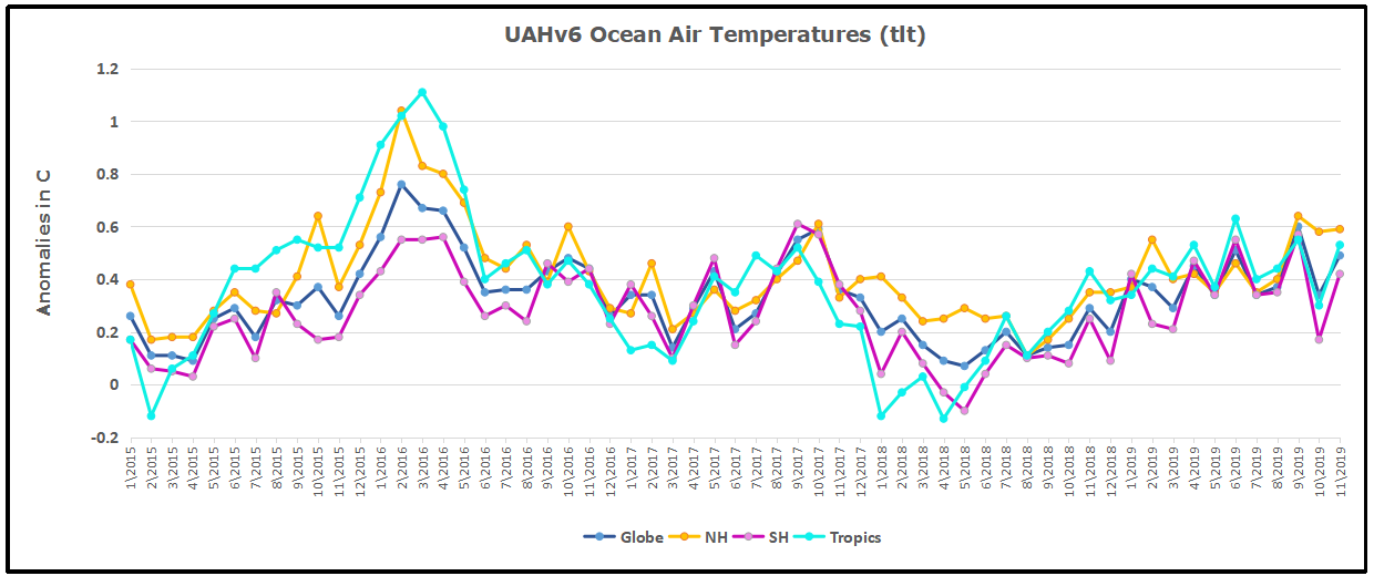 After a June rise in ocean air temps, all regions dropped back down to May levels in July and August. A spike occured in September, followed by plummenting October ocean air temps in the Tropics and SH. Now that drop has partly warmed back, leaving all regions in November slightly lower than September.
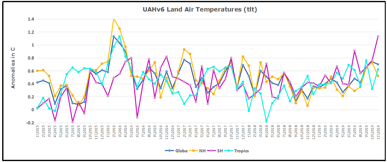 Here we have freash evidence of the greater volatility of the Land temperatures, along with an extraordinary departure by SH land. Despite the small amount of SH land, it spiked in July, then dropped in August so sharply along with the Tropics that it pulled the global average downward against slight warming in NH. Now again in November SH has jumped up beyond any month in this period. Despite this spike along with a rise in the Tropics, NH land temps dropped sharply. The larger NH land area pulled the Global average downward. The behavior of SH land temps is puzzling, to say the least.
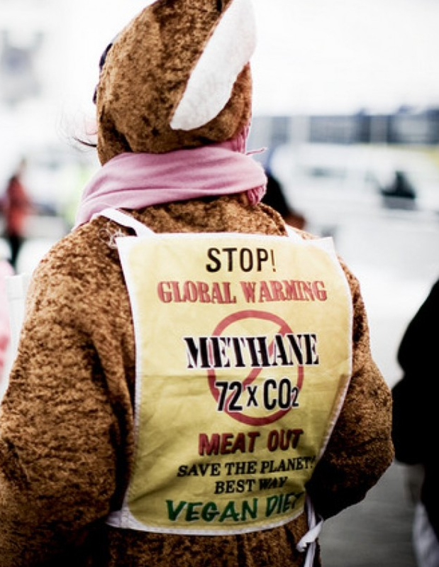
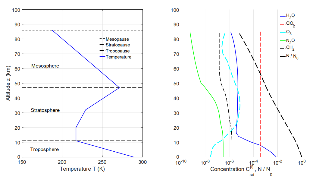


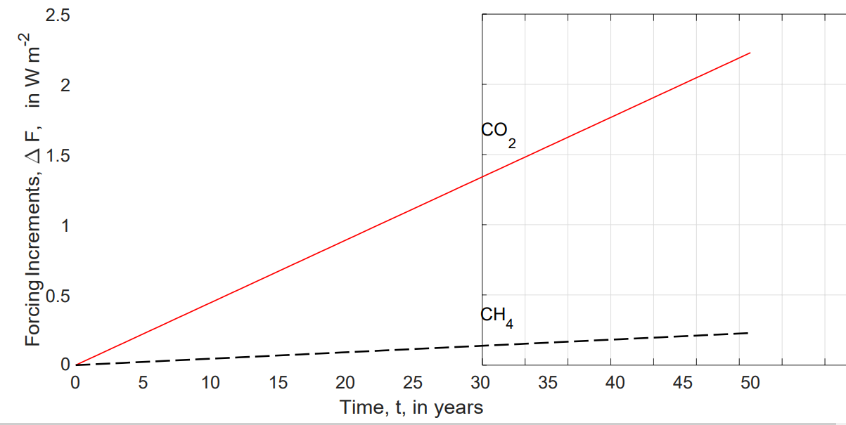


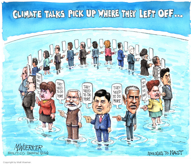


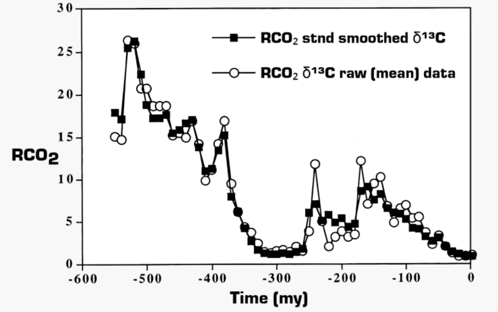

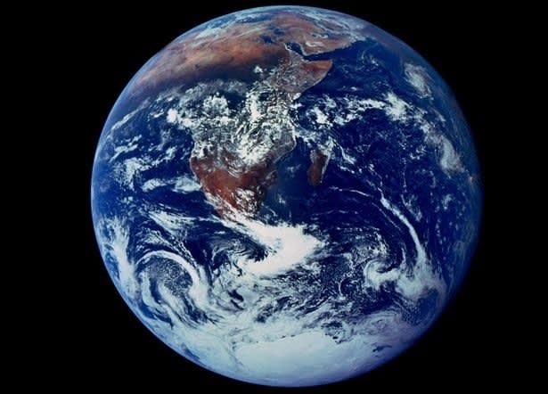
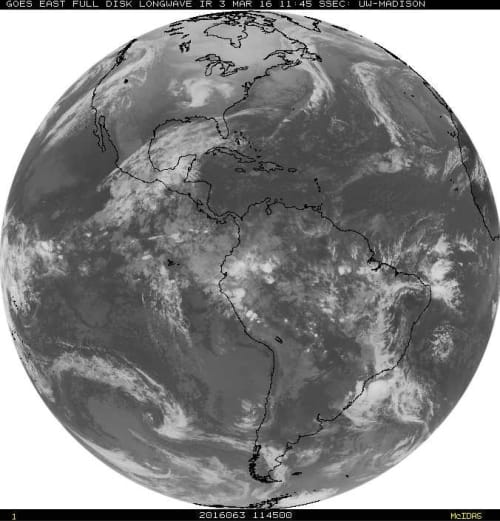
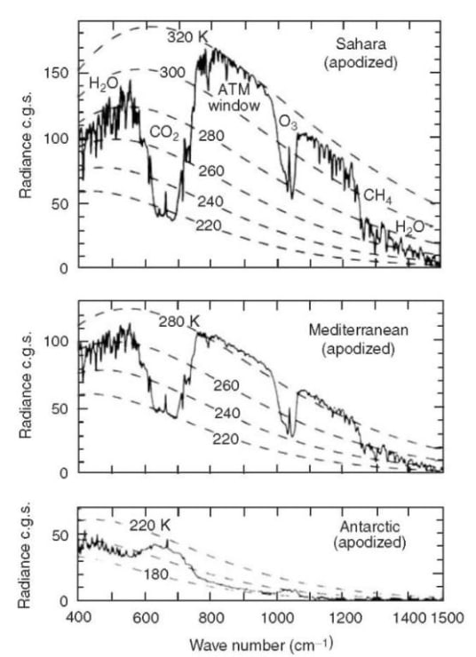
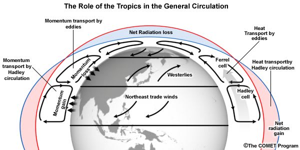


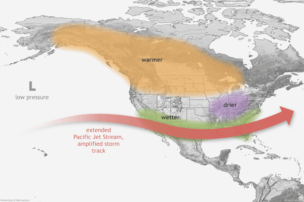
 Other scientists are more interested in the truth than in hype. An example is this AGU publication by D.A Smeed et al.

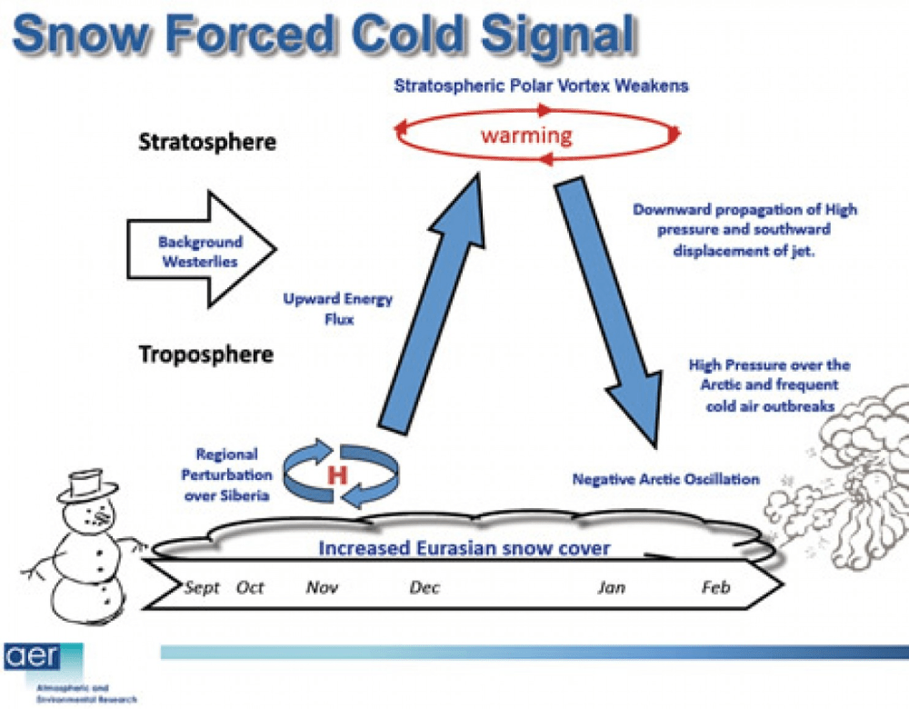


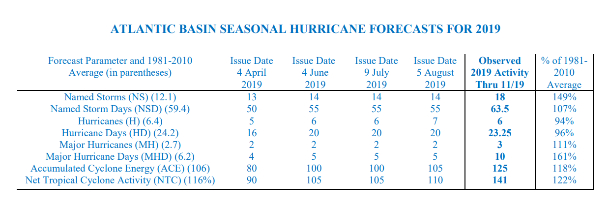


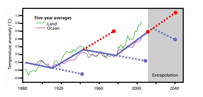
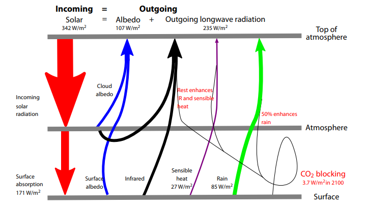
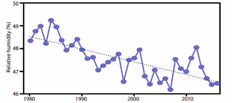
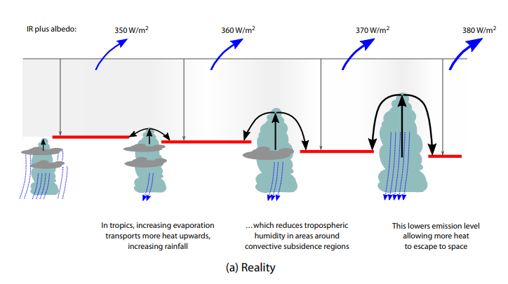
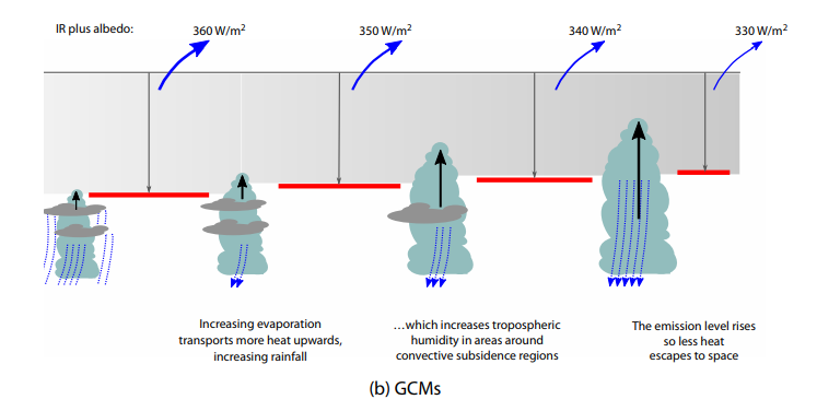
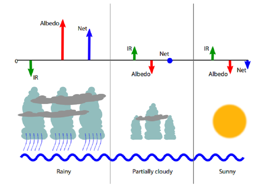
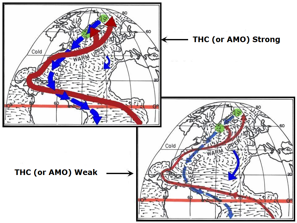
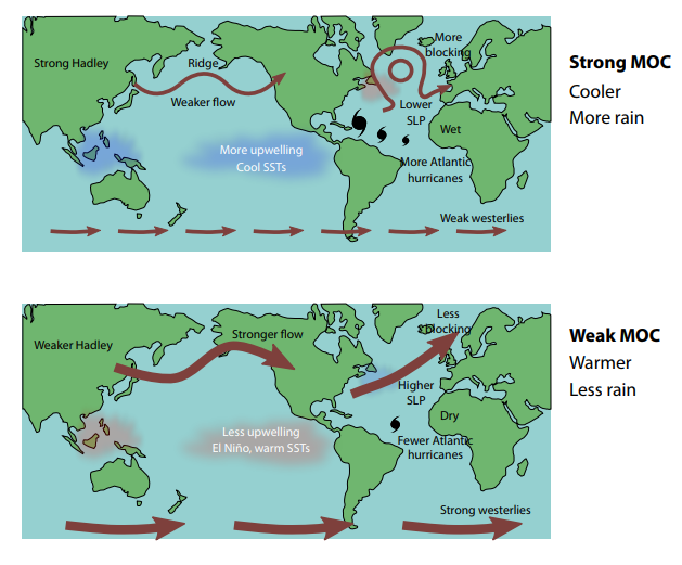
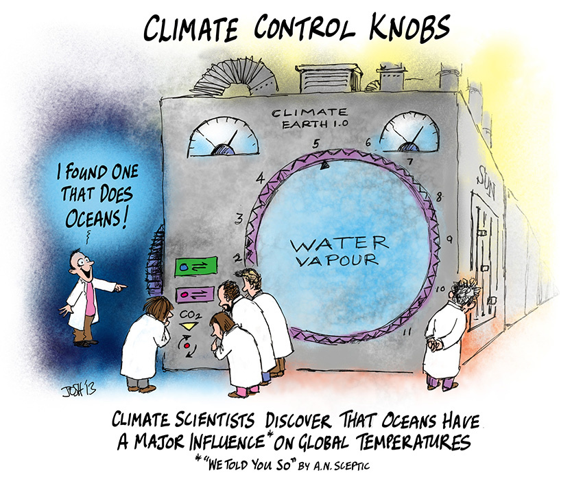


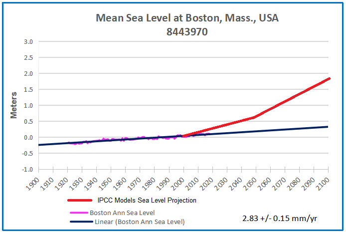
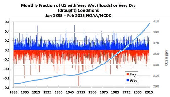
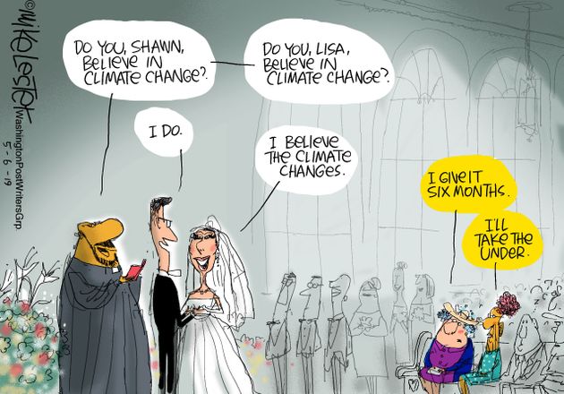


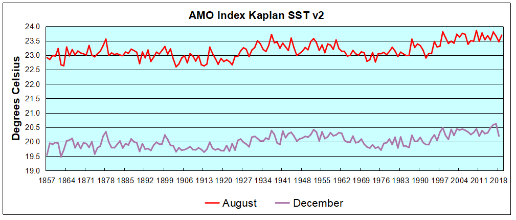


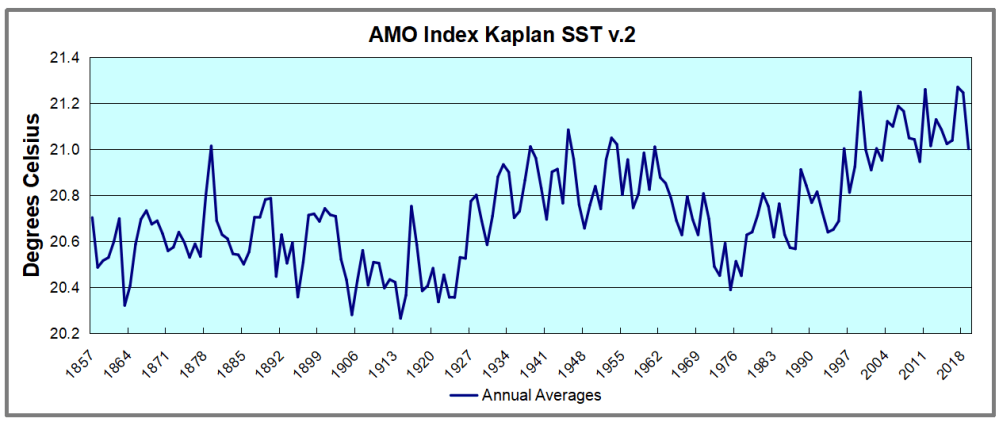
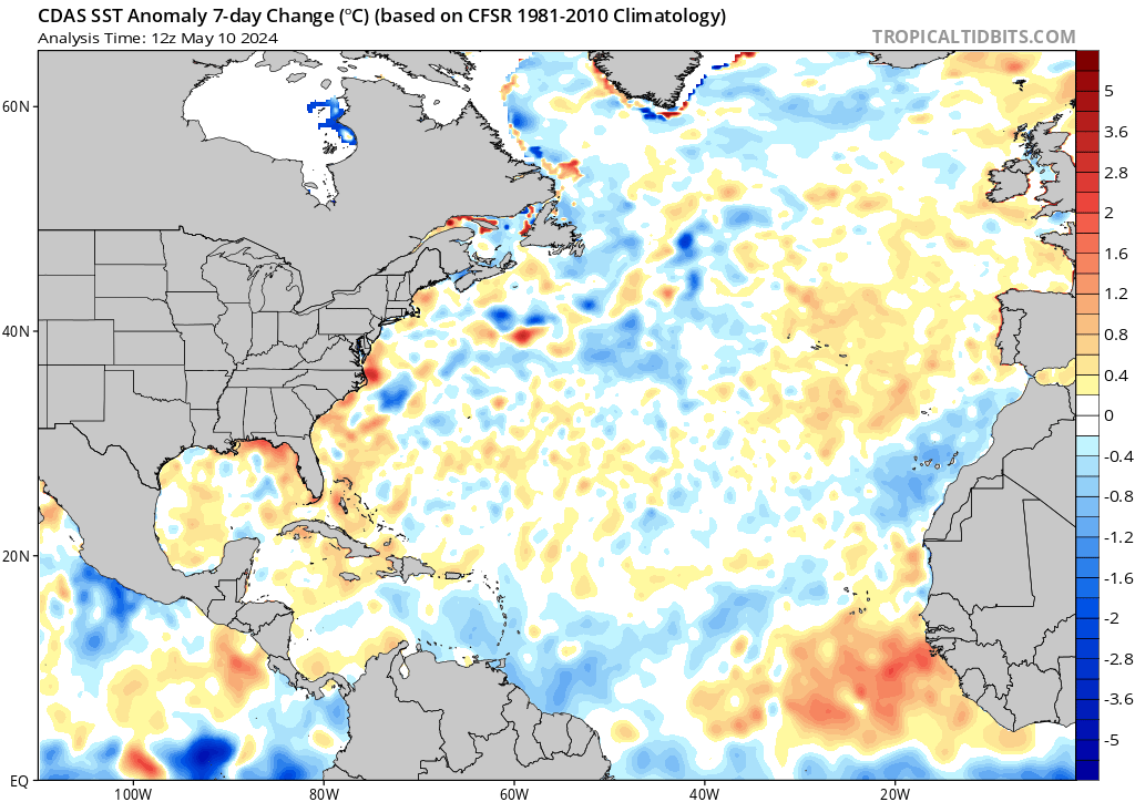
 The best context for understanding decadal temperature changes comes from the world’s sea surface temperatures (SST), for several reasons: