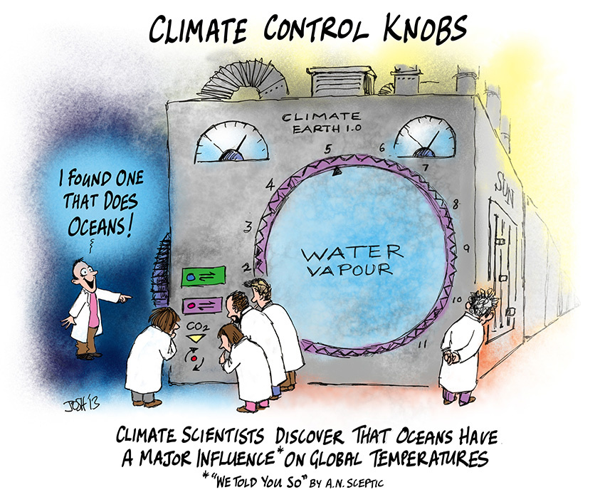
Bill Gray: H20 is Climate Control Knob, not CO2

William Mason Gray (1929-2016), pioneering hurricane scientist and forecaster and professor of atmospheric science at Colorado State University
Dr. William Gray made a compelling case for H2O as the climate thermostat, prior to his death in 2016. Thanks to GWPF for publishing posthumously Bill Gray’s understanding of global warming/climate change. The paper was compiled at his request, completed and now available as Flaws in applying greenhouse warming to Climate Variability This post provides some excerpts in italics with my bolds and some headers. Readers will learn much from the entire document (title above is link to pdf).
The Fundamental Correction
The critical argument that is made by many in the global climate modeling (GCM) community is that an increase in CO2 warming leads to an increase in atmospheric water vapor, resulting in more warming from the absorption of outgoing infrared radiation (IR) by the water vapor. Water vapor is the most potent greenhouse gas present in the atmosphere in large quantities. Its variability (i.e. global cloudiness) is not handled adequately in GCMs in my view. In contrast to the positive feedback between CO2 and water vapor predicted by the GCMs, it is my hypothesis that there is a negative feedback between CO2 warming and and water vapor. CO2 warming ultimately results in less water vapor (not more) in the upper troposphere. The GCMs therefore predict unrealistic warming of global temperature. I hypothesize that the Earth’s energy balance is regulated by precipitation (primarily via deep cumulonimbus (Cb) convection) and that this precipitation counteracts warming due to CO2.
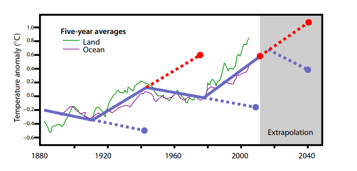
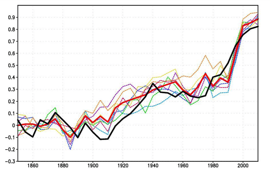
Figure 14: Global surface temperature change since 1880. The dotted blue and dotted red lines illustrate how much error one would have made by extrapolating a multi-decadal cooling or warming trend beyond a typical 25-35 year period. Note the recent 1975-2000 warming trend has not continued, and the global temperature remained relatively constant until 2014.
Projected Climate Changes from Rising CO2 Not Observed
Continuous measurements of atmospheric CO2, which were first made at Mauna Loa, Hawaii in 1958, show that atmospheric concentrations of CO2 have risen since that time. The warming influence of CO2 increases with the natural logarithm (ln) of the atmosphere’s CO2 concentration. With CO2 concentrations now exceeding 400 parts per million by volume (ppm), the Earth’s atmosphere is slightly more than halfway to containing double the 280 ppm CO2 amounts in 1860 (at the beginning of the Industrial Revolution).∗
We have not observed the global climate change we would have expected to take place, given this increase in CO2. Assuming that there has been at least an average of 1 W/m2 CO2 blockage of IR energy to space over the last 50 years and that this energy imbalance has been allowed to independently accumulate and cause climate change over this period with no compensating response, it would have had the potential to bring about changes in any one of the following global conditions:
- Warm the atmosphere by 180◦C if all CO2 energy gain was utilized for this purpose – actual warming over this period has been about 0.5◦C, or many hundreds of times less.
- Warm the top 100 meters of the globe’s oceans by over 5◦C – actual warming over this period has been about 0.5◦C, or 10 or more times less.
- Melt sufficient land-based snow and ice as to raise the global sea level by about 6.4 m. The actual rise has been about 8–9 cm, or 60–70 times less. The gradual rise of sea level has been only slightly greater over the last ~50 years (1965–2015) than it has been over the previous two ~50-year periods of 1915–1965 and 1865–1915, when atmospheric CO2 gain was much less.
- Increase global rainfall over the past ~50-year period by 60 cm.
Earth Climate System Compensates for CO2
If CO2 gain is the only influence on climate variability, large and important counterbalancing influences must have occurred over the last 50 years in order to negate most of the climate change expected from CO2’s energy addition. Similarly, this hypothesized CO2-induced energy gain of 1 W/m2 over 50 years must have stimulated a compensating response that acted to largely negate energy gains from the increase in CO2.
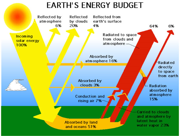
The continuous balancing of global average in-and-out net radiation flux is therefore much larger than the radiation flux from anthropogenic CO2. For example, 342 W/m2, the total energy budget, is almost 100 times larger than the amount of radiation blockage expected from a CO2 doubling over 150 years. If all other factors are held constant, a doubling of CO2 requires a warming of the globe of about 1◦C to enhance outward IR flux by 3.7 W/m2 and thus balance the blockage of IR flux to space.
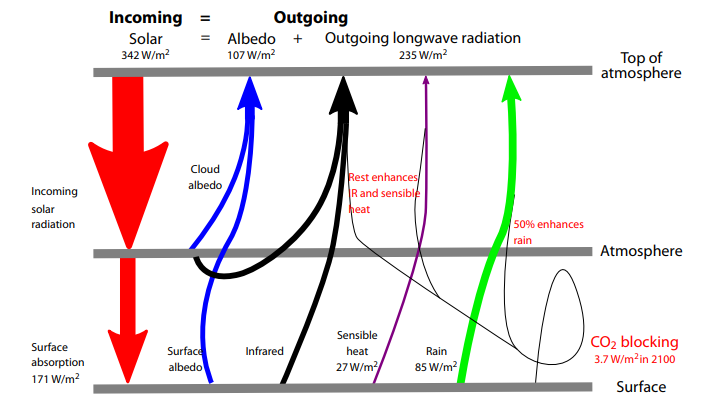
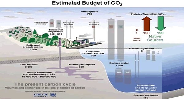
Figure 2: Vertical cross-section of the annual global energy budget. Determined from a combination of satellite-derived radiation measurements and reanalysis data over the period of 1984–2004.
This pure IR energy blocking by CO2 versus compensating temperature increase for radiation equilibrium is unrealistic for the long-term and slow CO2 increases that are occurring. Only half of the blockage of 3.7 W/m2 at the surface should be expected to go into an temperature increase. The other half (about 1.85 W/m2) of the blocked IR energy to space will be compensated by surface energy loss to support enhanced evaporation. This occurs in a similar way to how the Earth’s surface energy budget compensates for half its solar gain of 171 W/m2 by surface-to-air upward water vapor flux due to evaporation.
Assuming that the imposed extra CO2 doubling IR blockage of 3.7 W/m2 is taken up and balanced by the Earth’s surface in the same way as the solar absorption is taken up and balanced, we should expect a direct warming of only ~0.5◦C for a doubling of CO2. The 1◦C expected warming that is commonly accepted incorrectly assumes that all the absorbed IR goes to the balancing outward radiation with no energy going to evaporation.
Consensus Science Exaggerates Humidity and Temperature Effects
A major premise of the GCMs has been their application of the National Academy of Science (NAS) 1979 study3 – often referred to as the Charney Report – which hypothesized that a doubling of atmospheric CO2 would bring about a general warming of the globe’s mean temperature of 1.5–4.5◦C (or an average of ~3.0◦C). These large warming values were based on the report’s assumption that the relative humidity (RH) of the atmosphere remains quasiconstant as the globe’s temperature increases. This assumption was made without any type of cumulus convective cloud model and was based solely on the Clausius–Clapeyron (CC) equation and the assumption that the RH of the air will remain constant during any future CO2-induced temperature changes. If RH remains constant as atmospheric temperature increases, then the water vapor content in the atmosphere must rise exponentially.
With constant RH, the water vapor content of the atmosphere rises by about 50% if atmospheric temperature is increased by 5◦C. Upper tropospheric water vapor increases act to raise the atmosphere’s radiation emission level to a higher and thus colder level. This reduces the amount of outgoing IR energy which can escape to space by decreasing T^4.
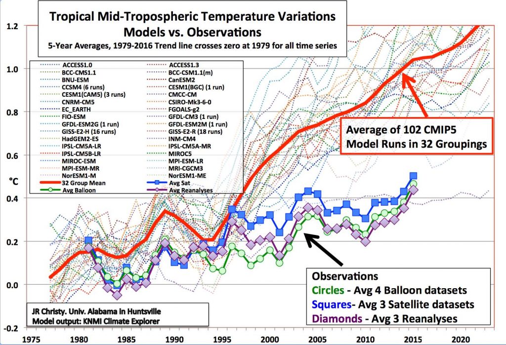
These model predictions of large upper-level tropospheric moisture increases have persisted in the current generation of GCM forecasts.§ These models significantly overestimate globally-averaged tropospheric and lower stratospheric (0–50,000 feet) temperature trends since 1979 (Figure 7).
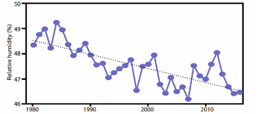
Figure 8: Decline in upper tropospheric RH. Annually-averaged 300 mb relative humidity for the tropics (30°S–30°N). From NASA-MERRA2 reanalysis for 1980–2016. Black dotted line is linear trend.
All of these early GCM simulations were destined to give unrealistically large upper-tropospheric water vapor increases for doubling of CO2 blockage of IR energy to space, and as a result large and unrealistic upper tropospheric temperature increases were predicted. In fact, if data from NASA-MERRA24 and NCEP/NCAR5 can be believed, upper tropospheric RH has actually been declining since 1980 as shown in Figure 8. The top part of Table 1 shows temperature and humidity differences between very wet and dry years in the tropics since 1948; in the wettest years, precipitation was 3.9% higher than in the driest ones. Clearly, when it rains more in the tropics, relative and specific humidity decrease. A similar decrease is seen when differencing 1995–2004 from 1985–1994, periods for which the equivalent precipitation difference is 2%. Such a decrease in RH would lead to a decrease in the height of the radiation emission level and an increase in IR to space.
The Earth’s natural thermostat – evaporation and precipitation
What has prevented this extra CO2-induced energy input of the last 50 years from being realized in more climate warming than has actually occurred? Why was there recently a pause in global warming, lasting for about 15 years? The compensating influence that prevents the predicted CO2-induced warming is enhanced global surface evaporation and increased precipitation.
Annual average global evaporational cooling is about 80 W/m2 or about 2.8 mm per day. A little more than 1% extra global average evaporation per year would amount to 1.3 cm per year or 65 cm of extra evaporation integrated over the last 50 years. This is the only way that such a CO2-induced , 1 W/m2 IR energy gain sustained over 50 years could occur without a significant alteration of globally-averaged surface temperature. This hypothesized increase in global surface evaporation as a response to CO2-forced energy gain should not be considered unusual. All geophysical systems attempt to adapt to imposed energy forcings by developing responses that counter the imposed action. In analysing the Earth’s radiation budget, it is incorrect to simply add or subtract energy sources or sinks to the global system and expect the resulting global temperatures to proportionally change. This is because the majority of CO2-induced energy gains will not go into warming the atmosphere. Various amounts of CO2-forced energy will go into ocean surface storage or into ocean energy gain for increased surface evaporation. Therefore a significant part of the CO2 buildup (~75%) will bring about the phase change of surface liquid water to atmospheric water vapour. The energy for this phase change must come from the surface water, with an expenditure of around 580 calories of energy for every gram of liquid that is converted into vapour. The surface water must thus undergo a cooling to accomplish this phase change.
Therefore, increases in anthropogenic CO2 have brought about a small (about 0.8%) speeding up of the globe’s hydrologic cycle, leading to more precipitation, and to relatively little global temperature increase. Therefore, greenhouse gases are indeed playing an important role in altering the globe’s climate, but they are doing so primarily by increasing the speed of the hydrologic cycle as opposed to increasing global temperature.
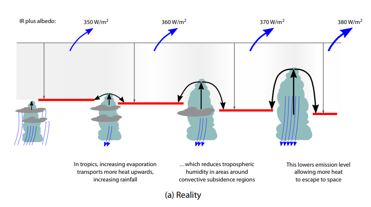
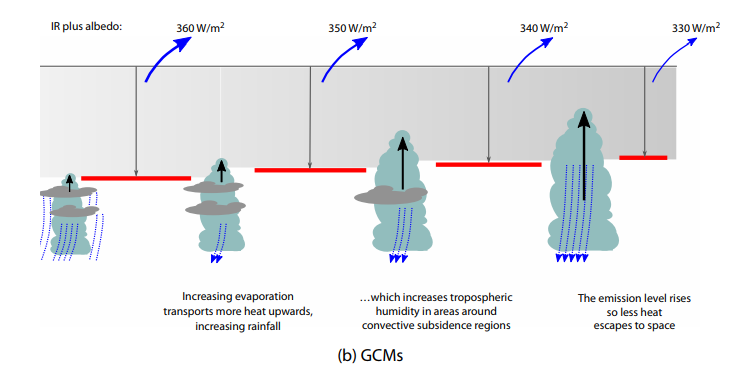 Figure 9: Two contrasting views of the effects of how the continuous intensification of deep
cumulus convection would act to alter radiation flux to space.
The top (bottom) diagram represents a net increase (decrease) in radiation to space
Tropical Clouds Energy Control Mechanism
It is my hypothesis that the increase in global precipitation primarily arises from an increase in deep tropical cumulonimbus (Cb) convection. The typical enhancement of rainfall and updraft motion in these areas together act to increase the return flow mass subsidence in the surrounding broader clear and partly cloudy regions. The upper diagram in Figure 9 illustrates the increasing extra mass flow return subsidence associated with increasing depth and intensity of cumulus convection. Rainfall increases typically cause an overall reduction of specific humidity (q) and relative humidity (RH) in the upper tropospheric levels of the broader scale surrounding convective subsidence regions. This leads to a net enhancement of radiation flux to space due to a lowering of the upper-level emission level. This viewpoint contrasts with the position in GCMs, which suggest that an increase in deep convection will increase upper-level water vapour.
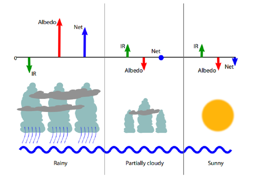
Figure 10: Conceptual model of typical variations of IR, albedo and net (IR + albedo) associated with three different areas of rain and cloud for periods of increased precipitation.
The albedo enhancement over the cloud–rain areas tends to increase the net (IR + albedo) radiation energy to space more than the weak suppression of (IR + albedo) in the clear areas. Near-neutral conditions prevail in the partly cloudy areas. The bottom diagram of Figure 9 illustrates how, in GCMs, Cb convection erroneously increases upper tropospheric moisture. Based on reanalysis data (Table 1, Figure 8) this is not observed in the real atmosphere.
Ocean Overturning Circulation Drives Warming Last Century
A slowing down of the global ocean’s MOC is the likely cause of most of the global warming that has been observed since the latter part of the 19th century.15 I hypothesize that shorter multi-decadal changes in the MOC16 are responsible for the more recent global warming periods between 1910–1940 and 1975–1998 and the global warming hiatus periods between 1945–1975 and 2000–2013.
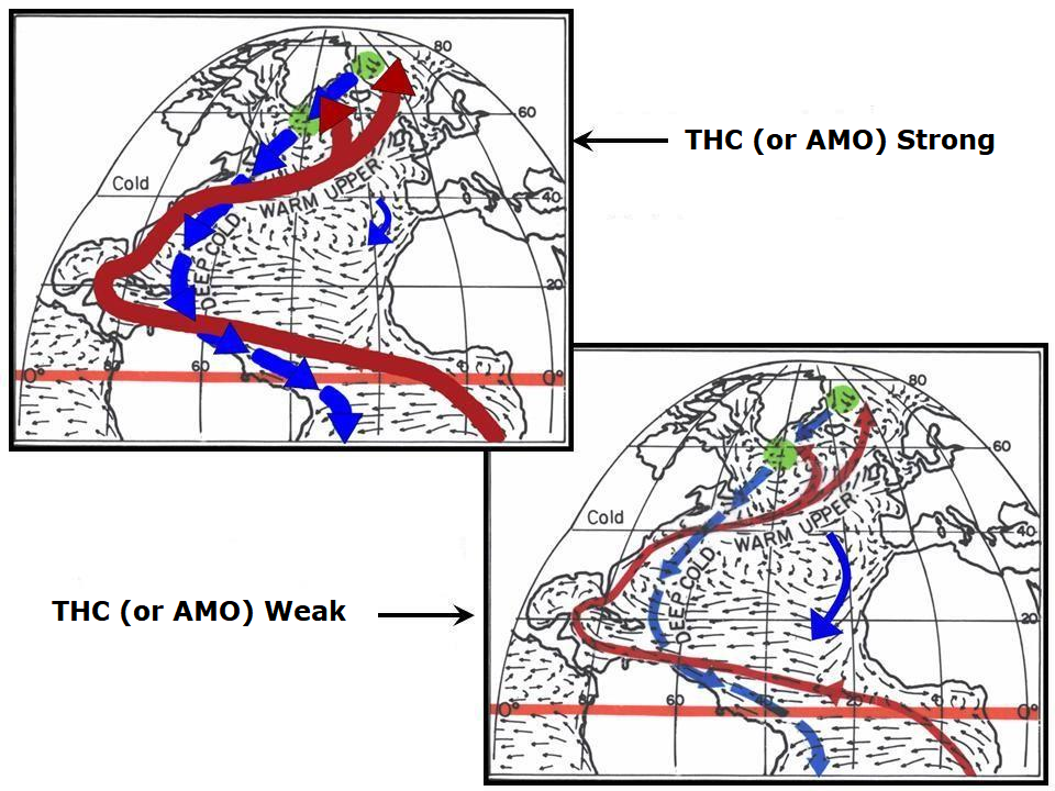
Figure 12: The effect of strong and weak Atlantic THC. Idealized portrayal of the primary Atlantic Ocean upper ocean currents during strong and weak phases of the thermohaline circulation (THC)
Figure 13 shows the circulation features that typically accompany periods when the MOC is stronger than normal and when it is weaker than normal. In general, a strong MOC is associated with a warmer-than-normal North Atlantic, increased Atlantic hurricane activity, increased blocking action in both the North Atlantic and North Pacific and weaker westerlies in the mid-latitude Southern Hemisphere. There is more upwelling of cold water in the South Pacific and Indian Oceans, and an increase in global rainfall of a few percent occurs. This causes the global surface temperatures to cool. The opposite occurs when the MOC is weaker than normal.
The average strength of the MOC over the last 150 years has likely been below the multimillennium average, and that is the primary reason we have seen this long-term global warming since the late 19th century. The globe appears to be rebounding from the conditions of the Little Ice Age to conditions that were typical of the earlier ‘Medieval’ and ‘Roman’ warm periods.
Summary and Conclusions
The Earth is covered with 71% liquid water. Over the ocean surface, sub-saturated winds blow, forcing continuous surface evaporation. Observations and energy budget analyses indicate that the surface of the globe is losing about 80 W/m2 of energy from the global surface evaporation process. This evaporation energy loss is needed as part of the process of balancing the surface’s absorption of large amounts of incoming solar energy. Variations in the strength of the globe’s hydrologic cycle are the way that the global climate is regulated. The stronger the hydrologic cycle, the more surface evaporation cooling occurs, and greater the globe’s IR flux to space. The globe’s surface cools when the hydrologic cycle is stronger than average and warms when the hydrologic cycle is weaker than normal. The strength of the hydrologic cycle is thus the primary regulator of the globe’s surface temperature. Variations in global precipitation are linked to long-term changes in the MOC (or THC).
I have proposed that any additional warming from an increase in CO2 added to the atmosphere is offset by an increase in surface evaporation and increased precipitation (an increase in the water cycle). My prediction seems to be supported by evidence of upper tropospheric drying since 1979 and the increase in global precipitation seen in reanalysis data. I have shown that the additional heating that may be caused by an increase in CO2 results in a drying, not a moistening, of the upper troposphere, resulting in an increase of outgoing radiation to space, not a decrease as proposed by the most recent application of the greenhouse theory.
Deficiencies in the ability of GCMs to adequately represent variations in global cloudiness, the water cycle, the carbon cycle, long-term changes in deep-ocean circulation, and other important mechanisms that control the climate reduce our confidence in the ability of these models to adequately forecast future global temperatures. It seems that the models do not correctly handle what happens to the added energy from CO2 IR blocking.
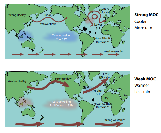
Figure 13: Effect of changes in MOC: top, strong MOC; bottom weak MOC. SLP: sea level pressure; SST, sea surface temperature.
Solar variations, sunspots, volcanic eruptions and cosmic ray changes are energy-wise too small to play a significant role in the large energy changes that occur during important multi-decadal and multi-century temperature changes. It is the Earth’s internal fluctuations that are the most important cause of climate and temperature change. These internal fluctuations are driven primarily by deep multi-decadal and multi-century ocean circulation changes, of which naturally varying upper-ocean salinity content is hypothesized to be the primary driving mechanism. Salinity controls ocean density at cold temperatures and at high latitudes where the potential deep-water formation sites of the THC and SAS are located. North Atlantic upper ocean salinity changes are brought about by both multi-decadal and multi-century induced North Atlantic salinity variability.
Footnote:
The main point from Bill Gray was nicely summarized in a previous post Earth Climate Layers
The most fundamental of the many fatal mathematical flaws in the IPCC related modelling of atmospheric energy dynamics is to start with the impact of CO2 and assume water vapour as a dependent ‘forcing’. This has the tail trying to wag the dog. The impact of CO2 should be treated as a perturbation of the water cycle. When this is done, its effect is negligible. — Dr. Dai Davies


 The best context for understanding decadal temperature changes comes from the world’s sea surface temperatures (SST), for several reasons:
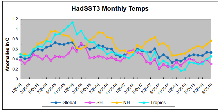


/cdn.vox-cdn.com/uploads/chorus_image/image/56293121/total_solar_eclipse.0.jpg)


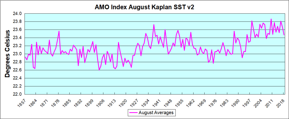
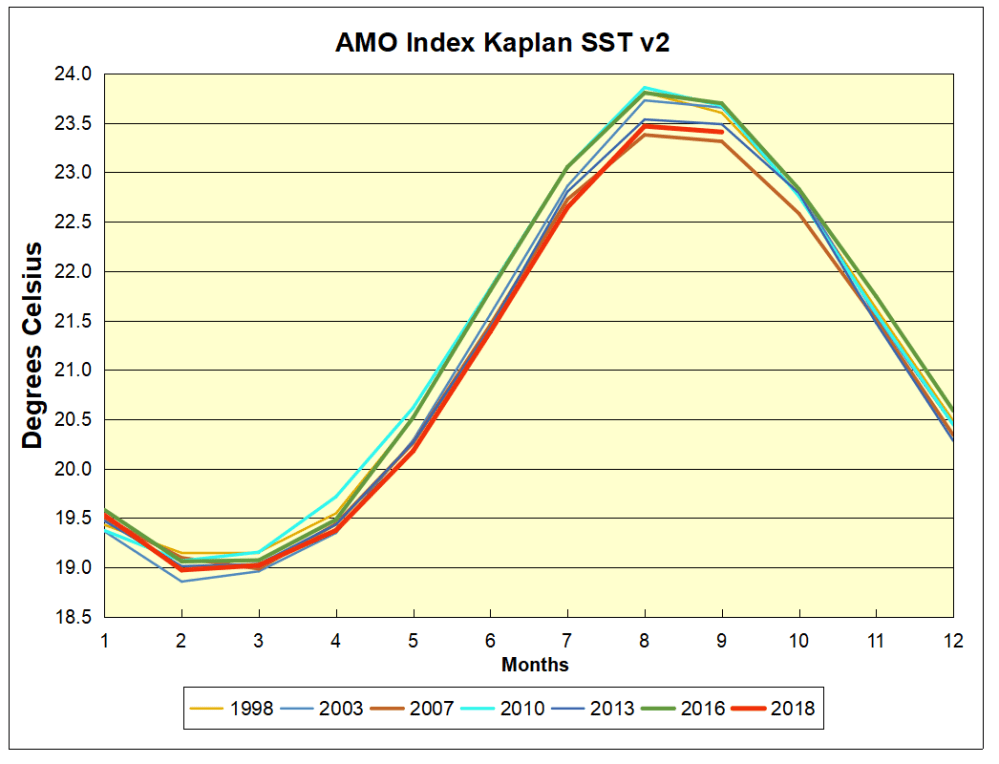
 The AMO Index is from from Kaplan SST v2, the unaltered and untrended dataset. By definition, the data are monthly average SSTs interpolated to a 5×5 grid over the North Atlantic basically 0 to 70N. The graph shows warming began after 1992 up to 1998, with a series of matching years since. September is the second hottest month in the dataset, and note the considerable drop from 2017 to August 2018. Because McCarthy refers to hints of cooling to come in the N. Atlantic, let’s take a closer look at some AMO years in the last 2 decades.


 The anomalies over the entire ocean dropped to the same value, 0.12C in August (Tropics were 0.13C). Warming in previous months was erased, and September added very little warming back.


