H20 the Gorilla Climate Molecule

In climate discussions, someone is bound to say: Climate is a lot more than temperatures. And of course, they are right. So let’s consider the other major determinant of climate, precipitation.
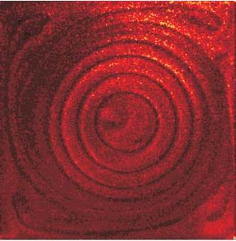
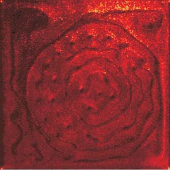
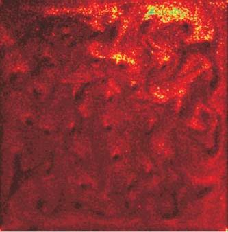
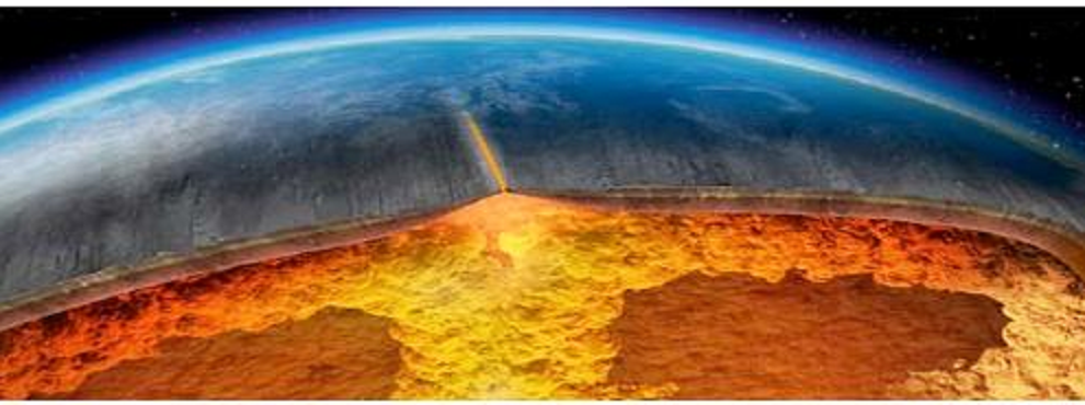
The chart above is actually a screen capture of real-time measurements of precipitable water in the atmosphere. The 24-hour animation can be accessed at MIMIC-TPW ver.2 . H/T Ireneusz Palmowski, who commented: “I do not understand why scientists deal with anthropogenic CO2, although the entire convection in the troposphere is driven by water vapor (and ozone in high latitudes).”
These images show that H2O is driving the heat engine through its phase changes (liquid to vapor to liquid (and sometimes ice crystals as well). And as far as radiative heat transfer is concerned, 95% of it is done by water molecules. Below is an essay going into the dynamics of precipitation, its variability over the earth’s surface, and its role in determining regional, and even microclimates. The post was originally titled “Here Comes the Rain Again, inspired by the Eurythmics classic song
The global story on rain is straightforward:
“Precipitation is a major component of the water cycle, and is responsible for depositing the fresh water on the planet. Approximately 505,000 cubic kilometres (121,000 cu mi) of water falls as precipitation each year; 398,000 cubic kilometres (95,000 cu mi) of it over the oceans. Given the Earth’s surface area, that means the globally averaged annual precipitation is 990 millimetres (39 in). Climate classification systems such as the Köppen climate classification system use average annual rainfall to help differentiate between differing climate regimes.
http://en.wikipedia.org/wiki/Precipitation_(meteorology)
Globally, average precipitation can vary from +/-5% yearly, but there is no particular trend in the history of observations. But rain is one of those things where averages don’t tell you much. For starters, look at where it’s coming down:

So about 1 meter a year is the nominal average of all rain over all surfaces. Some places get up to 10 meters of rain (about 400 inches ) and others get near none. 47% of the earth is considered dryland, defined as anyplace where the rate of evaporation/transpiration exceeds the rate of precipitation. A desert is defined as a dryland with less than 25 cm of precipitation. In the image above, polar deserts are remarkably defined. It just does not have much hope of precipitation as there is little heat to move the water. More heat in, more water movement. Less heat in, less water movement.
Then there’s the seasonal patterns. The band of maximum rains moves with the sun: More north in June, more south in December. More sun, more heating, more rain. Movement in sync with the sun, little time delay. Equatorial max solar heat has max rains. Polar zones minimal heating, minimal precipitation. It’s a very tightly coupled system with low time lags.
The other obvious thing is how central land areas get dry desert conditions if they are not in the equatorial band nor near a warm water current. Brazil, in particular, benefits from warm coastal waters and near equatorial rains. The Gulf Stream rescues Europe from a much drier climate, but I fear the Gulf Stream shifting of zones also puts parts of Saharan Africa out of the equatorial wet. (In some times during history it DOES get a load of water, though…)
From E.M. Smith
https://chiefio.wordpress.com/2011/11/01/what-does-precipitation-say-about-heat-flow/
How do Oceans Make Rain
Here I am taking direction from A. M Makarieva and her colleagues. She explains:
“Water vapor originating by evaporation sustained by solar radiation represents a source of ordered potential energy that is available for generation of atmospheric circulation, including the biotic pump. We will further consider details of this process.

As we can see, early in its life the cloud expands in all directions, meanwhile the air continues to converge towards the (growing) condensation area. This process is at the core of condensation-induced dynamics: as condensation occurs and local pressure drops, this initiates convergence and ascent. They, in their turn, feedback positively on condensation intensity, such that the air pressure lowers further, convergence becomes more extensive and so on — as long as there is enough water vapor around to feed the process.
And where does the water vapor come from? Ocean evaporation, 87%, Plant transpiration 10% , Other evaporation, lakes, rivers, etc. 3%.
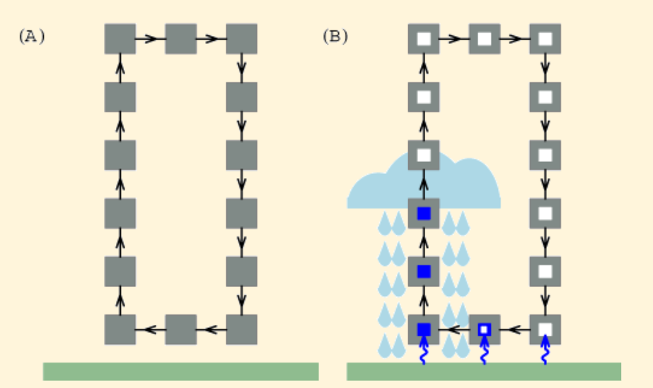
Air circulation without condensation (A) and with condensation (B). Gray squares are the air volumes, which in case (B) contain water vapor shown by small blue squares inside gray ones. White squares indicate those air volumes that have lost their water vapor owing to condensation. Blue arrows at the Earth’s surface represent evaporation that replenishes the store of water vapor in the circulating air.
On Fig. B we can see a circulation accompanied by water vapor condensation (water vapor is shown by blue squares). At a certain height water vapor condenses leaving the gaseous phase, while the remaining air continues to circulate deprived of water vapor (this depletion is shown by empty white squares): it first rises and then descends. As one can see, in such a circulation total mass of the rising air would be larger than total mass of the descending air (cf. an escalator transporting people up). The motor driving such a circulation would not only have to compensate the friction losses, but also have to work against gravity that is acting on the ascending air.
One can see from Fig. B that the difference between the cumulative masses of the ascending and descending air parcels grows with increasing height where condensation occurs. This difference also grows with increasing amount of water vapor in the air (i.e. with increasing size of the blue squares). The dynamic power of condensation, on the other hand, is also proportional to the amount of water vapor, but it is practically independent of condensation height.
Condensation height (a proxy for precipitation pathlength) grows with increasing temperature of the Earth’s surface. It is shown in the paper that power losses associated with precipitation of condensate particles become equal to the total dynamic power of condensation at surface temperatures around 50 degrees Celsius. Since the observed power of condensation-driven winds is equal to the total dynamic power of condensation (the “motor”) minus the power spent on compensating precipitation, at such temperatures the observed circulation power becomes zero and the circulation must stop. For commonly observed values of surface temperature these losses do no exceed 40% of condensation power and cannot arrest the condensation-induced circulation. Over 60% of condensation power is spent on friction at the Earth’s surface.
Why Some Places Get More Rain Than Others

This figure shows the “tug-of-war” between the forest and the ocean for the right to become a predominant condensation zone. In Fig. a: on average the Amazon and Congo forests win this war: annual precipitation over forests is two to three times larger than the precipitation over the Atlantic Ocean at the same latitude. Note the logarithmic scale on the vertical axis: “1” means that the land/ocean precipitation ratio is equal to e = 2.718, “2” means it is equal to e2 ≈ 7.4; “0” means that this ratio is unity (equal precipitation on land and the ocean); “-1” means this ratio is 1/e ≈ 0.4; and so on.
In Fig. b: the Eurasian biotic pump. In winter the forest sleeps, so the ocean wins, and all moisture remains over the ocean and precipitates there. In summer, when trees are active, moisture is taken from the ocean and distributed regularly over seven thousand kilometers. The forest wins! (compare the red and black lines) As a result, precipitation over the ocean in summer is lower than it is in winter, despite the temperature in summer is higher.
Finally, in panel (c): an unforested Australia. One can often hear that Australia is so dry because it is situated in the descending branch of the Hadley cell. But this figure shows that such an interpretation does not hold. Both in wet and dry seasons precipitation over Australia is four to six times lower than over the ocean. There is no biotic pump there. Being unforested, oceanic moisture cannot penetrate to the Australian continent irrespective of how much moisture there is over the ocean; during the wet season it precipitates in the coastal zones causing floods. Gradually restoring natural forests in Australia from coast to interior will recover the hydrological cycle on the continent.
http://www.bioticregulation.ru/pump/pump9.php

The Biotic Pump A. M Makarieva et al
Water cycle on land owes itself to the atmospheric moisture transport from the ocean. Properties of the aerial rivers that ensure the “run-in” of water vapor inland to compensate for the gravitational “run-off” of liquid water from land to the ocean are of direct relevance for the regional water availability. The biotic pump concept clarifies why the moist aerial rivers flow readily from ocean to land when the latter gives home to a large forest — and why they are reluctant to do so when the forest is absent.
While it is increasingly common to blame global change for any regional water cycle disruption, the biotic pump evidence suggests that the burden of responsibility rather rests with the regional land use practices. On large areas on both sides of the Atlantic Ocean, temperate and boreal forests are intensely harvested for timber and biofuel. These forests are artificially maintained in the early successional stages and are never allowed to recover to the natural climax state. The water regulation potential of such forests is low, while their susceptibility to fires and pests is high.
https://2s3c.wordpress.com/2012/04/22/taac/
Conclusion
So the oceans make rain, and together with the forests the land receives its necessary fresh water. There is a threat from human activity, but it has nothing to do with CO2. Land use practices leading to deforestation have the potential to disrupt this process. Without trees attracting the moist air from the ocean there is desert.
Ironically, modern societies burn fossil fuels instead of burning the forests as in the past.
For more on climate science related to H2O, see Bill Gray: H20 is Climate Control Knob, not CO2