A post last month noted that Arctic ice extent in February unusually exceeded 15M km2 (15 Wadhams). This was despite slower than usual recovery of ice in Sea of Okhotsk. That early 2022 peak ice extent has passed and will now stand as 2022 annual maximum. One wonders why the large ice deficit in that basin. The graph below shows the anomaly.
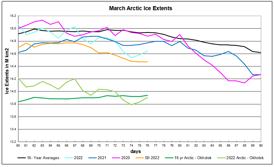
The 2022 cyan line started March above 15M km2, then declined to day 76 (March 17), ~300k km2 lower than the 16 yr. average. The dark green line shows Arctic ice extent average after Okhotsk is excluded, while the light green is 2022 Arctic extent without Okhotsk. The table below shows that Okhotsk deficit to average on day 76 is 260k km2, almost the entire Arctic deficit.
| Region | 2022076 | Day 76 Average | 2022-Ave. | 2021076 | 2022-2021 |
| (0) Northern_Hemisphere | 14641084 | 14935497 | -294413 | 14769906 | -128822 |
| (1) Beaufort_Sea | 1070776 | 1070247 | 529 | 1070689 | 87 |
| (2) Chukchi_Sea | 966006 | 965877 | 129 | 966006 | 0 |
| (3) East_Siberian_Sea | 1087137 | 1087107 | 30 | 1087120 | 17 |
| (4) Laptev_Sea | 897845 | 897837 | 8 | 897827 | 18 |
| (5) Kara_Sea | 905846 | 923576 | -17730 | 935006 | -29160 |
| (6) Barents_Sea | 554036 | 648194 | -94158 | 849221 | -295185 |
| (7) Greenland_Sea | 572046 | 618979 | -46934 | 601423 | -29377 |
| (8) Baffin_Bay_Gulf_of_St._Lawrence | 1784542 | 1534462 | 250080 | 1288815 | 495727 |
| (9) Canadian_Archipelago | 854685 | 853020 | 1665 | 854597 | 88 |
| (10) Hudson_Bay | 1260691 | 1258149 | 2542 | 1260471 | 220 |
| (11) Central_Arctic | 3153037 | 3223013 | -69976 | 3222708 | -69671 |
| (12) Bering_Sea | 729277 | 755358 | -26081 | 547775 | 181502 |
| (13) Baltic_Sea | 59785 | 81419 | -21634 | 62626 | -2841 |
| (14) Sea_of_Okhotsk | 739183 | 998164 | -258981 | 1117615 | -378432 |
Most places are close to average, with a large surplus in Baffin Bay offsetting small deficits elsewhere. The exception is Okhotsk making up most of the total deficit to average, and even a larger deficit to last year
IOW, had Okhotsk extent been average on day 60 (1.08M km2) instead of 852k km2, the surplus would have been even higher. So why was ice missing in Okhotsk this year?
Firstly, the animation above shows that Okhotsk (and also Bering) sea ice is quite variable year over year. The MASIE record for day 60 shows Okhotsk at 880k km2 in 2006, up to 1230k km2 in 2012, down to 770k km2 in 2015, up to 1080k km2 in 2018, down to 850k km2 in 2022. Notice Okhotsk 2022 is quite similar to 2015, while Bering is about average this year. What causes these fluctuations on annual, decadal and longer time scales?
The answer illustrates the complexity of natural factors interacting to produce climatic patterns we observe and measure. In Okhotsk in particular, and in the Arctic generally, changes in ice extents are a function of the 3 Ws: Water, Wind and Weather. More specifically, water changes in temperature (SST) and salinity (SSS); wind changes with changes in sea level pressures (SLP); and stormy weather varies between cyclonic and anticyclonic regimes. Below is discussion of these natural mechanisms.
Background on Okhotsk Sea
NASA describes Okhotsk as a Sea and Ice Factory. Excerpts in italics with my bolds.
The Sea of Okhotsk is what oceanographers call a marginal sea: a region of a larger ocean basin that is partly enclosed by islands and peninsulas hugging a continental coast. With the Kamchatka Peninsula, the Kuril Islands, and Sakhalin Island partly sheltering the sea from the Pacific Ocean, and with prevailing, frigid northwesterly winds blowing out from Siberia, the sea is a winter ice factory and a year-round cloud factory.
The region is the lowest latitude (45 degrees at the southern end) where sea ice regularly forms. Ice cover varies from 50 to 90 percent each winter depending on the weather. Ice often persists for nearly six months, typically from October to March. Aside from the cold winds from the Russian interior, the prodigious flow of fresh water from the Amur River freshens the sea, making the surface less saline and more likely to freeze than other seas and bays.
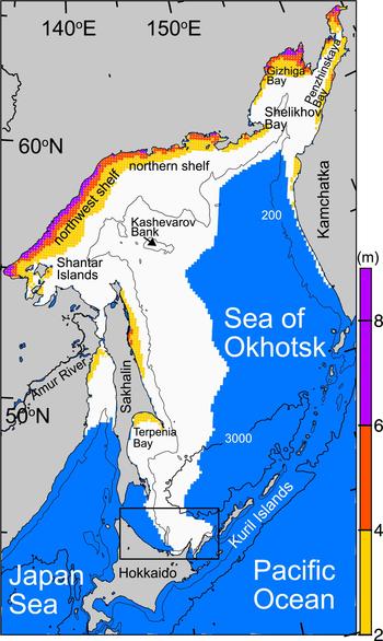
Map of the Sea of Okhotsk with bottom topography. The 200- and 3000-m isobars are indicated by thin and thick solid lines, respectively. A box denotes the enlarged portion in Figure 5. White shading indicates sea-ice area (ice concentration ⩾30%) in February averaged for 2003–11; blue shading indicates open ocean area. Ice concentration from AMSR-E is used. Color shadings indicate cumulative ice production in coastal polynyas during winter (December–March) averaged from the 2002/03 to 2009/10 seasons (modified from Nihashi and others, 2012, 2017). The amount is indicated by the bar scale. Source: Cambridge Core
Basics of Weather and Ice Dynamics
Wind directions are named by which point on the compass the prevailing wind hits you in the face. Thus, a southerly wind comes from the south toward the north, typically bringing warmer air north, and displacing colder northern air.
Winds arise from differences in surface pressures. Above every square inch on the surface of the Earth is 14.7 pounds of air. That means air exerts 14.7 pounds per square inch (psi) of pressure at Earth’s surface. High in the atmosphere, air pressure decreases.
Pressure varies from day to day at the Earth’s surface – the bottom of the atmosphere. This is, in part, because the Earth is not equally heated by the Sun. Areas where the air is warmed often have lower pressure because the warm air rises. These areas are called low pressure systems. Places where the air pressure is high, are called high pressure systems.
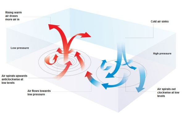
A low pressure system has lower pressure at its center than the areas around it. Winds blow towards the low pressure, and the air rises in the atmosphere where they meet. As the air rises, the water vapor within it condenses, forming clouds and often precipitation. Because of Earth’s spin and the Coriolis effect, winds of a low pressure system swirl counterclockwise north of the equator and clockwise south of the equator. This is called cyclonic flow. On weather maps, a low pressure system is labeled with red L.
A high pressure system has higher pressure at its center than the areas around it. Winds blow away from high pressure. Swirling in the opposite direction from a low pressure system, the winds of a high pressure system rotate clockwise north of the equator and counterclockwise south of the equator. This is called anticyclonic flow. Air from higher in the atmosphere sinks down to fill the space left as air is blown outward. On a weather map, you may notice a blue H, denoting the location of a high pressure system.

High and low pressure indicated by lines of equal pressure called isobars.
When the suns shines on land the air is warmed and rises. And because the earth is rotating, an upward spiral forms. Additionally, over wetlands and the oceans there is evaporation, which also rises, H2O being lighter than N2 or O2. When the water is warmer, the rising air intensifies and resulting in a lower pressure than surrounding areas. Arctic cyclones disrupt drift ice, creating more open water, and impede freezing. Arctic anticyclones (HP cells) facilitate cooling and freezing.
The vertical direction of wind motion is typically very small (except in thunderstorm updrafts) compared to the horizontal component, but is very important for determining the day to day weather. Rising air will cool, often to saturation, and can lead to clouds and precipitation. Sinking air warms causing evaporation of clouds and thus fair weather.
The closer the isobars are drawn together the quicker the air pressure changes. This change in air pressure is called the “pressure gradient”. Pressure gradient is just the difference in pressure between high- and low-pressure areas.
The Okhotsk Sea Ice Connection
Toyoda et al. (2022) explain in their paper Sea ice variability along the Okhotsk coast of Hokkaido based on long-term JMA meteorological observatory data. Excerpts in italics with my bolds.
Abstract
Long-term sea ice observation data at the Japan Meteorological Agency observatories along the
Okhotsk coast of Hokkaido were analyzed. The observations at the Abashiri Local Meteorological
Observatory largely explained the variations at other sites along much of the Okhotsk coast on a time scale longer than a few days. Interannually, variations of the maximum sea ice areas in the whole and southern Sea of Okhotsk were largely reflected in the yearly accumulated sea ice concentration (SIC) and sea ice duration variations at the observatories.
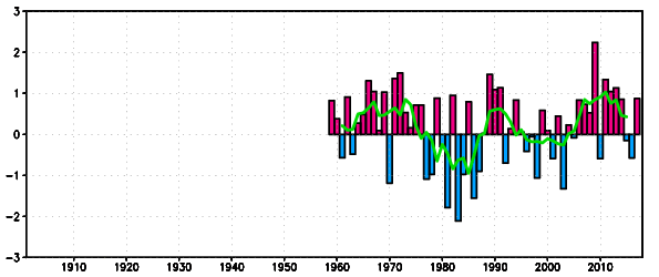
NPI time series The bars represent five-month mean ( November – March ) NPI values. The green line represents five-year running means of five-month mean NPI values. Positive (negative) NPI values indicate that the Aleutian Low is weaker (stronger) than its normal. For comparison with the PDO index, the period of the graph is adjusted to that of the PDO index.
A comparison with several indices for the North Pacific climate variability suggested that the North Pacific Index (NPI) is a robust indicator of the recent (after the 1980s) sea ice variations in the Sea of Okhotsk on a decadal time scale. Specifically:
♦ variations in the first sea ice appearance date at the observatories resulted from variations in the Aleutian Low with meridional wind anomalies over the Sea of Okhotsk and the air temperature around Japan in January;
♦ variations in the final disappearance date resulted from the Aleutian Low variations, and,
♦ the resulting sea ice cover variations in the Sea of Okhotsk except for the Siberian coast affected the air temperatures in April. These factors influenced the sea ice duration.
A strong linkage was found between variations in the local sea ice (along the Hokkaido coast) and large-scale fields, which will help improve our understanding of the sea ice extent and retreat variability over the Sea of Okhotsk and its linkage to the North Pacific climate variability.
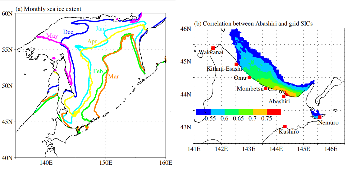
Fig. 1 (a) Monthly sea ice extent (contours of grid SIC = 0.3) averaged over 1977–2019. (b) Locations of JMA observatories and distribution of dailybasis correlation coefficients between the Abashiri and grid SICs. (N = 700–800 approximately).
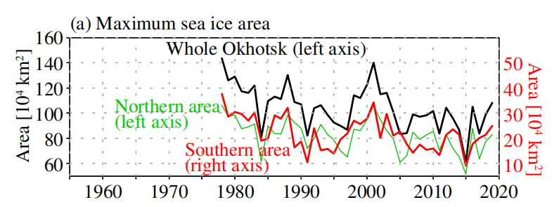
Fig. 2 (a) Yearly maximum sea ice areas in the Sea of Okhotsk from the grid SIC data for the whole (black; left axis), northern (>50°N; green; left axis), and southern (<50°N; red; right axis) areas.
Among several climate indices, the NPI is a robust indicator of recent (after the 1980s) sea ice
variations in the Sea of Okhotsk. We also examined the differences between the start and end date variations, which determine the durations. Variations in the start date at the Okhotsk coast sites resulted from the variations in the Aleutian Low strength, the air temperature around Japan in January, and partly the SST along the Soya warm current in December. Variations in the end date resulted from the Aleutian Low variations; the sea ice cover variations affected the air temperatures over the Sea of Okhotsk in April, in contrast to the sea ice cover variations in January resulting from the air temperature variations.
Sea Ice Tourism from Hokkaido, Japan
Taking a boat trip from Hokkaido Island to see Okhotsk drift ice is a big tourist attraction, as seen in the short video below. Al Gore had them worried back then, but hopefully not now.

Drift ice in Okhotsk Sea at sunrise.

Reblogged this on Climate Collections.
LikeLike