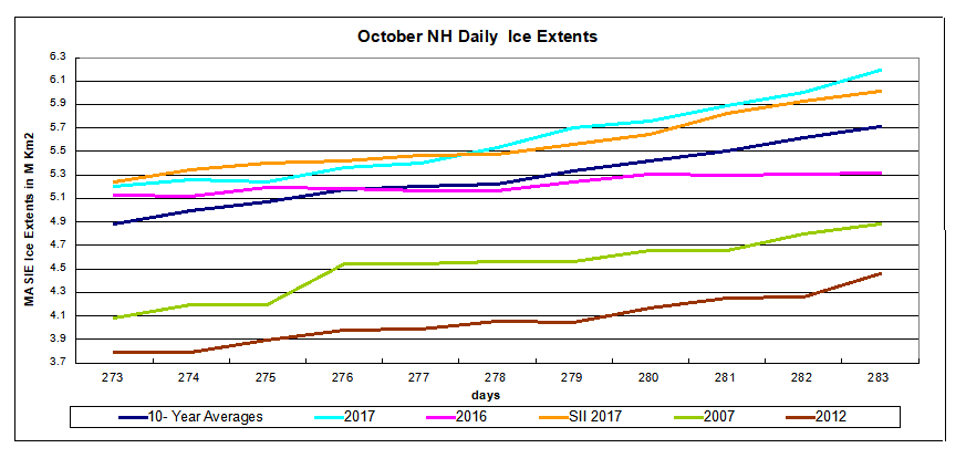
With five days left in the month, we can project the likely 2017 September results and compare with years of the previous decade. 2017 is provisional depending on the next five days, but MASIE is averaging 4.8M km2 and the daily extents are over that amount. SII is 60k km2 lower, but just went over 4.9M, so has a chance to also reach 4.8M.
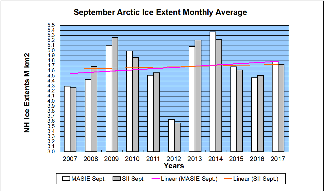
In August, 4.5M km2 was the median estimate of the September monthly average extent from the SIPN (Sea Ice Prediction Network) who use the reports from SII (Sea Ice Index), the NASA team satellite product from passive microwave sensors.
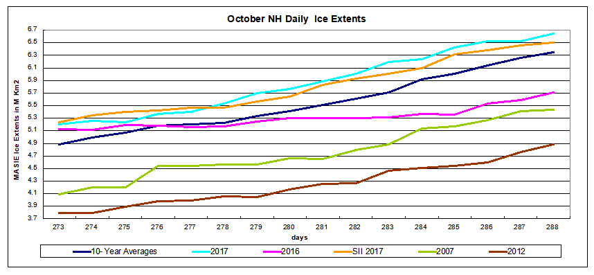
The graph below shows September comparisons through day 268.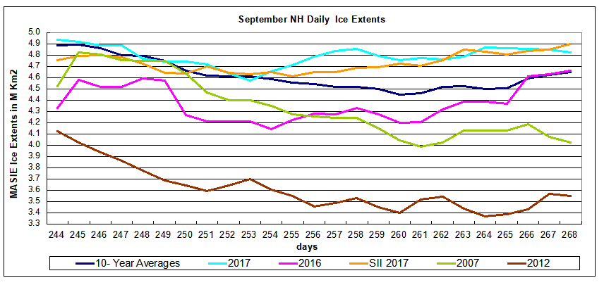 Note that as of day 260, 2016 had begun its remarkable recovery, now matching the 10 year average, nearly 200k km2 below 2017. Meanwhile 2007 is 800k km2 behind and the Great Arctic Cyclone year of 2012 is 1.3M km2 less than 2017. Note also that SII is currently showing slightly more ice than MASIE.
The narrative from activist ice watchers is along these lines: 2017 minimum is not especially low, but it is very thin. “The Arctic is on thin ice.” They are basing that notion on PIOMAS, a model-based estimate of ice volumes, combining extents with estimated thickness. That technology is not mature, and in any case refers to the satellite era baseline, which began in 1979.
The formation of ice this year does not appear thin, since it is concentrated in the central Arctic. Consider how CAA (Canadian Arctic Archipelago added 100k km2 in the last two weeks:

Click on image to enlarge.
The table shows ice extents in the regions for 2017, 10 year averages and 2007 for day 268. Decadal averages refer to 2007 through 2016 inclusive.
| Region |
2017268 |
Day 268
Average |
2017-Ave. |
2007268 |
2017-2007 |
| (0) Northern_Hemisphere |
4824033 |
4648420 |
175613 |
4025906 |
798128 |
| (1) Beaufort_Sea |
358982 |
488920 |
-129937 |
466599 |
-107617 |
| (2) Chukchi_Sea |
71545 |
180769 |
-109224 |
3054 |
68491 |
| (3) East_Siberian_Sea |
259179 |
276825 |
-17646 |
311 |
258868 |
| (4) Laptev_Sea |
275826 |
138290 |
137536 |
222968 |
52858 |
| (5) Kara_Sea |
42802 |
22613 |
20189 |
18246 |
24556 |
| (6) Barents_Sea |
6112 |
20560 |
-14448 |
4851 |
1261 |
| (7) Greenland_Sea |
111111 |
229228 |
-118116 |
335161 |
-224050 |
| (8) Baffin_Bay_Gulf_of_St._Lawrence |
74169 |
36672 |
37497 |
41385 |
32784 |
| (9) Canadian_Archipelago |
472601 |
293992 |
178610 |
274334 |
198267 |
| (10) Hudson_Bay |
1276 |
3154 |
-1878 |
1936 |
-661 |
| (11) Central_Arctic |
3149271 |
2956302 |
192969 |
2655784 |
493487 |
Note the strong surpluses in Canadian Archipelago and the Central Arctic, which is already at 95% of its March maximum. On the Russian side, Laptev and Kara are surplus to average, while East Siberian has grown to approach average.
Summary
Earlier observations showed that Arctic ice extents were low in the 1940s, grew thereafter up to a peak in 1977, before declining. That decline was gentle until 1994 which started a decade of multi-year ice loss through the Fram Strait. There was also a major earthquake under the north pole in that period. In any case, the effects and the decline ceased in 2007, 30 years after the previous peak. Now we have a plateau in ice extents, which could be the precursor of a growing phase of the quasi-60 year Arctic ice oscillation.

For context, note that the average maximum has been 15M, so on average the extent shrinks to 30% of the March high before growing back the following winter. In 2017 about 33% of the March maximum was retained, so the melt season losses were considerably less than in the past.
Background from Sept. 20
Dave Burton asked a great question in his previous comment, and triggered this response:
Dave, thanks for asking a great question. All queries are good, but a great one forces me to dig and learn something new, in this case a more detailed knowledge of what goes into MASIE reports.
You asked, where do they get their data? The answer is primarily from NIC’s Interactive Multisensor Snow and Ice Mapping System (IMS). From the documentation, the multiple sources feeding IMS are:
Platform(s) AQUA, DMSP, DMSP 5D-3/F17, GOES-10, GOES-11, GOES-13, GOES-9, METEOSAT, MSG, MTSAT-1R, MTSAT-2, NOAA-14, NOAA-15, NOAA-16, NOAA-17, NOAA-18, NOAA-N, RADARSAT-2, SUOMI-NPP, TERRA
Sensor(s): AMSU-A, ATMS, AVHRR, GOES I-M IMAGER, MODIS, MTSAT 1R Imager, MTSAT 2 Imager, MVIRI, SAR, SEVIRI, SSM/I, SSMIS, VIIRS
Summary: IMS Daily Northern Hemisphere Snow and Ice Analysis
The National Oceanic and Atmospheric Administration / National Environmental Satellite, Data, and Information Service (NOAA/NESDIS) has an extensive history of monitoring snow and ice coverage.Accurate monitoring of global snow/ice cover is a key component in the study of climate and global change as well as daily weather forecasting.
The Polar and Geostationary Operational Environmental Satellite programs (POES/GOES) operated by NESDIS provide invaluable visible and infrared spectral data in support of these efforts. Clear-sky imagery from both the POES and the GOES sensors show snow/ice boundaries very well; however, the visible and infrared techniques may suffer from persistent cloud cover near the snowline, making observations difficult (Ramsay, 1995). The microwave products (DMSP and AMSR-E) are unobstructed by clouds and thus can be used as another observational platform in most regions. Synthetic Aperture Radar (SAR) imagery also provides all-weather, near daily capacities to discriminate sea and lake ice. With several other derived snow/ice products of varying accuracy, such as those from NCEP and the NWS NOHRSC, it is highly desirable for analysts to be able to interactively compare and contrast the products so that a more accurate composite map can be produced.
The Satellite Analysis Branch (SAB) of NESDIS first began generating Northern Hemisphere Weekly Snow and Ice Cover analysis charts derived from the visible satellite imagery in November, 1966. The spatial and temporal resolutions of the analysis (190 km and 7 days, respectively) remained unchanged for the product’s 33-year lifespan.
As a result of increasing customer needs and expectations, it was decided that an efficient, interactive workstation application should be constructed which would enable SAB to produce snow/ice analyses at a higher resolution and on a daily basis (~25 km / 1024 x 1024 grid and once per day) using a consolidated array of new as well as existing satellite and surface imagery products. The Daily Northern Hemisphere Snow and Ice Cover chart has been produced since February, 1997 by SAB meteorologists on the IMS.
Another large resolution improvement began in early 2004, when improved technology allowed the SAB to begin creation of a daily ~4 km (6144×6144) grid. At this time, both the ~4 km and ~24 km products are available from NSIDC with a slight delay. Near real-time gridded data is available in ASCII format by request.
In March 2008, the product was migrated from SAB to the National Ice Center (NIC) of NESDIS. The production system and methodology was preserved during the migration. Improved access to DMSP, SAR, and modeled data sources is expected as a short-term from the migration, with longer term plans of twice daily production, GRIB2 output format, a Southern Hemisphere analysis, and an expanded suite of integrated snow and ice variable on horizon.
http://www.natice.noaa.gov/ims/ims_1.html
Footnote
Some people unhappy with the higher amounts of ice extent shown by MASIE continue to claim that Sea Ice Index is the only dataset that can be used. This is false in fact and in logic. Why should anyone accept that the highest quality picture of ice day to day has no shelf life, that one year’s charts can not be compared with another year? Researchers do this, including Walt Meier in charge of Sea Ice Index. That said, I understand his interest in directing people to use his product rather than one he does not control. As I have said before:
MASIE is rigorous, reliable, serves as calibration for satellite products, and continues the long and honorable tradition of naval ice charting using modern technologies. More on this at my post Support MASIE Arctic Ice Dataset