Residents view the first iceberg of the season as it passes the South Shore, also known as “Iceberg Alley,” near Ferryland, Newfoundland, Canada, April 16, 2017. REUTERS/Jody Martin

The title of this post sounds contradictory to most of what the media is saying about Arctic ice being in a tailspin, setting records for low extents, etc. And reports of ice blocking Newfoundland also fly in the face of media claims.

I will let you in on a secret: Arctic Ocean ice is doing fine and well above the decadal average. The only place where ice is below normal is outside the Arctic Ocean, namely Bering and Okhotsk Seas in the Pacific. Claims of disappearing ice pertain not to the Arctic itself, but to marginal Pacific seas that will melt out anyway by September.

I noticed the pattern this April when it became obvious that including Bering and Okhotsk in the Arctic totals gives a misleading picture. For sure they are part of Northern Hemisphere (NH) total sea ice, but currently the Pacific is going its own way, not indicative of the sea ice in the Central and Atlantic Arctic.

April 2017 is now complete. Focusing on the Arctic apart from Pacific marginal seas, remarkably the month ends with the same extent as it began at 13M km2. The graph below shows an early fluctuation down, followed by later gains and a gentle descent. May begins with the Arctic seas showing a surplus of ~400k km2 above average.

While the Arctic ocean ice is persisting, Bering and Okhotsk extents have retreated ahead of schedule, as the graph below shows.  Presently Bering and Okhotsk combined are 50% of decadal average, down by 500k km2.

The distinctive Pacific pattern is evident in the images of changing ice extents this April.  First, see how ice in Bering and Okhotsk seas has retreated steadily this month.

Meanwhile, on the Atlantic side ice has grown steadily.  Note the persistent ice blocking Newfoundland on the bottom right, and encasing Svalbard on the upper left.

The Chart below shows the traditional view of NH ice extents, which includes the Pacific seas together with the Arctic seas.  2017 is only slightly lower than average on this basis, despite a deficit of 500k km2 in Bering and Okhotsk, which obscures the ice surpluses elsewhere.  Comparisons with Sea Ice Index (SII) and 2007 are also shown.

Summary

The details are important to form a proper perception of any natural process, including dynamics of sea ice waxing and waning. On closer inspection, the appearance of declining Arctic sea ice is actually another after effect of the recent El Nino and Blob phenomena, and quite restricted to the Pacific marginal seas.

Meanwhile, on the Atlantic side of the Arctic, we have sightings and reports of ice surges along the coast of Newfoundland, such amounts not seen since the 1980s. Below an image of St. John’s harbour with tons of ice, provided by Ryan Simms.

And from Twillingate: “Basically it’s just an ocean of ice ahead of us.’ – Derrick Bath, Polar Venture

Derrick Bath’s Polar Venture has spent hours trying to make it through the ice near Twillingate. (Submitted by Danny Bath)

Heavy ice is making it impossible for fishermen from the Twillingate area to get to their crab fishing grounds. It may not open up until mid-May. (Twitter/@jeddore1972) Source: CBC

The title of this post sounds contradictory to most of what the media is saying about Arctic ice being in a tailspin, setting records for low extents, etc. And reports of ice blocking Newfoundland also fly in the face of media claims.

I will let you in on a secret: Arctic Ocean ice is doing fine and well above the decadal average. The only place where ice is below normal is outside the Arctic Ocean, namely Bering and Okhotsk Seas in the Pacific. Claims of disappearing ice pertain not to the Arctic itself, but to marginal Pacific seas that will melt out anyway in September.

I noticed the pattern this April when it became obvious that including Bering and Okhotsk in the Arctic totals gives a misleading picture. For sure they are part of Northern Hemisphere (NH) total sea ice, but currently the Pacific is going its own way, not indicative of the sea ice in the Central and Atlantic Arctic.

Graphically, MASIE shows that, excluding Bering and Okhotsk, 2017 Arctic Ocean sea ice is well above the 11 year average. Note that 2017 Arctic ice started April 100k km2 below average, and has now opened up a lead of ~300k km2 above average.

The second graph shows clearly how this year Bering and Okhotsk are abnormally low, and diverging further from average. At this point, Bering and Okhotsk combined are down to half of the decadal average.

The distinctive Pacific pattern is evident in the images of changing ice extents this April.  First, see how ice in Bering and Okhotsk seas has retreated steadily this month.

Meanwhile, on the Atlantic side ice has grown steadily.

The Chart below shows the traditional view of NH ice extents, which includes the Pacific seas together with the Arctic seas.  2017 is lower than average on this basis, though the difference is entirely due to Bering and Okhotsk, and obscures the ice surpluses elsewhere.  Comparisons with Sea Ice Index (SII) and 2007 are also shown.

The table for April 25, day 115 compares 2017 with the average (2006 to 2016), and with 2007 as the lowest year of the decade.

Note that all the central arctic seas are solid.  Barents is nearly average and much higher than 2007.  Baffin Bay-St.Lawrence is much above average and 2007, as shown by the Newfoundland ice that is part of the region.  The Bering and Okhotsk deficits are also obvious.

Summary

The details are important to form a proper perception of any natural process, including dynamics of sea ice waxing and waning. On closer inspection, the appearance of declining Arctic sea ice is actually another after effect of the recent El Nino and Blob phenomena, and quite restricted to the Pacific marginal seas.

Meanwhile, on the Atlantic side of the Arctic, we have sightings and reports of ice surges along the coast of Newfoundland, such amounts not seen since the 1980s. Below an image of St. John’s harbour with tons of ice, provided by Ryan Simms.

And from Twillingate: “Basically it’s just an ocean of ice ahead of us.’ – Derrick Bath, Polar Venture

Derrick Bath’s Polar Venture has spent hours trying to make it through the ice near Twillingate. (Submitted by Danny Bath)

As the photo shows, back in February 2017 you didn’t have to go looking for ice, it came after you. A convoy including icebreakers was trapped by ice in Chukchi, reported in Siberian Times and posted here as Arctic Ice Takes Revenge.

Now we are two weeks into April and about a month into the Arctic melt season. The hunt is on to see how ice extent reacts to the sun, warmer water and weather.

Firstly the graph shows that both this year and last have dipped below 14M km2, 400k km2 below average but still ahead of 2007. Day 104 refers to April 14.

As noted before, the heart of the Arctic is still frozen solid, with changes in extent occurring mainly in the marginal seas that usually melt out by September. Comparing the last two weeks in the Atlantic side, we can see almost no change overall, with an unexpected small increase in Barents Sea.

On the Pacific side is where the deficit to average appears in the melting of both Bering and Okhotsk Seas.

The table compares 2017 regional extents to average and to 2007.

Clearly, Barents is down slightly to average but more than offset by surpluses in Baffin and Greenland. The 2017 differences from average and from 2007 arise from Bering and Okhotsk in the Pacific.

Summary

Despite what you may hear from alarmist sources, there is plenty of Arctic Ice if you know where to look for it.

MASIE ice extents reported March 8 through 31, 2017.

This time of year the heart of the Arctic is frozen solid, and the only changes occur in the marginal seas.  Above shows the Atlantic basins, especially Kara, Barents, Greenland Sea and Baffin Bay.  All of them seesawed during the month, with some fall off at the end, especially noticeable in Gulf of St. Lawrence (counted with Baffin Bay).

Meanwhile on the Pacific side, Bering fluctuated, while Okhotsk lost extent steadily toward month end.

Context

The monthly ice extent average for March provides indication of any year’s annual maximum, prior to melting down to the September annual minimum. Sometimes a lower March extent yields a lower September extent, but not always: 2012 had both the highest maximum and lowest minimum in the last 11 years. That was the year of the Great Arctic Cyclone, and an outlier in the record.

Looking at the 11-year averages in the MASIE data set, the pattern in round numbers is:
Maximum: 15.0 M km2
Minimum: 4.8 M km2
Loss: 10.2 M km2
Loss: 68.0 % of maximum

So about 2/3 of the maximum extent is lost, varying from 66 to 70%. Obviously, all the factors affecting ice extents are in play: (Water, Wind and Weather) with the September outcome uncertain, but likely to be in the range observed.

March 2017 in Comparison

As has been reported, ice formation this year has been sluggish compared to other years. The graph below shows March 2017 compared with the 11 year average, and with 2006 and 2016, as well as SII (Sea Ice Index).

This March started below average, lost sllghtly until the third week, then recovered some before dropping off at the end. 2006 dropped off more rapidly than 2017, while 2016 ended near average. SII showed lower extents all month but drew close at the end.

The Table below shows Day 90 extents across the Arctic Seas compared to averages and 2006, the lowest recent year.

The marginal seas in the Atlantic and Pacific make the 2017 deficits to average: especially Barents, Kara, Bering and Okhotsk. Those seas usually lose all their ice by September. 2017 Surpluses in Greenland Sea and Baffin Bay are smaller, but make most of the difference with 2006.

2017 Outlook

March this year averaged 14.509 M Km2 compared to the 11 year average of 14.986 M km2, a deficit of 478k km2 or 3.2% down. That suggests that a typical melt later this year would result in a minimum of about 4.5 or 4.6 M km2, slightly down from the 11 year average of 4.8M km2.

Sea Ice Index (SII) typically shows less ice than MASIE, and SII reports a 2017 March average ice extent of 14.273 M km2 compared to SII 11 year March average of 14.842, a drop of 569k km2 or 3.8%.  Folks relying on SII may be expecting a lower September minimum, perhaps even breaking the present plateau of ice extents since 2007.  That remains to be seen.

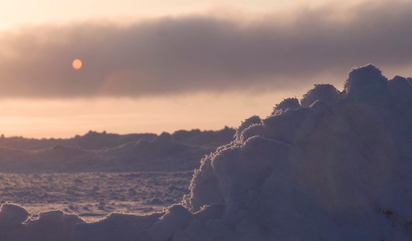
An early-spring sunset over the icy Chukchi Sea near Barrow (Utqiaġvik), Alaska, documented during the OASIS field project (Ocean_Atmosphere_Sea Ice_Snowpack) on March 22, 2009. Image credit: UCAR, photo by Carlye Calvin.

An earlier post Arctic Ice Factors discussed how ice extent varies in the Arctic primarily due to the three Ws: Water, Wind and Weather. There are other posts on the details of Water and Wind linked below at the end, but this post looks at some ordinary and repeating Weather events in the Arctic that influence ice formation. An interesting new study prompted this essay, but first some background on heat exchange observations in the Arctic.

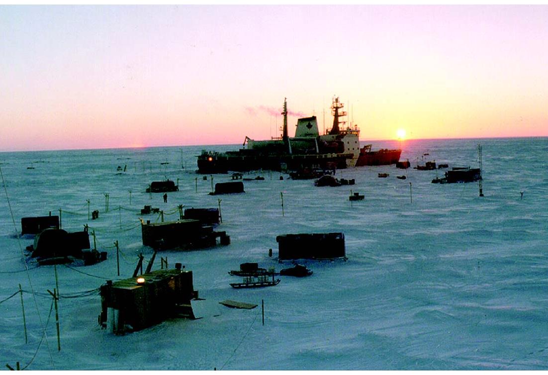
Ice Station SHEBA near the beginning of the drift on 28 October 1997. The Canadian Coast Guard Icebreaker Des Groseilliers served as a base of operations for the field experiment. The huts housed scientific equipment and logistical supplies.

One project in particular has provided comprehensive empirical data on the energy interface between Arctic Sea Ice and the atmosphere.  The SHEBA project collected heat exchange data on site in the Arctic as described in this article SHEBA: The Surface Heat Budget of the Arctic Ocean by Donald K. Perovich and John Weatherly, U.S. Army Engineer Research and Development Center, Cold Regions Research and Engineering Laboratory, Hanover, New Hampshire; and Richard C. Moritz, Polar Science Center, University of Washington, Seattle.

Overview

The combination of the importance of the Arctic sea ice cover to climate and the uncertainties of how to treat the sea ice cover led directly to SHEBA: the Surface Heat Budget of the Arctic Ocean. SHEBA is a large, interdisciplinary project that was developed through several workshops and reports. SHEBA was governed by two broad goals: understand the ice–albedo and cloud–radiation feedback mechanisms and use that understanding to improve the treatment of the Arctic in large-scale climate models. The SHEBA project was sponsored _jointly by the National Science Foundation’s Office of Polar Programs Arctic System Science program and the Office of Naval Research’s High Latitude Dynamics program.

Ice Station SHEBA

On 2 October 1997, the Canadian Coast Guard icebreaker Des Groseilliers stopped in the middle of an ice floe in the Arctic Ocean, beginning the year-long drift of Ice Station SHEBA. For the next 12 months, until 11 October 1998, Ice Station SHEBA drifted with the pack ice from 75°N, 142°W to 80°N, 162°W. At any given time, there were 20–50 researchers at Ice Station SHEBA. During the year over 200 researchers participated in the field campaign, spending anywhere from just a few days to the entire year. Conducting a year-long sea ice experiment provided daunting scientific and logistic challenges: low temperatures, high winds, ice breakup, demanding instruments, and polar bears.

There was an intense measurement program designed to obtain a complete, integrated time series of every possible variable defining the state of the “SHEBA column” over an entire annual cycle. This column is an imaginary cylinder stretching from the top of the atmosphere through the ice into the upper ocean. Observations included longwave and shortwave radiative fluxes; the turbulent fluxes of latent and sensible heat; cloud height, thickness, phase, and properties; energy exchange in the boundary layers of the atmosphere and ocean; snow depth and ice thickness; and upper ocean salinity, temperature, and currents. This year-long, integrated data set provides a test bed for exploring the feedback mechanisms and for model development.

The full set of observations is available in a report entitled Reconciling different observational data sets from Surface Heat Budget of the Arctic Ocean (SHEBA) for model validation purposes

All the detailed measurements are in the report, and the takeaway findings are summarized in Figure 8 below.

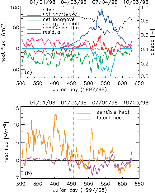
Figure 8. (a) Main components of the Surface Heat Budget of the Arctic Ocean (SHEBA) surface energy budget at the Pittsburgh site. (b) Sensible and latent heat fluxes (calculated using bulk formulations). The dashed line indicates the beginning of the summer (1 April), and the dotted line marks the onset of surface melt (29 May). Fluxes are smoothed using a 7 day running mean.

Figure 8a shows how the conductive heat flux in winter (October –March) is controlled by the net longwave radiation. The net longwave radiation has large variability. It is generally high for clear sky conditions, and low for cloudy sky, and constitutes a heat loss from the surface throughout the whole year. The net shortwave radiation (Figure 8a) is steadily growing in spring and early summer with a sudden increase in mid-June when the snow cover starts disappearing and the albedo drops to a lower value. When the surface temperature is at the melting point, the energy surplus is used for melting. This heat flux becomes the major counterbalance of the net solar flux during summer (April –September).

The sensible heat flux (Figure 8b) is usually small except in winter during clear sky conditions when the air temperature is relatively higher than the surface and the wind speed is higher [see Walsh and Chapman, 1998] (see Figure 1). In general, the surface is colder than the overlying air and the sensible heat is downward. During the winter,the sensible heat flux and the net longwave radiation are generally anticorrelated (Figures 8a – 8b). That is, the heat loss from the surface to the atmosphere during clear sky conditions leads to a positive temperature gradient in the air and results in a downward sensible heat flux. The coupling between these two fluxes is discussed in more detail by Makshtas et al. [1999]. The latent heat flux (Figure 8b) is close to zero except after the onset of the melt season when it has several peaks indicating moisture transport from the surface to the atmosphere. Figure 8a shows most components of the surface energy budget together, and the residual from all fluxes.

The Effects of Polar Weather Intrusions

With this background understanding of the winter heat flux over Arctic ice, let us consider the implications of the recent study.

An interesting paper analyzes intrusive weather and estimates the connection between such events and ice extents in the Arctic. The paper is:  The role of moist intrusions in winter Arctic warming and sea ice decline in Journal of Climate 29(12):160314091706008 · March 2016 by Cian Woods and Rodrigo Caballero, Department of Meteorology, and Bolin Centre for Climate Research, Stockholm University, Stockholm, Sweden

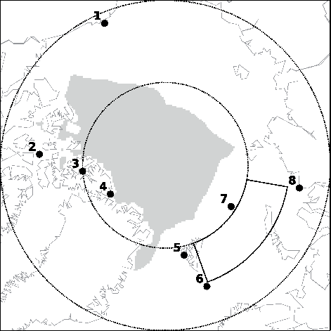
FIG. 1. Region with ONDJ SIC > 90% and trend < 2% decade-1 (gray shading). Numbered black dots show the location of the radiosonde stations: 1) Barrow, 2) Resolute, 3) Eureka, 4) Alert, 5) Ny-Ålesund, 6) Bjørnøya (Bear Island), 7) Polargmo (Heiss Island), and 8) Dikson Island. Solid black lines show the Barents Sea box (75°–80°N, 20°–80°E). Dotted lines indicate the 70° and 80°N latitude lines.

Abstract:

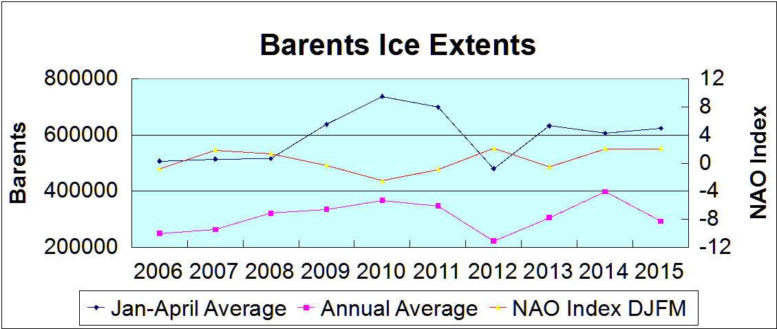
This paper examines the trajectories followed by intense intrusions of moist air into the Arctic polar region during autumn and winter and their impact on local temperature and sea ice concentration. It is found that the vertical structure of the warming associated with moist intrusions is bottom amplified, corresponding to a transition of local conditions from a ‘‘cold clear’’ state with a strong inversion to a ‘‘warm opaque’’ state with a weaker inversion. In the marginal sea ice zone of the Barents Sea, the passage of an intrusion also causes a retreat of the ice margin, which persists for many days after the intrusion has passed. The authors find that there is a positive trend in the number of intrusion events crossing 708N during December and January that can explain roughly 45% of the surface air temperature and 30% of the sea ice concentration trends observed in the Barents Sea during the past two decades.

An injection event is defined as a vertically integrated northward moisture flux across 708N in excess of 200 Tg day21 deg21 that is sustained for at least 1.5 days and occupies a contiguous zonal extent of at least 98 at all times.

The case study in Fig. 2 shows that the passage of an intrusion can induce local warming of over 20 K in the central Arctic. Here, we examine the typical thermodynamic impact of intrusions, focusing on the fully ice-covered interior of the Arctic basin—specifically, the region where monthly climatological SIC exceeds 90% and shows negligible trend across the data record. This region is shaded gray in Fig. 1.

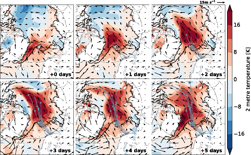
FIG. 2. Case study of an intrusion event beginning over northern Norway at 1800 UTC on 27 December 1999. Each panel shows a snapshot at a time relative to the beginning of the event as indicated in the lower-right corner. Gray lines show centroid trajectories with gray dots at 1-day intervals. Shading shows surface air temperature anomaly from a 6-hourly, smoothed seasonal cycle, arrows show 10-m wind, and the heavy black line shows the 15% SIC contour. As a reference, the dashed black line shows the 15% SIC contour 5 days before the beginning of the event. Dotted line is the 70°N latitude line. Thin black lines in the +5 days panel show the Barents Sea box.

An example intrusion event is shown in Fig. 2. The injection occurs over the northern tip of Norway and lasts for 1.75 days, yielding seven centroid trajectories. As the injection event progresses, its centroid shifts slowly eastward, giving some zonal spread in centroid trajectories. The flow field during the event features a large-scale dipole straddling the North Pole, with cyclonic circulation over the Atlantic/North American sector and an anticyclone over Eurasia. The trajectories reflect this structure, heading toward the North Pole after injection and then curving cyclonically to exit the Arctic over North America. The intrusion event is associated with large surface air temperature anomalies in the central Arctic and a retreat of the sea ice margin in the Barents Sea, topics we discuss in detail in sections 4 and 5 below.

To focus on intrusions that reach deep into the Arctic basin, events in which fewer than 40% of the trajectory ensemble members reaches 808N over 5 days are discarded. This leaves us with a final dataset of 359 intrusion events from 1990 to 2012, or ;16 per ONDJ season.

It is clear from Fig. 3 that by far the largest fraction of intrusions enters the Arctic through the Atlantic sector, with smaller numbers entering over the Labrador Sea and Greenland and from the Pacific. Interestingly, intrusions entering via the Atlantic and the Barents/Kara sector typically turn cyclonically toward North America—just as in the case study above—while those entering to the east of the Kara Sea typically turn anticyclonically and exit over Siberia. This suggests that moist intrusions into the Arctic are typically associated with cyclonic anomalies over eastern North America and anticyclonic anomalies over western Siberia, consistent with previous work.

Summary

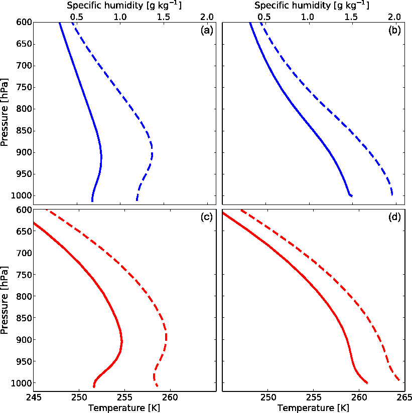
FIG. 5. (top) Humidity and (bottom) temperature profiles (left) in the ice-covered Arctic Ocean during ONDJ and (right) in the Barents Sea box during DJ. Solid lines show climatologies over the respective regions and seasons (representative of typical conditions in the absence of an intrusion event), and dashed lines show profiles at the time of maximum surface warming during a composite intrusion event (representative of conditions at the peak of the event).

A key feature of the warming trend in the Arctic is that it is bottom amplified (i.e., that it is in fact a trend toward a weakening of the climatological temperature inversion that prevails in ice-covered regions of the Arctic basin in winter). This feature has previously been mostly attributed to increased upward turbulent heat flux due to sea ice loss (Serreze et al. 2009; Screen and Simmonds 2010a,b).

Our results suggest a more nuanced view. The passage of an intrusion affects local conditions by inducing a transition from a “cold clear” state with a strong inversion to a “warm opaque” state with a much weaker inversion, in agreement with recent modeling work (Pithan et al. 2014; Cronin and Tziperman 2015). This yields an overall bottom-amplified local temperature perturbation, owing largely to surface heating by increased downwelling longwave radiation.

An increase in the frequency of intrusions can therefore drive bottom-amplified warming trend even in the absence of sea ice loss. In addition, the intrusions themselves drive sea ice retreat in the marginal zone and thus promote the upward turbulent fluxes that help produce bottom-amplified warming.

Our results agree with other recent work showing a strong impact of poleward moisture flux on Arctic sea ice variability and trends (D.-S. R. Park et al. 2015; H.-S. Park et al. 2015a,b). Since most of the moisture flux into the Arctic occurs in a small number of extreme events (Woods et al. 2013; Liu and Barnes 2015), it is natural to take an event-based approach as we do here, which allows us to study the structure of the intrusion events and their link to dynamical processes in the Arctic region and at lower latitudes.

Predicted surface air temperature trends (Fig. 9f) are greatest in the Barents Sea area extending into the central Arctic in agreement with observations (Fig. 9k), with the average trend predicted in the Barents Sea box approximately 45% of that observed. This localization of the trends arises both because intrusion counts have risen most rapidly in that region (Fig. 8b) and because individual intrusions have the greatest impact in that region (Fig. 9a). The predicted trend has a peak amplitude of about 3 K decade-1, about half of the observed value. For SIC the predicted trend (Fig. 9g) again coincides spatially with the observed trend (Fig. 9l) and peaks at about 10% decade, or about 1/3 the observed value at the same location, with the average predicted trend in the Barents Sea box being approximately 30% of that observed.

PS:

Current wind patterns over Barents and the Atlantic gateway to the Arctic can viewed at nullschool:
https://earth.nullschool.net/#current/wind/surface/level/orthographic=-6.21,74.48,522/loc=33.553,72.930

Footnote:

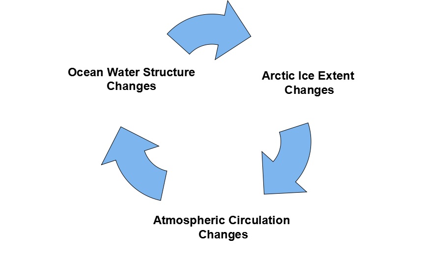
Arctic Sea Ice: Self-Oscillating System

Arctic Shifts between Cyclonic and Anticyclonic Wind Regimes The Great Arctic Ice Exchange

Drift ice in Okhotsk Sea at sunrise.

Previous posts have noted that in March, all the Arctic seas are locked in ice, the exceptions being Bering and Okhotsk in the Pacific, and Barents and Baffin Bay in the Atlantic. And the seesaw continues, shown in the images below.  Firstly on the Atlantic side, featuring Baffin Bay and Kara, Barents, Greenland Seas.

And on the Pacific side, the only action is in Bering and Okhotsk Seas.

The overall NH extents are down from the 11-year average, and it is mostly due to deficits in the usual places: Barents, Bering and Okhotsk, somewhat offset by a surplus in Baffin. All of them melt out in September, and Bering and Okhotsk basins are effectively outside of the Arctic ocean per se.

As reported previously, 2017 peaked early, rising close to the average on day 53 in February, then losing extent and never achieving the 15M km2 threshold.  14.8 M km2 proved to be the 2017 peak daily ice extent.  2016 also lost extent throughout March, though higher than the current year, and will likely end with a higher monthly average.  2006 and 2017 are virtually tied at this point, though 2017 will likely end up higher on the month.  SII shows about 300km2 less extent for the month, but drawing closer lately.

The Table below presents the ice extents reported by MASIE for day 80 in the years 2017, 2006 and the 11-year average (2006 through 2016).

The 2017 deficit to average is largely due to Okhotsk and Bering declining early, along with Barents and Kara.  A surplus in Baffin somewhat offsets these, especially in comparison with 2006.

To summarize, central Arctic seas are locked in ice, while extents have started to decline in the peripheral basins.  As of day 80, extents in 2017 are 4% below average and tied with 2006.

For ice extent in the Arctic, the bar is set at 15M km2. The average in the last 11 years occurs on day 73 at 15.07M before descending. Most years are able to clear 15M, except for 2006, 2007 and 2015 who topped out below that height.

Yesterday, March 2, 2016 cleared 15M, but will not reach that level again. 2016 will now drop down to 14.6M, rise to day 84 average of 14.9M, then start the descent into spring and summer. Typically, Arctic ice extent loses 67 to 70% of the March maximum by mid September, before recovering the ice in building toward the next March.

As reported previously, 2017 rose to the average in February, then lost extent for two days and is now increasing again.  The next two weeks will be interesting. The average year in the last eleven gained about 20k km2 from now to mid March. But the variability ranged from 2015 losing 350K while 2010 gained 300k km2. What will the ice do this year?  Where will 2017 rank in the annual Arctic Ice High Jump competition?

Drift ice in Okhotsk Sea at sunrise.

As reported previously, Arctic ice extents are solid in most seas, but continue to fluctuate at the margins. In the latter part of February 2017 there was a great leap upward for nine days, nearly reaching average and surpassing 2016, before falling back after day 53. The surplus over 2006 is now 500k km2. SII reports about 360k km2 less extent than MASIE.

The Atlantic upward leap and back in Barents and Baffin.

Note both Barents and Baffin pulled back slightly.

The Pacific shifting up and down in Bering and Okhotsk.

Note that Okhotsk continued to gain while Bering pulled back since day 53.

While the seesaws are tilting back and forth on the margins, the bulk of the Arctic is frozen solid. And with limited places where more extent can be added, the pace of overall growth has slowed.

The table below shows ice extents in the seas comprising the Arctic, comparing 2017 day 058 with the same day average over the last 11 years and with 2006.

The table shows that 2017 ice extent exceeds 2006 by about 500k km2 at this date. Surpluses are sizeable in Barents, Baffin and Okhotsk, with only the Baltic showing a deficit.  Baffin and Okhotsk are now average, and the 300k km2 deficit to average comes from Bering in the Pacific, and Barents and Greenland Seas on the Atlantic side

The big picture compares this day in 2017 with 2006.  Not much change overall, but a slight increase of 500k km2.

Drift ice in Okhotsk Sea at sunrise.

As reported previously, Arctic ice extents are solid in most seas, but continue to fluctuate at the margins. In the latter part of February 2017 there was a great leap upward for nine days, nearly reaching average and surpassing 2016, before falling back after day 53. The surplus over 2006 is now 500k km2. SII reports about 360k km2 less extent than MASIE.

The Atlantic upward leap and back in Barents and Baffin.

Note both Barents and Baffin pulled back slightly.

The Pacific shifting up and down in Bering and Okhotsk.

Note that Okhotsk continued to gain while Bering pulled back since day 53.

While the seesaws are tilting back and forth on the margins, the bulk of the Arctic is frozen solid. And with limited places where more extent can be added, the pace of overall growth has slowed.

The table below shows ice extents in the seas comprising the Arctic, comparing 2017 day 058 with the same day average over the last 11 years and with 2006.

The table shows that 2017 ice extent exceeds 2006 by about 500k km2 at this date. Surpluses are sizeable in Barents, Baffin and Okhotsk, with only the Baltic showing a deficit.  Baffin and Okhotsk are now average, and the 300k km2 deficit to average comes from Bering in the Pacific, and Barents and Greenland Seas on the Atlantic side

The next two weeks will be interesting. The average year in the last eleven gained about 100k km2 from now to mid March. But the variability ranged from 2015 losing 300K while other years gained 400k km2. What will the ice do this year?

The big picture compares this day in 2017 with 2006.  Not much change overall, but a slight increase of 500k km2.