Climate Scare in US South

A recent study published in Science predicts there will be no comfort for US southerners in the future.  As reported in the Atlantic

The American South Will Bear the Worst of Climate Change’s Costs
Global warming will intensify regional inequality in the United States, according to a revolutionary new economic assessment of the phenomenon.

The study, published Thursday in Science, simulates the costs of global warming in excruciating detail, modeling every day of weather in every U.S. county during the 21st century. It finds enormous disparities in how rising temperatures will affect American communities: Texas, Florida, and the Deep South will bleed income in the broiling heat, while some chillier northern states gain moderate benefits.

“We are really sure the South is going to get hammered,” says Solomon Hsiang, one of the authors of the paper and a professor of public policy at the University of California, Berkeley. “The South is really, really negatively affected by climate change, much more so than the North. That wasn’t something we were expecting going in.”

First of all, this comes from model projections, not from observed temperatures and precipitation.

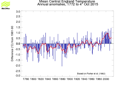
The graph shows daily maximums, averaged annually for the southern region as defined by the National Weather Service (NWS). The rise since 1895 is less than 1F, not even noticeable. You can also clearly see a quasi-60 year cycle, and that we are coming off the warmer phase with a cooler phase likely ahead.

Precipitation over the same period of 120 years shows a slight rise, nothing dramatic, and also oscillating with scattered peaks and valleys.

Secondly, all forecasting was done using the worst-case scenario

Out of five scenarios in IPCC report RCP8.5 is the most extreme. Neither AR5 nor the paper describing RCP8.5 call it a “business as usual” scenario, because it is not. Such a scenario would assume continuation of existing trends through 2100. A worst-case scenario assumes trends change for the worse. RCP8.5 assumes population growth at the 90th percentile of the probability forecast for 2100 (i.e., not considering real-world factors) and near-stagnation of technological progress.

Thirdly the models show no skill at all at regional forecasting, never mind their deficiencies at the global scale.

Roger Pielke Sr. repeatedly points to the elephant in the room about these papers — the ignored assumption that climate models’ predictions about global climate (when fed accurate predictions about emissions) are a sufficiently skillful basis for public policy — and that downscaling these models produces regional forecasts also useful for making public policy. There is little evidence of either. See here for a discussion of the literature about model validation (see the end section here for links to the literature). He says there is even less evidence for their skill at regional levels. He reviewed the literature validating regional downsizing five years ago, and relatively little progress has been made since then.
From Larry Kummer, US Economic Damage from Climate Change

Finally, and perhaps most importantly, Adaptation by humans is not allowed.

The projections presume that humans will not adapt in response to changing conditions, even though we have always done so, and presently have unprecedented capacities.

Matthew Kahn explains this clearly in Climate Change Adaptation Economics

An econometric research team follows the following recipe. First, it takes historical data and estimates how weather conditions correlate with economic conditions. For example, when it is extremely hot in a county — do we observe based on past data that the county’s per-capita income is lower than usual. The research team takes these past correlations and takes a climate change model (that tells you a guess of what will be future climate conditions by county) to predict future economic outcomes under the assumption that the historical correlation between weather and economic outcomes persists into the future.

This bold writing violates the Lucas Critique. Robert Lucas is one of the University of Chicago’s greatest economists. I was not one of his greatest students but I learned from him that as the “Rules of the Game” change that forward looking decision makers re-optimize. He studied this issue in the context of government counter-cyclical macro policy (i.e tax cuts during recessions) but the same point applies in the case of climate change. (my bold)

Let me explain;

Suppose it has always been 90 degrees in Phoenix in April but moving forward it will now be 105 degrees on average in Phoenix in April because of climate change. This is what I mean by a change in the Rules of the Game. The key stochastic process’ core parameters have changed. The climate scientists estimate such relationship using geocoded time series data. They spread their findings (through the New York Times and through wild bloggers such as Joe Romm).

Investors (those who invest in durable buildings, businesses, families) who live and work in a specific area such as Phoenix have strong incentives to take pro-active actions to reduce their exposure to hotter Aprils. They have thousands of adaptation strategies (and richer people have even more). One of the points I argue in Climatopolis is that induced innovation will take place because of Paul Revere style forecasts of hotter summers. Demand creates supply! I haven’t even mentioned government at the local, state or federal level. While many adaptation strategies are private goods (think of air conditioners), there are also public goods (sea walls, air cooling centers). If government changes its investments because of the new “Rules of the Game”, then the poor’s well being can improve in the face of a changing climate even if they can’t afford any of the private adaptation strategies. We are not passive victims here. The greatness of capitalism is that the set of alternatives we have to choose from keeps growing due to innovation and product differentiation. Each of these private and public goods helps us to individually and collective adapt.

As these changes takes place, the historical correlations between climate and economic losses are attenuated. This is why I don’t have much confidence in the predictions reported in the new Science Paper.

Summary

Alarmist blinders could not be more obvious. Their only solution is spending many trillions of dollars attempting to prevent future warming and climate change by reducing CO2 emissions (so-called “Mitigation”). The much more rational and time-honored policy of Adaptation would mean watching for changes and challenges to actually appear then mobilizing resources in response. But that would mean waiting because nothing is yet happening outside the normal range of temperatures and precipitation.   Unacceptable to true believers.

See also Climate Gloom and Doom

Glaciermania

A stream flows through the toe of Kaskawulsh Glacier in Yukon’s Kluane National Park. In 2016, this channel allowed the glacier’s meltwater to drain in a different direction than normal, resulting in the Slims River’s water being rerouted to a different river system..

The Weather Network (who do a decent job on local weather forecasting) are currently raving about Glaciers:

You know climate change is getting serious when rivers are resorting to piracy.

Canadian geomorphologist Dr. Daniel Shugar and his team headed to the Yukon last year to study changes in the flow of the Slims River, only to find out the river was gone.

The Slims, which was fed by the Kaskawulsh glacier, has become the victim of the first case of what’s known as river piracy in modern recorded history.

The team’s investigation soon turned up the culprit – the retreat of the Kaskawulsh Glacier, which has been retreating thanks to more than a century of climate warming.

What Actually Happened

Prior to May of last year, the glacier had been supplying water to two watersheds and feeding multiple rivers; the Kaskawulsh River, which drains to the Pacific Ocean via the Alsek River, and the Slims, which flowed north to the Bering Sea via Kluane Lake.

During the last days of May 2016, melt water at the base of the glacier finally managed to eat through the thinning ice sheet, opening a new canyon and sending the Slims’ share of the water into the Kaskawulsh instead.

Thanks to this abrupt change, water from the glacier that used to flow north to the Bering Sea has changed direction and flows toward the Pacific, instead, leaving the Slims basin high and (mostly) dry.

And Now, the Leap of Faith

In the published paper lead author Daniel Shugar goes on to state:
Based on satellite image analysis and a signal-to-noise ratio as a metric of glacier retreat, we conclude that this instance of river piracy was due to post-industrial climate change.

And others can’t resist piling on:

“To me, it’s kind of a metaphor for what can happen with sudden change induced by climate,” said John Clague, who holds a chair in natural hazard research at Simon Fraser University and was a co-author on the report.

“Climate change is happening, is affecting us and it’s not just about far-off islands in the South Pacific. .  Climate change may bring new changes that we’re not even really thinking about.” said Shugar.

It’s a nice PR touch to call this “Piracy”, but they are “jumping the shark” by claiming humans did this by burning fossil fuels.

“Jumping the shark” is attempting to draw attention to or create publicity for something that is perceived as not warranting the attention, especially something that is believed to be past its peak in quality or relevance. The phrase originated with the TV series “Happy Days” when an episode had Fonzie doing a water ski jump over a shark. The stunt was intended to perk up the ratings, but it marked the show’s low point ahead of its demise.

Hyping a Glacier retreating to prove global warming/climate change looks to be a similarly desperate move. Most people sense that the dynamics of glaciers growing, shrinking and moving is much more complex than simply fingering CO2 as the culprit.

south-glacier-as-seen-during-its-1986-surge-photo-p-johnson-and-in-2005-photo-g

FIG. 3. South Glacier as seen during its 1986 surge (photo: P. Johnson) and in 2005 (photo: G. Flowers). To facilitate comparison, the black line in each photograph marks the same feature.

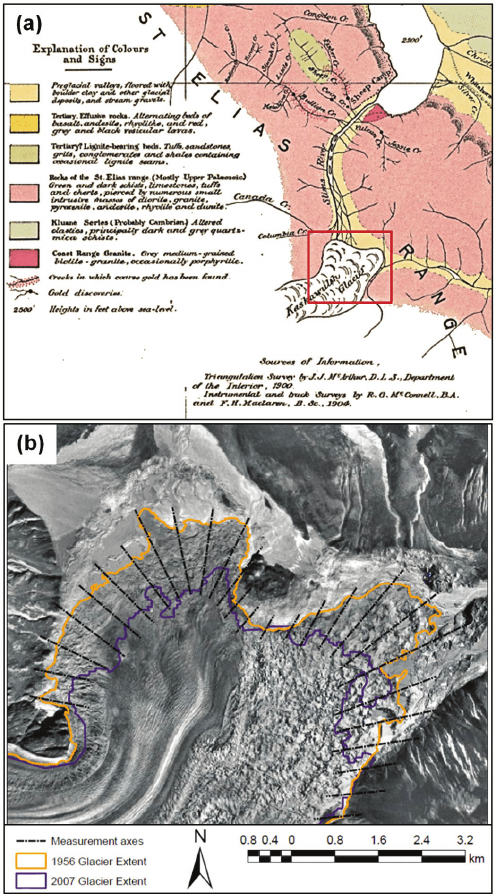
For context and scientific perspective we can turn to papers like this one:  Contemporary Glacier Processes and Global Change: Recent Observations from Kaskawulsh Glacier and the Donjek Range, St. Elias Mountains From the Abstract:

The scientific objectives of these projects are (1) to quantify recent area and volume changes of Kaskawulsh Glacier and place them in historical perspective, (2) to investigate the regional variability of glacier response to climate and the modulating inuence of ice dynamics, and (3) to characterize the hydromechanical controls on glacier sliding.

the-donjek-range-and-environs-geobase-r-image-8-september-2008-within-the-st-elias

FIG. 1. The Donjek Range and environs (Geobase ® image, 8 September 2008) within the St. Elias Mountains (NASA Aqua – MODIS image, 9 August 2003; North and South Glaciers are outlined, and locations of automatic weather stations operated since 2006 – 07 are marked with stars.

Excerpts (bolded text is my emphasis)

Kaskawulsh Glacier is ~70 km long from its shared accumulation area with the upper Hubbard Glacier, at an elevation of ~2500 m asl, to its terminus ~25 km southwest of the Kluane Lake Research Station, at ~820 m asl (Fig. 1). It provides the source of the Slims River, the primary water input for Kluane Lake to the northeast (which drains to the Bering Sea), and the source of the Kaskawulsh River to the southeast (which drains to the Gulf of Alaska).

One of the most iconic and best studied outlet glaciers of the St. Elias Mountains, Kaskawulsh Glacier was the focus of much glaciological research during the Icefield Ranges Research Project between the 1960s and early 1970s  and contemporary studies suggest that the glacier is temperate throughout. The current area of Kaskawulsh Glacier is ~1095 km2. Ice thicknesses range from 539 m near the topographic divide with the upper Hubbard Glacier and ~500 m at the confluence of the north and central arms at ~1750 m asl to 778 m at ~1600 m asl. The equilibrium line altitude is estimated from 2007 late summer satellite imagery as 1958 m asl, and it appears to have changed little since the 1970s.

The size of Kaskawulsh Glacier has varied considerably through time, with radiocarbon dating suggesting that it expanded by tens of kilometres into the Shakwak Valley (currently occupied by Kluane Lake) ~30 kya during the Wisconsinan Glaciation. In the historical past, Borns and Goldthwait (1966) mapped three sets of Little Ice Age moraines in the glacier forefield on the basis of distinctive variations in vegetation cover, morphology, and the ages of trees and shrubs.

Kaskawulsh Glacier was advancing by the early 1500s and reached its maximum recent position by approximately AD 1680. A recent study based on tree-ring dates suggests that the Slims River lobe reached its greatest Little Ice Age extent in the mid-1750s, whereas the Kaskawulsh River lobe reached its maximum extent around 1717. However, it appears that the glacier did not start retreating from this position until the early to middle 1800s. The recent discovery of a Geological Survey of Canada map of the glacier terminus from 1900 to 1904 indicates that the glacier was still in a forward position at that time, suggesting that most of the terminus retreat occurred in the 20th century.

Recent studies conducted by researchers at the University of Alaska and the University of Ottawa indicate that ice losses from Kaskawulsh Glacier have continued through the latter half of the 20th century and first decade of the 21st century, although evidence for any recent acceleration in loss rates is equivocal.

Global Context

Of the 19 glacierized regions of the world outside of the ice sheets, the region including the St. Elias Mountains made the second highest glaciological contribution to global sea level during the period 1961 – 2000. Only Arctic Canada is expected to exceed this region in sea-level contribution over the 21st century.

The St. Elias Mountains exhibit high interannual variability in ice mass change, which is due in part to the abundance of surge-type and tidewater glaciers in different stages of their respective cycles. Ice dynamics can be a confounding influence when attempting to isolate the effects of climate as an external driver of glacier change. For example, a surge-type glacier in the “quiescent” phase of its cycle may retreat even in a stationary climate. Catastrophic retreat of a tidewater glacier may be triggered by climate, but it is largely controlled by glacier and fjord geometry. Similar “flow instabilities” exist at larger scales in the form of ice streams and marine ice-sheets or outlet glaciers, the dynamics of which dominate the mass balances (and therefore sea-level contributions) of large sectors of the modern ice sheets. Our ability to project future changes on short (sub-decadal to decadal) timescales therefore hinges on our understanding of internal glacier dynamics, as well as our ability to project future climate in a given region and relate climate to glacier surface mass balance.

The ice-walled canyon at the terminus of the Kaskawulsh River in the Yukon, with recently collapsed ice blocks, that now carries the vast majority of glacier-front water down the Kaskawulsh Valley toward the Gulf of Alaska and the Pacific Ocean instead of north along the Slims River toward the Bering Sea. (Jim Best/University of Illinois)

Whether climate has fundamentally altered the surging styles of Trapridge Glacier and South Glacier from the faster, shorter, more recognizable Alaskan style to the slower and more subtle Svalbard style is an interesting question. Many small poly-thermal glaciers, whose temperate ice content is largely controlled by meltwater entrapment and refreezing in the accumulation area, are expected to become colder under negative mass balance conditions. It is therefore conceivable that thermal evolution over the course of decades can play a role in altering surge style. However, there is some evidence that both types of surges may be preceded by a prolonged—and until recently, unrecognized—period of acceleration. Thus, a “slow surge” or “partial surge” may simply represent a truncation of the ordinary surge cycle that results from a deficit of mass, rather than a fundamental change in surge character. Mass deficits have manifested themselves differently on the well-studied and temperate Variegated Glacier, where the return interval between surges adapts itself in such a way that surges are triggered at a constant cumulative balance threshold. The nature and timing of future surges of the large glaciers in the St. Elias Mountains will be instructive as we seek a more coherent understanding of the influence of climate on surging.

Summary

So it is a familiar story. A complex naturally fluctuating situation, in this case glaciers, is abused by activists to claim support for their agenda. I have a lot of respect for glaciologists; it is a deep, complex subject, and the field work is incredibly challenging. And since “glacial” describes any process where any movement is imperceptible, I can understand their excitement over something happening all of a sudden.

But I do not applaud those pandering to the global warming/climate change crowd. They seem not to realize they debase their own field of study by making exaggerated claims and by “jumping the shark.”
The lead authur, Shugar, sounds like a Michael Mann wannabe, putting out sound bites to please the naive journalists. Maybe he thinks there is a Nobel prize in it if he plays his cards right.

Meanwhile real scientists are doing the heavy lifting and showing restraint and wisdom about the limitations of their knowledge.

The Kaskawulsh River, as it exits the lower terminus of Kaskawulsh Glacier and lakes. ‘ JIM BEST

Fear Not for Permafrosty


The Permafrost Bogeyman is Back!

The Climate Scare of this Week is apparently melting permafrost.The Met Office warning on April 10:

Increased climate change risk to permafrost. Global warming will thaw about 20% more permafrost than previously thought, scientists have warned – potentially releasing significant amounts of greenhouse gases into the Earth’s atmosphere.

The researchers, from Sweden and Norway as well as the UK, suggest that the huge permafrost losses could be averted if ambitious global climate targets are met.

Lead-author Dr Sarah Chadburn of the University of Leeds said: “A lower stabilisation target of 1.5ºC would save approximately two million square kilometres of permafrost.

“Achieving the ambitious Paris Agreement climate targets could limit permafrost loss. For the first time we have calculated how much could be saved.”

The permafrost bogeyman has been reported before, been debunked, but will likely return again like a zombie that never dies. I have likened the climate false alarm system to a Climate Whack-A-Mole game because the scary notions keep popping up no matter how often you beat them down with reason and facts. So once again into the breach, this time on the subject of Permafrost.

Permafrost basics

I Travelled to the Arctic to Plunge a Probe Into the Melting Permafrost is a Motherboard article that aims to alarm but also provides some useful information.

The ground above the permafrost that freezes and thaws on an annual cycle is called the active layer. The uppermost segment is organic soil, because it contains all the roots and decomposing vegetation from the surface. Beneath the organic layer is the moist, clay-like mineral soil, which sits directly on top of the permafrost. The types of vegetation will influence the contents of the soil—but in return, the soil determines what can grow there.

Kholodov inserted probes into the layers of soil and the permafrost to measure its temperature, moisture content, and thermal conductivity. The air-filled organic layer is a much better insulator than the waterlogged mineral soil. So an ecosystem with a thicker organic layer, where there’s more vegetation, should provide better protection for the permafrost below.

On a warm morning in the boreal forests around Fairbanks, Loranty squeezed between two black spruce trees and motioned to all the woody debris scattered on the ground. “Here, where we have more trees and denser forests, we have shallower permafrost thaw depths.”

He grabbed a T-shaped depth probe and shoved it into the ground. It only sank about a handspan before it struck permafrost. “When you have trees, they provide shade,” he said, “and that prevents the ground from getting too warm in the summer.” So here, the permafrost is shallow, right beneath the surface.

Other vegetation, like moss, can also protect permafrost. “It’s fluffy, with lots of airspace, like a down coat,” Loranty explained, “and heat can’t move through it well, so it’s a good insulator.”

But 800km north on the tundra, close to the Arctic Ocean, there are no trees. It’s a less productive ecosystem than the forest and provides little insulation to the frozen ground. Here, low-lying shrubs, grasses, and lichens dominate underfoot. When I grabbed the depth probe and pushed it in, it sunk down a meter before it bottomed out because the permafrost was much deeper.

Permafrost Nittty Gritty

To really understand permafrost, it helps to listen to people dealing with Arctic infrastructure like roads. A thorough discussion and analysis is presented in Impacts of permafrost degradation on a road embankment at Umiujaq in Nunavik (Quebec), Canada By Richard Fortier, Anne-Marie LeBlanc, and Wenbing Yu

Fig. 1. Permafrost distribution and marine transgression in Nunavik (modified after Allard and Seguin 1987). Location of the 14 Inuit communities in Nunavik.

Following the retreat of the Wisconsin Ice Sheet about 7600–7300 years B.P. on the east coast of Hudson Bay (Hillaire–Marcel 1976; Allard and Seguin 1985) and about 7500– 7000 years B.P. in Ungava (Gray et al. 1980; Allard et al. 1989), the sea flooded a large band of coastline in Nunavik (Fig. 1). Glaciomarine sediments were then deposited in deep water in the Tyrrell and D’Iberville Seas (Fig. 1). Due to the isostatic rebound, once exposed to the cold atmosphere, the raised marine deposits were subsequently eroded and colonized by vegetation, and permafrost aggraded from sporadic permafrost to continuous permafrost with increasing latitude (Fig. 1).

A case study is presented herein on recent thaw subsidence observed along the access road to the Umiujaq Airport in Nunavik (Quebec). In addition to the measurement of the subsidence, a geotechnical and geophysical investigation including a piezocone test, ground-penetrating radar (GPR) profiling, and electrical resistivity tomography (ERT) was carried out to characterize the underlying stratigraphy and permafrost conditions. In the absence of available ground temperature data for assessing the causes of permafrost degradation, numerical modeling of the thermal regime of the road embankment and subgrade was also undertaken to simulate the impacts of (i) an increase in air temperature observed recently in Nunavik and (ii) the thermal insulation effect of snow accumulating on the embankment shoulders and toes. The causes and effects of permafrost degradation on the road embankment are also discussed.

Fig. 11. (a) GPR reflection profile carried out on 14 July 2006 in the field with the 100 MHz antennas at a fixed offset of 1 m. (b) Major reflectors identified on the GPR reflection profile. (c) Cross section of the ground based on the combined interpretation of the GPR reflection profile and model of electrical resistivity (Fig. 12c). Note the vertical exaggeration (1:5).

Values of thawing and freezing n-factors according to the surface conditions (Figs. 4 and 13) are given in Table 1. The gray road surface absorbs solar radiation in summer, inducing a higher surface temperature than air temperature and a higher thawing n-factor than the ones for the natural ground surface. The thawing n-factor is close to unity and the surface temperature is close to the air temperature in summer for the natural ground surface (ground surface boundaries Nos. 2, 3, and 4). Due to the absence of snow cover on the road surface, the freezing n-factor is close to unity. However, an increase in snow thickness leads to a decrease in the freezing n-factor (Fig. 13 and Table 1). We make the assumption that from one year to another there is no change in surface conditions due to climate variability and the thawing and freezing n-factors are constant.

Fig. 13. Cross section of the road embankment and subgrade showing the stratigraphy and boundary conditions used for the numerical modeling. The numbers between arrows refer to the ground surface boundaries (Table 1)

Only the governing equation of heat transfer by conduction taking into account the phase change problem was considered to simulate the permafrost warming and thawing underneath the road embankment. However, complex processes of heat transfer, groundwater flow, and thaw consolidation can take place in degrading permafrost. The development of a two dimensional numerical model of these coupled processes is needed to accurately predict the thaw subsidence based on the thaw consolidation properties of permafrost and to compare this prediction with the performance of the access road to Umiujaq Airport.

As expected from the design of thick road embankments in cold regions,the permafrost table has moved upward 0.9 m underneath the road embankment, preventing permafrost degradation (Fig. 14a). However, the permafrost is slightly warmer by a few tenths of degree Celsius underneath the road embankment than away from the road (Fig. 15). This increase in permafrost temperature due to the thermal effect of the road embankment makes the permafrost more vulnerable to any potential climate warming. The permafrost base in the bedrock has also moved upward 3.9 m for a permafrost thinning of 3 m (Fig. 15). This thawing taking place at the permafrost base does not induce any thaw settlement because the bedrock is thaw stable.

The subsidence is due to thaw consolidation taking place in a layer of ice-rich silt underneath a superficial sand layer. While the seasonal freeze–thaw cycles were initially restricted to the sand layer, the thawing front has now reached the thaw-unstable ice-rich silt layer. According to our numerical modeling, the increase in air temperature recently observed in Nunavik cannot be the sole cause of the observed subsidence affecting this engineering structure. The thick embankment also acts as a snow fence favoring the accumulation of snow on the embankment shoulders. The permafrost degradation is also due to the thermal insulation of the snow cover reducing heat loss in the embankment shoulders and toes.

Permafrost in Russia

Yakutsk Permafrost Institute Underground Lab

The Russians are seasoned permafrost scientists with Siberia as their preserve, and their observations are balanced by their long experience. The latest Russia report is from 2010.

We conclude the following based on initial analysis and interpretation of the data obtained in this project:

  • Most of the permafrost observatories in Russia show substantial warming of permafrost during the last 20 to 30 years. The magnitude of warming varied with location, but was typically from 0.5C to 2C at the depth of zero annual amplitude. This warming occurred predominantly between the 1970s and 1990s. There was no significant observed warming in permafrost temperatures in the 2000s in most of the research areas; some sites even show a slight cooling during the late 1990s and early 2000s.
  • Warming has resumed during the last two to three years at many locations predominantly near the coasts of the Arctic Ocean. Much less or no warming was observed during the 1980s and 1990s in the north of East Siberia. However, the last three years show significant permafrost warming in the eastern part of this region.
  • Permafrost is thawing in specific landscape settings within the southern part of the permafrost domain in the European North and in northwest Siberia. Formation of new closed taliks and an increase in the depth of preexisting taliks have been observed in this area during the last 20 to 30 years.

Methane Realism

An article in Scientific American raises several concerns about permafrost, but does add some realism:

First, while most of the methane is believed to be buried roughly 200 meters below the sea bed, only the top 25 meters or so of sea-bed are currently thawed, and thawing seems to have only progressed by about one meter in the last 25 years – a pace that suggests that the large bulk of the buried methane will stay in place for centuries to come.

Second, several thousand years ago, when orbital mechanics maximized Arctic warmth, the area around the North Pole is believed to have been roughly 4 degrees Celsius warmer than it is today and covered in less sea ice than today. Yet there’s no evidence of a massive amount of methane release in this time.

Third, the last time methane was released in vast quantities into the atmosphere – during the Paleocene-Eocene Thermal Maximum 56 million years ago – the process didn’t happen overnight. It took thousands of years.

Put those facts together, and we are probably not in danger of a methane time bomb going off any time soon.

Summary

The active layer of permafrost does vary from time to time and place to place. There was warming and some permafrost melting end of last century, but lately not so much. Any specific permafrost layer is influenced by many factors, including air temperatures, snow cover and vegetation, as well as the structure of the land, combining fill, sand, silt, ice and salinity mixtures on top of bedrock.

And nature includes negative feedbacks to permafrost melt. Any vegetation, even moss, growing in unfrozen soil provides insulation limiting further melting, as well as absorbing additional CO2. Reduced snowcover aids freezing and constrains later melting.

Rather than a permafrost bogeyman, we need a more people-friendly mascot. Consider our traditional nature friends loved by children and adults.

For example, Smokey the Bear

Rudolph the Reindeer

And the ever-popular Cola Bear

Introducing Permafrosty


Permafrosty is here!  Love him tender, and he’ll never let you down.

Additional Background on Permafrost in an earlier post The Permafrost Bogeyman


Banking on Climate Alarm

The media are again amping up claims of bad weather to be feared from “climate change.” It is Whack-A-Mole time again, so here is a complete debunking of such media reports, compiled to refute a particularly bad speech by Mark Carney Governor of the Bank of England. H/T Friends of Science

Fact Checking Mark Carney’s Climate Claims is a useful reference document written by Steven Kopits of Princeton Energy Advisors. A few examples below show his systematic dismantling of the alarmist narrative by referencing publically available sources, many of them on government or corporate sites.

Temperatures Rising


We do have long-time series data for Central England, extending back to 1772. To the extent this measurement is reliable and can be extrapolated to hemispheric averages, it shows a step-up of about 1 deg Celsius from 1980 to 2005, which supports Governor Carney’s assertions. On other hand, it also shows a drop of 0.5 deg Celsius from 2005 to the present—which does not.

Sea Levels

As with just about every other metric the Governor mentions, we have data. Sea level is measured by tide gauges, and also by satellites. Satellite measurements suggest that sea level has been rising steadily by roughly 3 mm / year, which equates to about 1 foot per century.

Weather-related Insurance Losses

SOURCE: MUNICH RE NATCAT SERVICE

Hurricanes account for 75% of catastrophic losses, with typhoons representing an additional 8%. Thus, hurricanes and typhoons represent $6 of every $7 paid out in ‘top ten’ catastrophic weather-related insurance claims.

And this in turn tells us a great deal about the nature of insurance. Where do insured hurricane losses occur? Principally in the United States. Where do insured typhoon losses occur? Principally in Japan and Taiwan. Why these places? Because all of these are wealthy countries. Hurricane and typhoon losses will be greater where there is, first, a concentration of physical assets, and second, where those assets are valuable. In other words, in the advanced countries exposed to hurricanes and typhoons.

In this, no country is more exposed than the United States. Of overall losses due to top ten catastrophic weather events, nearly 2/3 occurred in the United States alone.

Insured Weather-related Losses

SOURCE: MUNICH RE NATCAT SERVICE

Indeed, if we restrict this to insured losses (including floods and tornadoes), the US accounts for 84% by itself.  Thus, if we are speaking of insured weather-related losses, as a practical matter we are speaking of hurricane damage in the US.  The rest is largely incidental.  For example, Superstorm Sandy caused more insured losses in one event than the cumulative and collective top ten catastrophic, weather-related losses from Europe, China, and Japan since 1980.  And Sandy was only the second worst insurance event in recent times. 

Now, why are US losses so great? Is it due to the number or strength of storms making landfall in the United States?

GLOBAL HURRICANE FREQUENCY SOURCE: RYAN MAUE

In fact, there is no such pattern discernible in the data. Indeed, the last few years have seen fewer than average hurricanes globally, with a recovery to up-cycle numbers in the last year or so.

Rather, reinsurance data hints at the source of losses: higher payouts for assets in harm’s way. 

INSURED LOSSES AS A PERCENT OF OVERALL LOSSES, TOP TEN LISTS, 1980-2014 SOURCE: MUNICH RE NATCAT SERVICE

Further, more and more expensive assets are exposed to hurricanes in particular.  In the US, for example, ever more people are living on the coasts, and beach front property has become prized and expensive.  One need only look out the window on a flight approaching Miami International Airport to be appalled at the sheer concertation of high-end housing built just above sea level on islands dotting Florida’s Atlantic Coast.   How long until a hurricane wipes a good number of these off their foundations?  And what kind of insurance losses will that involve?

Indeed, an examination of catastrophic losses suggests a decisive role for government policy.  Hurricane Katrina, which destroyed New Orleans in 2005, represents alone more than one-quarter of all insured top ten losses globally since 1980.  In just one event. 

The article goes on to deal with other claims regarding Floods, Droughts, Tornadoes, and Wildfires before reaching this conclusion.

Summing Up

In his speech to London’s insurance community, Mark Carney, Governor of the Bank of England, asserted a series of claims about climate change. Some of these are widely accepted. The climate does change. The world has warmed. Atmospheric CO2 has increased, half of the increment due to human activities.

Beyond this, there is no consensus, and indeed, the available data in many cases directly refutes the Governor’s more extreme assertions. There is no consensus that humans are the primary drivers of climate change. As we can see, sea levels, for example, were rising well before the 1950s date Carney gives as the start of modern anthropogenic warming.

Importantly, the increase in losses since the 1980s is more likely to reflect expanded insurance coverage, increasing payouts as a percent of losses incurred, and an increased number of assets with higher values placed in harm’s way. Losses increases have not occurred due to increases in hurricane, tornado, flooding, drought or fire frequency or strength, at least not in the United States, which represents the lion’s share of insurance claims. In many cases, either frequency or intensity of weather-related events has actually declined. Sea level rise has not accelerated, not as measured by either satellites or tide gauges. Sea level has been rising for well over 100 years, and continues on that pace.

Like so many other economists, Governor Carney seems to operate under the assumption that current CO2 levels are just on the edge of some catastrophic acceleration. For some reason, 320 ppm of atmospheric CO2 is safe, but 540 ppm is not, because there is some precipice—an inflection point or boundary—between here and there. The limit is not 1,000 ppm, or 5,000 ppm, or 42,448 ppm, but right here, right now. A little more CO2, a trace more of a harmless trace gas, and we are doomed.

The climate is complex and the future uncertain. It is possible the worst fears may prove correct. Nevertheless, such an assertion is not supported by the historical data, not for US droughts, floods, tornados, hurricanes or fires. But it does show up. In politics. If sea levels were 20 cm higher in New York and this contributed to the damage from Superstorm Sandy, well, any middling analyst could have predicted the rise back in 1940, just as we can predict today that sea levels will be one foot higher a century hence. The failure was not of CO2 emissions, but squarely a failure of governance. And that goes doubly so for the fate of New Orleans. If Governor Carney wanted to make a constructive proposal, he should have called for Lloyds to create macro audits of risk zones and censure or refuse to insure jurisdictions where governance is not up to par. If insurers had refused to insure New Orleans unless the levees were sound, they could have saved themselves $30 bn in payouts and probably twice that in losses.

As an analyst, I find Mr. Carney’s speech is truly dismaying. For the Governor of the Bank to claim that climate change is leading to rapidly rising insurance claims is, at best, a critical failure of analysis. As discussed above, insurance claims are a function of a number of factors, including the type and country of the weather event, as well as the extent of insurance coverage and payout ratios. A hurricane in the US may see one hundred times the payouts of a major flood in India. Payouts will rise as a function of nominal GDP, as both inflation and the value and concentration of assets will play a crucial role in overall losses. The specific path of a storm can also be decisive for global averages. It goes without saying that a storm which strikes in Philadelphia, marches up the New Jersey coast, slams into the Manhattan and turns towards New Haven is going to cost a bundle. That same storm hitting, say, rural Mississippi would cause a fraction of the monetary damages. And this matters, because Superstorm Sandy caused more insured damages than all the leading weather events in Europe, Japan, and China combined. Single events can move long-term global averages.

If the Bank missed this, it is not because the necessary data is hard to find. Information on weather-related events is readily and publicly accessible on the internet. Almost every graph I use above relating to hurricanes, tornadoes, floods and droughts comes from the US government itself. Apparently, the Bank of England could not be bothered to consult the underlying climate data before making hyperbolic claims. Thus, at best, the Bank was careless with data analysis.

A worse interpretation of events suggests that Mr. Carney was willing to blindly accept the conventional wisdom, the ‘consensus of scientists’ regarding global warming, without any will or curiosity to dig deeper and form a personal view. One can only hope that monetary policy in the UK is not informed by such superficiality or passivity.

The very worst interpretation is that Mr. Carney is in fact aware of the source data, but chose to make hysterical claims to promote a personal political agenda. I cannot imagine a more ill-considered idea. For those of us who consider central bank independence sacred, the appearance of a national bank taking sides in a highly charged political debate—and doing so with scant regard for the underlying data—will establish the Bank of England as partisan and the political opponent of conservative politicians. Given that Janet Yellen, the Chairman of the US Federal Reserve Bank, hails from Berkeley, a hot bed of climate activism, should the Republican Party consider the Fed also its opponent? If so, I can assure you, the Republicans will find some support to ‘audit’ the institution.

At the end of the day, political neutrality is a pre-condition for central bank independence. If a political party deems the central bank to be an opponent, then it will take measures to gain political control over the bank, with the result that monetary policy itself may become politicized. If the Bank nevertheless feels compelled to champion a particular side in a political debate, its analysis must be water-tight and its communication, impartial. That Governor Carny violated both dictums is simply stunning and a huge blow to the prestige of the Bank of England. It was a very bad call indeed.

More anti-alarmist information at Climate Whack-A-Mole
https://rclutz.wordpress.com/2016/07/28/climate-whack-a-mole/

Greenland Viking Science


Eric the Red slept here: Qassiarsuk features replicas of a Viking church and longhouse. (Ciril Jazbec)

It is refreshing to come across scientists researching a question without the corrupting need to scare the public or to confirm some personal, professional or moral fear of the future. In this case I refer to a wonderful Smithsonian article on the question: Why Did Greenland’s Vikings Vanish? Newly discovered evidence is upending our understanding of how early settlers made a life on the island — and why they suddenly disappeared.

Some excerpts below give the flavor of this persistent effort by researchers unrewarded by the availability of huge grants that now flow to the once-lowly climatologists.  The whole article is fascinating to anyone with curiosity.

The Mystery of Greenland Vikings

But the documents are most remarkable—and baffling—for what they don’t contain: any hint of hardship or imminent catastrophe for the Viking settlers in Greenland, who’d been living at the very edge of the known world ever since a renegade Icelander named Erik the Red arrived in a fleet of 14 longships in 985. For those letters were the last anyone ever heard from the Norse Greenlanders.

They vanished from history.

Europeans didn’t return to Greenland until the early 18th century. When they did, they found the ruins of the Viking settlements but no trace of the inhabitants. The fate of Greenland’s Vikings—who never numbered more than 2,500—has intrigued and confounded generations of archaeologists.

Those tough seafaring warriors came to one of the world’s most formidable environments and made it their home. And they didn’t just get by: They built manor houses and hundreds of farms; they imported stained glass; they raised sheep, goats and cattle; they traded furs, walrus-tusk ivory, live polar bears and other exotic arctic goods with Europe. “These guys were really out on the frontier,” says Andrew Dugmore, a geographer at the University of Edinburgh. “They’re not just there for a few years. They’re there for generations—for centuries.”

So what happened to them?

The Conventional Wisdom

Thomas McGovern used to think he knew. An archaeologist at Hunter College of the City University of New York, McGovern has spent more than 40 years piecing together the history of the Norse settlements in Greenland. With his heavy white beard and thick build, he could pass for a Viking chieftain, albeit a bespectacled one. Over Skype, here’s how he summarized what had until recently been the consensus view, which he helped establish: “Dumb Norsemen go into the north outside the range of their economy, mess up the environment and then they all die when it gets cold.”

Thomas McGovern (with Viking-era animal bones); The Greenlanders’ end was “grim.” (Reed Young)

Accordingly, the Vikings were not just dumb, they also had dumb luck: They discovered Greenland during a time known as the Medieval Warm Period, which lasted from about 900 to 1300. Sea ice decreased during those centuries, so sailing from Scandinavia to Greenland became less hazardous. Longer growing seasons made it feasible to graze cattle, sheep and goats in the meadows along sheltered fjords on Greenland’s southwest coast. In short, the Vikings simply transplanted their medieval European lifestyle to an uninhabited new land, theirs for the taking.

But eventually, the conventional narrative continues, they had problems. Overgrazing led to soil erosion. A lack of wood—Greenland has very few trees, mostly scrubby birch and willow in the southernmost fjords—prevented them from building new ships or repairing old ones. But the greatest challenge—and the coup de grâce—came when the climate began to cool, triggered by an event on the far side of the world.

In 1257, a volcano on the Indonesian island of Lombok erupted. Geologists rank it as the most powerful eruption of the last 7,000 years. Climate scientists have found its ashy signature in ice cores drilled in Antarctica and in Greenland’s vast ice sheet, which covers some 80 percent of the country. Sulfur ejected from the volcano into the stratosphere reflected solar energy back into space, cooling Earth’s climate. “It had a global impact,” McGovern says. “Europeans had a long period of famine”—like Scotland’s infamous “seven ill years” in the 1690s, but worse. “The onset was somewhere just after 1300 and continued into the 1320s, 1340s. It was pretty grim. A lot of people starving to death.”

Amid that calamity, so the story goes, Greenland’s Vikings—numbering 5,000 at their peak—never gave up their old ways. They failed to learn from the Inuit, who arrived in northern Greenland a century or two after the Vikings landed in the south. They kept their livestock, and when their animals starved, so did they. The more flexible Inuit, with a culture focused on hunting marine mammals, thrived.

An aerial photograph of southern Greenland. (Ciril Jazbec)

New Evidence Overturns Past Conceptions

But over the last decade a radically different picture of Viking life in Greenland has started to emerge from the remains of the old settlements, and it has received scant coverage outside of academia. “It’s a good thing they can’t make you give your PhD back once you’ve got it,” McGovern jokes. He and the small community of scholars who study the Norse experience in Greenland no longer believe that the Vikings were ever so numerous, or heedlessly despoiled their new home, or failed to adapt when confronted with challenges that threatened them with annihilation.

“It’s a very different story from my dissertation,” says McGovern. “It’s scarier. You can do a lot of things right—you can be highly adaptive; you can be very flexible; you can be resilient—and you go extinct anyway.” And according to other archaeologists, the plot thickens even more: It may be that Greenland’s Vikings didn’t vanish, at least not all of them.

A New Understanding How Vikings Lived on Greenland


The Vikings established two outposts in Greenland: one along the fjords of the southwest coast, known historically as the Eastern Settlement, where Gardar is located, and a smaller colony about 240 miles north, called the Western Settlement. Nearly every summer for the last several years, Konrad Smiarowski has returned to various sites in the Eastern Settlement to understand how the Vikings managed to live here for so many centuries, and what happened to them in the end.

“Probably about 50 percent of all bones at this site will be seal bones,” Smiarowski says as we stand by the drainage ditch in a light rain. He speaks from experience: Seal bones have been abundant at every site he has studied, and his findings have been pivotal in reassessing how the Norse adapted to life in Greenland. The ubiquity of seal bones is evidence that the Norse began hunting the animals “from the very beginning,” Smiarowski says. “We see harp and hooded seal bones from the earliest layers at all sites.”

A seal-based diet would have been a drastic shift from beef-and-dairy-centric Scandinavian fare. But a study of human skeletal remains from both the Eastern and Western settlements showed that the Vikings quickly adopted a new diet. Over time, the food we eat leaves a chemical stamp on our bones—marine-based diets mark us with different ratios of certain chemical elements than terrestrial foods do. Five years ago, researchers based in Scandinavia and Scotland analyzed the skeletons of 118 individuals from the earliest periods of settlement to the latest. The results perfectly complement Smiarow­ski’s fieldwork: Over time, people ate an increasingly marine diet, he says.

Judging from the bones Smiarowski has uncovered, most of the seafood consisted of seals—few fish bones have been found. Yet it appears the Norse were careful: They limited their hunting of the local harbor seal, Phoca vitulina, a species that raises its young on beaches, making it easy prey. (The harbor seal is critically endangered in Greenland today due to overhunting.) “They could have wiped them out, and they didn’t,” Smiarowski says. Instead, they pursued the more abundant—and more difficult to catch—harp seal, Phoca groenlandica, which migrates up the west coast of Greenland every spring on the way from Canada. Those hunts, he says, must have been well-organized communal affairs, with the meat distributed to the entire settlement—seal bones have been found at homestead sites even far inland. The regular arrival of the seals in the spring, just when the Vikings’ winter stores of cheese and meat were running low, would have been keenly anticipated.

The Vikings Were Players in the Ivory Trade

The Norse harnessed their organizational energy for an even more important task: annual walrus hunts. Smiarowski, McGovern and other archaeologists now suspect that the Vikings first traveled to Greenland not in search of new land to farm—a motive mentioned in some of the old sagas—but to acquire walrus-tusk ivory, one of medieval Europe’s most valuable trade items. Who, they ask, would risk crossing hundreds of miles of arctic seas just to farm in conditions far worse than those at home? As a low-bulk, high-value item, ivory would have been an irresistible lure for seafaring traders.

After hunting walruses to extinction in Iceland, the Norse must have sought them out in Greenland. They found large herds in Disko Bay, about 600 miles north of the Eastern Settlement and 300 miles north of the Western Settlement. “The sagas would have us believe that it was Erik the Red who went out and explored [Greenland],” says Jette Arneborg, a senior researcher at the National Museum of Denmark, who, like McGovern, has studied the Norse settlements for decades. “But the initiative might have been from elite farmers in Iceland who wanted to keep up the ivory trade—it might have been in an attempt to continue this trade that they went farther west.”

A bishop’s ring and top of his crosier from the Gardar ruins. (Ciril Jazbec)

How profitable was the ivory trade? Every six years, the Norse in Greenland and Iceland paid a tithe to the Norwegian king. A document from 1327, recording the shipment of a single boatload of tusks to Bergen, Norway, shows that that boatload, with tusks from 260 walruses, was worth more than all the woolen cloth sent to the king by nearly 4,000 Icelandic farms for one six-year period.

Archaeologists once assumed that the Norse in Greenland were primarily farmers who did some hunting on the side. Now it seems clear that the reverse was true. They were ivory hunters first and foremost, their farms only a means to an end. Why else would ivory fragments be so prevalent among the excavated sites? And why else would the Vikings send so many able-bodied men on hunting expeditions to the far north at the height of the farming season? “There was a huge potential for ivory export,” says Smiarowski, “and they set up farms to support that.” Ivory drew them to Greenland, ivory kept them there, and their attachment to that toothy trove may be what eventually doomed them.

A New Theory Why Viking Greenland Settlements Failed

For all their intrepidness, though, the Norse were far from self-sufficient, and imported grains, iron, wine and other essentials. Ivory was their currency. “Norse society in Greenland couldn’t survive without trade with Europe,” says Arneborg, “and that’s from day one.”

Then, in the 13th century, after three centuries, their world changed profoundly. First, the climate cooled because of the volcanic eruption in Indonesia. Sea ice increased, and so did ocean storms—ice cores from that period contain more salt from oceanic winds that blew over the ice sheet. Second, the market for walrus ivory collapsed, partly because Portugal and other countries started to open trade routes into sub-Saharan Africa, which brought elephant ivory to the European market. “The fashion for ivory began to wane,” says Dugmore, “and there was also the competition with elephant ivory, which was much better quality.” And finally, the Black Death devastated Europe. There is no evidence that the plague ever reached Greenland, but half the population of Norway—which was Greenland’s lifeline to the civilized world—perished.

The Norse probably could have survived any one of those calamities separately. After all, they remained in Greenland for at least a century after the climate changed, so the onset of colder conditions alone wasn’t enough to undo them. Moreover, they were still building new churches—like the one at Hvalsey—in the 14th century. But all three blows must have left them reeling. With nothing to exchange for European goods—and with fewer Europeans left—their way of life would have been impossible to maintain. The Greenland Vikings were essentially victims of globalization and a pandemic.

Summary

So there is a climate angle to the story of Greenland Vikings. Unlike climate alarmists, these scientists looked deeper and found a more complicated truth. Of course, even this explanation is provisional, because we are talking about science, after all.

OLYMPUS DIGITAL CAMERA

Global Weather Oscillations

H/T to No Tricks Zone for posting (here) on the remarkable forecasting record of Global Weather Oscillations Inc. founded by David Dilley. The ability to predict storm activity demonstrates an understanding of earth’s climate system dynamics. The theory and supporting evidence are available to all in a free ebook Natural Climate Pulse

The heart of the matter seems to be Mr. Dilley’s extracting from very long term Milankovitch Cycles to determine decadal variations in weather activity. From the ebook pp. 16 ff.

Earth’s Natural Rhythm and Global Warming -Cooling Cycles

After researching various elements of the Milankovitch Cycles, Mr. Dilley found that specific sub-cycles which are called the “Lunisolar Precession” are a major factor in determining and maintaining the earth’s natural climate rhythm. It is the Lunisolar Precession that controls almost all of earth’s climate cycles, and it is well known throughout the climatological science community, that specific “Milankovitch Cycles” are the primary mechanism that controls glacial and interglacial periods on earth. If it were not for the gravitational tidal field of the moon, and the electromagnetic and gravitational tidal field of the sun, earth would spin out of control (ref: 23). It is these two bodies that keep earth’s orbit and tilt within certain limits, and provide earth’s climate cycles.

Mr. Dilley researched the Lunisolar Precession cycles for over 20 years, and correlated specific cycles to recurring cycles of climate. GWO incorporated his findings into climate – weather forecast models which provide a unique approach and extremely accurate long range cycle predictions for historical major earthquakes, regional hurricane landfalls many years in advance, historical floods, droughts, natural carbon dioxide cycles, global warming and global cooling cycles.

david-dilley-global-weather-cycles_image_16

Figure 16 shows the approximate 9-year Lunisolar gravitational cycle. It is this cycle that is a major contributor to earth’s climate cycles. (Created by Global Weather Oscillations Inc.)

During the 1998 Global Warming Peak, the warm pulse occurred from 1990-93 and again 2004-07,and warmed the Arctic waters below the ice caps up to 1 Degree Celsius above normal. The Arctic Boundary Current from the Atlantic provides the largest input of water, heat, and salt into the Arctic Ocean; the total quantity of heat is substantial, enough to melt the Arctic sea ice cover several times over.
Courtesy…Fate of Early 2000s Arctic Warm Water Pulse Aigor V. Polyakov, Vladmir A. Alexeeve et al, Bulletin of the American Meteorological Society, Vol. 92 Number 5, May 2011

david-dilley-global-weather-cycles_image_17

Figure 17 shows the North Atlantic warm water pulse (Ref:41) that enters the Arctic Ocean in coincidence with the 9-year Lunisolar Pulse shown as the red dots in Figure 16.(Created by Global Weather Oscillations Inc.)

Thus it can be seen that it is likely the approximate 9-year Lunisolar gravitational tidal pulse that sets up a rhythm or heartbeat for earth. During the recurring 230-year global warming cycles a very strong gravitation pulse acts like a plunger in the North Atlantic, causing a warm water pulse surge to enter the Arctic Ocean. It takes the warm water 13-years to circulate around the Arctic Ocean (Ref:43), gradually cooling during the period as it mixes with cooler water. It is this pulse that melts the Arctic Ice from the bottom up and eventually causes open waters to appear as melting continues during the lifespan of the pulse.

david-dilley-global-weather-cycles_image_18

Figure 18 Shows the United States temperatures (red line) from 1880 on the left to the year 2008. Notice an approximate 9-year temperature rhythm for temperatures in the United States. Note the peaks in temperatures every 8 to 10 years, which are very similar to the 9-year Lunisolar. (Created by Global Weather Oscillations Inc.)

The strongest pulses are separated by 72-years during the 230-year global warming episode. For instance, a very warm water pulse caused 10-years of warm global temperatures in the 1930s, and a second very warm pulse 72-years later caused 10-years of warm global temperatures from 1998 to 2008. This approximate 9-year pulse also corresponds closely with temperature pulses around the world. If we extend the Lunisolar Precession 9-year Pulse out to an approximate 230-year pulse (full moon cycle only shown here), we get a clear picture of the relationship of the Lunisolar pulse to global warming cycles which occur approximately every 230 years.

Summary

Any theory stands or falls on the success of its predictions about the subject system’s behavior. Dilley is earning respect for his understanding of earth’s climate system. We should also note that his analysis anticipates a cooling period in the next decades, something not foreseen by any climate model builder.

Followup post is  https://rclutz.wordpress.com/2017/02/08/amo-atlantic-climate-pulse/

Climate Poppycock

Definition
pop·py·cock ˈpäpēˌkäk/informal noun meaning nonsense.
Synonyms: nonsense, rubbish, claptrap, balderdash, blather, moonshine, garbage;

Origin: mid 19th century: from Dutch dialect pappekak, from pap ‘soft’ + kak ‘dung.’

This is obviously the linguistically correct term for most of the articles on climate published in the mainstream media. And it serves to describe perfectly the output from alarmist activists.

Exhibit A is provided by Ken Ward, leader of the “valve turners” and defendant facing felony charges in Washington state.

This week he succeeded to convince a juror to refuse him conviction because in his defense he “put up a map of Skagit County, about a third of which will be under water in 2050.”

I call “Poppycock.”  A study from U. of Washington came up with a range of 1″ to 18″ SLR by 2050 for coastal Washington state. Not only will that not flood the place, the range tells you they are shooting in the dark.

http://www.cses.washington.edu/db/pdf/moteetalslr579.pdf

For a deeper look into this phenomenon, see Post-Truth Climatism

CO2 Causes Earthquakes! Really?

earthquakegraph

Number of worldwide earthquakes with a magnitude of 7 or greater over the last two decades. British Geological Survey

From the “Headlines Claim, Details Deny” department comes this whopper regarding climate effects on seismic activity in Canada.

Natural disasters are expected to increase as climate change pushes global temperatures higher, and some scientists believe earthquakes will also become more frequent. Global News (here)

The alarm is sounded by one scientist, Bill McGuire, writing in the Guardian last fall:

“An earthquake fault that is primed and ready to go is like a coiled spring … all that is needed to set it off is – quite literally – the pressure of a handshake,” writes scientist Bill McGuire, author of Waking the Giant: How a changing climate triggers earthquakes, tsunamis, and volcanoes.

As usual with these alarmist pieces, if you bother to read the details in the text, you discover the headline is misleading or totally false. (“Fake News,” anyone?).

After quoting that scary claim, the article goes on to make numerous statements of fact contradicting Mr. McGuire.

While many parts of the country are prone to seismic activity, experts say Canadians shouldn’t worry about their city or town suddenly becoming a earthquake hot spot due to a warmer atmosphere.

Earthquakes rattle Canada thousands of times every year — there are an estimated 2,500 annually in Western Canada alone. Thanks to the Internet, social media and apps, we’re now more aware of the activity that has always commonly occurred.

“Climate change is not something that just started,” noted Christie Rowe, assistant professor in earth and planetary sciences at McGill University.

“All the earthquake patterns that we know of are basically [from] the last century. So the patterns that we know of are already happening in the climate changing world.”

“A lot of people think there’s suddenly an increase but it’s just that they’re getting a lot more coverage than they used to,” said Alison Bird, earthquake seismologist with the Geological Survey of Canada.

Climate change, “won’t generally cause more earthquakes to happen,” Bird said.

“No, climate change will not result in increased earthquake activity,” agreed Gail Atkinson, professor of earth sciences at Western University, in an email to Global News.

“The glaciers receded from the last ice age, which was considerable time ago — we’re talking about thousands of years,” said Bird. “Because the weight of those glaciers receding has been lifted, the ground is slowly moving up after having that weight removed from it, and you can have earthquakes because of that sort of thing. They tend to be quite small.”

While there may be more small events, Canada’s sparsely-populated Arctic is unlikely to suddenly see massive seismic activity.

Summary

Note the flip-flopping (equivocation) around the term “climate change”. When geologists and seismologists are speaking within their discipline, they are referring to natural changes over thousands of years. With activists “climate change” serves as code for CO2 causing global warming.

Reading the article again, it actually serves to debunk McGuire’s claims, except for the first paragraph or two. The journalist actually sought the views of level-headed experts and printed them for readers to have as context. The gruel is getting pretty thin for desperate alarmists.

thisguyisfalling2R. I. P.  Chicken Little.

More on counterfactual headlines at Headlines Claim, but Details Deny

Tornados: Blame them on La Niña

A tornado brews near El Reno, Okla., May 2013. A new study links the frequency of tornadoes and hailstorms in parts of the southern United States to ENSO, a cyclic temperature pattern in the Pacific Ocean. Credit: John Allen

Reported in Science Daily Frequency of tornadoes, hail linked to El Niño, La Niña

“We can forecast how active the spring tornado season will be based on the state of El Niño or La Niña in December or even earlier,” said lead author John Allen, a postdoctoral research scientist at the International Research Institute for Climate and Society (IRI).

Allen and his coauthors show that moderately strong La Niña events lead to more tornadoes and hail storms over portions of Oklahoma, Texas, Kansas and other parts of the southern United States. El Niño events act in the opposite manner, suppressing both types of storms in this area.

While the information can’t pinpoint when and where storms will wreak havoc, it will nevertheless be useful for governments and insurance companies to prepare for the coming season, Allen said.

The Tornado statistics are available from the Storm Prediction Center (here).

El Niño was in effect for 2015 and most of 2016.  2015 had 36 deaths, all but 10 of them between Dec. 23 and 26. This year there have been 17 deaths recorded. An average year is 80 tornado deaths.

TOP 5 GREATEST U.S. ANNUAL TORNADO DEATH TOLLS

RANK YEAR DEATHS
1) 1925 794
2) 2011 553
3) 1936 552
4) 1917 551
5) 1927 540

In 2011–a La Niña year– tornadoes killed more than 550 people, higher than in the previous 10 years combined. Hail storms and tornadoes cause an average estimated $1.6 billion in insured losses each year in the United States, according to the insurer Munich RE. Powerful, isolated events such as the 2011 Joplin, Missouri, tornado can smash that average. That storm alone caused several billion dollars in damage and killed 158 people.

Image: La Niña is characterized by unusually cold ocean temperatures in the central equatorial Pacific. The colder than normal water is depicted in this image in blue. During a La Niña stronger than normal trade winds bring cold water up to the surface of the ocean. Credit: NASA

Image: La Niña is characterized by unusually cold ocean temperatures in the central equatorial Pacific. The colder than normal water is depicted in this image in blue. During a La Niña stronger than normal trade winds bring cold water up to the surface of the ocean. Credit: NASA

Past studies that have relied on eyewitness records alone have had limited success, said Allen. “For example, previous work has shown a clear linkage between ENSO and winter activity, but spring–the season when most of tornadoes occur in the southern U.S.–remained an enigma until now,” Allen said.

To get around these challenges, the Columbia University team created indices derived from environmental conditions such as wind shear, temperature and moisture. Each is a key ingredient in severe storm formation, and each is influenced by ENSO. The scientists then verified the indices using available observational records.

Summary

If La Niña strengthens beyond its present near-neutral condition, look for more killer tornados in the SE United States.  But it is not the fault of CO2 or fossil fuels.

Footnote December 4

I want to be as careful as the authors not to overstate the certainty of their findings. (h/t comment by Les Johnson).  Tornados are mesoscale events with multiple contributing factors.  Researchers have concluded that ENSO sets environmental conditions that favor or disfavor tornado formation, i.e. increase or decrease the probabilities.

Michon Scott provides a more detailed description of the mechanism entitled El Niño and La Niña affect spring tornadoes and hailstorms at Climate.gov (here).

In these maps, purple indicates higher storm event frequency, and brown indicates lower storm event frequency. Specifics vary, but in general, springtime tornadoes and hailstorms are less frequent in the southern central United States during El Niño, and more frequent during La Niña.

The research showed that ENSO affects tornado and hailstorm frequency by influencing the position of the jet stream over North America. El Niño weakens the surface winds that carry warm, most air from the Gulf of Mexico over Texas and neighboring states. La Niña, in contrast, concentrates hot, humid air over the region. The heat and humidity over the southern Plains states sets up a strong north-south temperature gradient, which in turn favors storm formation.

El Niño/La Niña conditions often persist from winter into spring, the researchers found, so the ENSO state seen in December, January, and February can be used to predict tornado and hailstorm frequency for March, April, and May.

Tornado season and hail season don’t have set beginnings and endings. In general, tornado season peaks in Gulf Coast states in the spring, in the southern Plains in May and June, and in upper Midwest in June and July. . . But tornadoes can strike at any time of year. Severe hailstorms often strike between May and July, but can also occur at any time of year.

Stormy Climate Deception

Wikipedia: 2013 Pacific typhoon season summary. Even including super-typhoon Haiyan, 2013 was an average year.

Wikipedia: 2013 Pacific typhoon season summary. Even including super-typhoon Haiyan, 2013 was an average year. image is from commdiginews

Paul Driessen tells it like it is in this Town Hall article (here).  Some excerpts that struck me and some bolding that I added.

No Real-World evidence supports a “dangerous manmade climate change” thesis. In fact, a moderately warmer planet with more atmospheric carbon dioxide would hugely benefit crop, forest and other plant growth, wildlife and humans – with no or minimal climate effect. A colder planet with less CO2 would punish them. And a chillier CO2-deprived planet with less reliable, less affordable energy (from massive wind, solar and biofuel projects) would threaten habitats, species, nutrition and the poorest among us.

And yet, as Hurricane Matthew neared Florida on the very day the Paris climate accord secured enough signatures to bring it into force, politicians, activists and reporters refused to let that crisis go to waste.

Matthew was a powerful storm that left destruction and death in its wake, especially in impoverished Haiti. Its slow track up the southeastern US coastline pummeled the region with rain, flooding and more deaths. But it was a Category 1 hurricane with 75 mph winds when it made landfall in South Carolina October 8, and a post-tropical storm as it moved offshore from North Carolina a day later.

Despite the rain and floods, that makes a record eleven years since a major (Category 3-5) hurricane last made landfall in the United States (Wilma in October 2005). The previous record major hurricane hiatus was nine years, 1860-1869, according to NOAA’s Hurricane Research Division.

Only a charlatan would suggest that this record lull is due to rising atmospheric carbon dioxide levels. But plenty of alarmist charlatans claim that any violent or “unseasonal” storms are due to “too much” CO2.

Just as intolerable, United Nations “humanitarian and disaster relief” agencies were issuing “emergency appeals” for $120 million in “life-saving assistance” funds for the desperate Haitians. This after President Obama improperly diverted $500 million from an economic aid program set up to address disease epidemics – like the Zika and cholera cases that are rapidly rising in Haiti – to the UN’s Climate Action Fund. So Obama and the UN blame hurricanes and diseases on manmade climate change, but refuse to spend money they already have on a hurricane disaster, and instead beg for more money. Incredible!

It is clearly not climate change that threatens the poor. It is policies imposed in the name of preventing climate change that imperil poor, minority, blue-collar, farm and factory families.

The impacts of climate change obsession on developing nations would be far worse, if they bowed to President Obama’s suggestions and agendas. African nations, he has said, should “leapfrog” “dirty” fossil fuels and instead utilize their “bountiful” wind, solar, geothermal and biofuel resources. In practice, that would mean having expensive, intermittent electricity and growing biofuel crops on Africa’s nutrient-depleted, drought-stricken lands, with no fertilizer, mechanized farming equipment or GMO seeds.

That is racist. It reflects an elitist preference that the world’s poor should die, rather than emit carbon dioxide “pollution,” drive cars, build modern homes, or engage in other “unsustainable” practices.

Thankfully, few developing countries are listening to such nonsense. Instead, they are using oil, natural gas and especially coal, in ever-increasing amounts, to lift their people out of abject poverty – because the “climate-saving” Paris non-treaty imposes no restrictions on their use of fossil fuels.

Keeping fossil fuels in the ground really means depriving people of reliable, affordable electricity; prolonging unemployment and poverty; having no feed stocks for plastics and petrochemicals, except what might come from biofuels; and blanketing hundreds of millions of acres of farm, scenic and habitat areas with biofuel crops, 400-foot-tall wind turbines, vast solar arrays and new transmission lines.

When taxpayers, consumers, unemployed workers and poor families finally recognize these inconvenient truths, the world will be a far better place – with true freedom, justice and opportunity for all.