Fear Not For Fiji

Fiji Map from Turtle Airways Seaplanes. Fiji International Airport is at Nadi.
Published this month is an update on sea levels at Fiji, and thankfully the threat level can be dialed way down. (H/T Tallbloke) The Research Article: Our Oceans-Our Future: New Evidence-based Sea Level Records from the Fiji Islands for the Last 500 years Indicating Rotational Eustasy and Absence of a Present Rise in Sea Level by Nils-Axel Mörner, Paleogeophysics & Geodynamics, Stockholm, Sweden. Excerpts with my bolds.
Update Feb. 17 at bottom
Abstract:
Previously, no study in the Fiji Islands had been devoted to the sea level changes of the last 500 years. No serious prediction can be made unless we have a good understanding of the sea level changes today and in the past centuries. Therefore, this study fills a gap, and provides real observational facts to assess the question of present sea level changes.
There is a total absence of data supporting the notion of a present sea level rise; on the contrary all available facts indicate present sea level stability. On the centennial timescale, there was a +70 cm high level in the 16th and 17th centuries, a -50 cm low in the 18th century and a stability (with some oscillations) in the 19th, 20th and early 21st centuries. This is almost identical to the sea level change documented in the Maldives, Bangladesh and Goa (India).
This seems to indicate a mutual driving force. However, the recorded sea level changes are anti-correlated with the major changes in climate during the last 600 years. Therefore, glacial eustasy cannot be the driving force. The explanation seems to be rotational eustasy with speeding-up phases during Grand Solar Minima forcing ocean water masses to the equatorial region, and slowing-down phases during Grand Solar Maxima forcing ocean waster massed from the equator towards the poles.
Background
The Intergovernmental Panel on Climate Change [1] has claimed that sea level is rising and that an additional acceleration is soon to be expected as a function of global warming. This proposition only works if the present warming would be a function of increased CO2 content in the atmosphere (an hypothesis termed AGW from Anthropogenic Global Warming). On a longer-term basis, it seems quite clear, however, that the dominant factor of global changes in temperature is changes in solar variability [2-3]. Regardless of what actually is driving climate change and sea level changes, the proposition of a rapidly rising sea level grew to a mantra in media and politics. This initiated a flood of papers rather based on models and statistics, however, than on actual field observations.
The Fiji government will be the chair-nation at the next international climate conference; COP23 in Bonn in November 2017 [4]. This paper represents a detailed analysis of available field observation on sea level changes in the Fiji Islands over the last 500 Years.
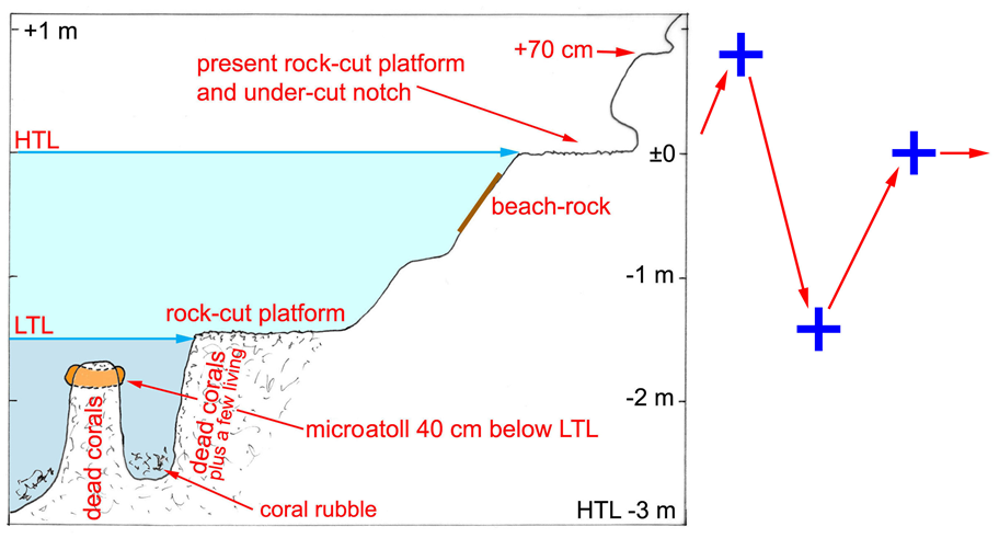
Figure 1.
Sea level changes as documented in the Yasawa Islands, Fiji, composed of 3 main segments: a high level (1), a low level (2) and a more or less constant level (3), which might be subdivided in an early high level, a main level just above the present level and a lowering to the present level generating microatoll growth in the last 60 years (based on data from [13]). (Subdivisions shown in Figure 3 below)

Figure 2.
The long-term changes during the last 500 years – i.e. a high, a low and a present level – is recorded in the Maldives [16], in Bangladesh [17-18] and in Goa, India, [15,18], as illustrated in Figure 3. A present long-term stability is also recorded in Qatar [19].

Figure 3.
The general agreement between the observed sea level changes in Fiji during the last 500 years, and those recorded in the three Indian Ocean sites: the Maldives, Goa and Bangladesh is striking, which is a very strong (even conclusive) argument that the recorded sea level change are of regional eustatic origin [20].
All four records show a high in the 17th century (which was a period of Little Ice Age conditions), a low in the 18th century (which was a period nearly as warm as today) and a high in the early 19th century (which was the last period of Little Ice Age conditions). This means that the Figure 3 sea level changes are almost directly opposite to the general changes in global climate. Consequently, the eustatic changes recorded cannot refer to glacial eustasy, but must be understood in terms of rotational eustasy.
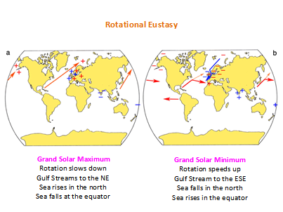
Figure 4
This calls for some explanation. The idea that oceanic water masses may be dislocated horizontally by rotational–dynamical forces was launched in 1984 [21] and more extensively presented in 1988 [22]. Later, is was proposed that changes in the Solar Wind strongly affects the Earth’s rate of rotation [23] (with a deeper analysis in [24]) leading to a beat in the Gulf Stream with alternations between a dominant northeastward flow during rotational slowing-down periods of Grand Solar Maxima, and dominant east-south eastward flow during rotational seeding-up periods of Grand Solar Minima [25].
The sea level changes in the Indian Ocean, were therefore proposed [26,15] to be driven by rotational eustasy; i.e. the interchanges of water masses between high-latitudes and the equatorial region as a function of the speeding-up during Grand Solar Minima with Little Ice Age conditions and slowing down during Grand Solar Maxima with generally warm climatic conditions.
In the post-Little Ice Ages period from 1850 up to 1930-1940 there was a global glacial eustatic rise in the order of 11 cm [28]. For the rest of the last 500 years, rotational eustasy seems to have been the dominant factor as documented in Figure 3 and illustrated in Figure 4.
CONCLUSIONS
(1)– sea level is not at all in a rising mode in the Fiji area
(2) – on the contrary it has remained stable in the last 50-70 years
(3) – rotational eustasy has dominated the sea level changes in Fiji
(4) – the same changes are recorded in the Indian Ocean
Previously, the changes in sea level during the last 500 years were not covered by adequate research in the Fiji Islands. The present paper provides a detailed analyses documenting a +70 cm high level in the 16th and 17th centuries, a -50 cm low in the 18th century and a period of virtually stability in the 19th to early 21st centuries, the last period of which may be subdivided into an early 19th century +30 cm high, a long period of stability and a 10-20 cm fall in sea level in the last 60 years forcing corals to grew into microatolls under strictly stable sea level conditions. This means there are no traces of a present rise in sea level; on the contrary: full stability.
The long-term trend is almost identical to the trends documented in the Indian Ocean in the Maldives, Goa and Bangladesh. This implies a eustatic origin of the changes recorded; not of glacial eustatic origin, however, but of rotational eustatic origin. The rotational eustatic changes in sea level are driven by the alternations of speeding-up during Grand Solar Minima (the Maunder and Dalton Solar Minima) forcing water towards the equator, and slowing-down during Grand Solar Maxima (in the 18th century, around 1930-1940 and at about 1970-2000).
Update Feb. 17
Prompted by a question from hunter, I found this informative recent letter on this topic (my bolds):
There are physical frames to consider. Ice melting requires time and heating, strictly bounded by physical laws. At the largest climatic jump in the last 20,000 years – viz. at the Pleistocene/Holocene boundary about 11,000 years BP – ice melted under extreme temperature forcing; still sea level only rose at a rate of about 10 mm/yr (or just a little more if one would consider more extreme eustatic reconstructions). Today, under interglacial climatic conditions with all the glacial ice caps gone climate forcing can only rise global sea level by a fraction of the 11,000 BP rate, which in comparison with the values of Garner et al. [1] would imply:
well below 0.4 m at 2050 instead of +0.6 m
well below 0.9 m at 2100 instead of +2.6 m
well below 2.9 m at 2300 instead of +17.5 m
Consequently, the values given by Garner et al. [1] violate physical laws and common glaciological knowledge. Therefore, their values must not be set as standard in coastal planning (point 2 above).
The mean sea level rise over the last 125 years is +0.81 ±0.18 mm/yr. At Stockholm in Sweden, the absolute uplift over the last 3000 years is strictly measured at +4.9 mm/yr. The mean tide-gauge change is -3.8 mm/yr, giving a eustatic component of +1.1 mm/yr for the last 150 years. In Amsterdam, the long-term subsidence is known as +0.4 mm/yr. The Amsterdam/Ijmuiden stations record a relative rise of +1.5 mm/yr, which give a eustatic component of +1.1 mm/yr.
Global Loading Adjustment has been widely used in order to estimate global sea level changes. Obviously, the globe must adjust its rate of rotation and geoid relief in close agreement with the glacial eustatic rise in sea level after the last Ice Age. The possible internal glacial loading adjustment is much more complicated, and even questionable, however.
Direct coastal analysis of morphology, stratigraphy, biological criteria, coastal dynamics, etc usually offers the far best means of recording the on-going sea level variations in a correct and meaningful way. It calls for hard work in the field and deep knowledge in a number of subjects. We have, very successfully, applied it in the Maldives, in Bangladesh, in Goa in southern India, and now also in the Fiji Islands. In all these sites, direct coastal analyses indicate full eustatic stability over the last 50-70 years, and long-term variations over the last 500 years that are consistent with “rotational eustasy” or “Global Solar Cycle Oscillations” (GSCO).