Climate Science | Science Matters

A Critical Framework For Climate Change

Posted on March 2, 2019 by Ron Clutz

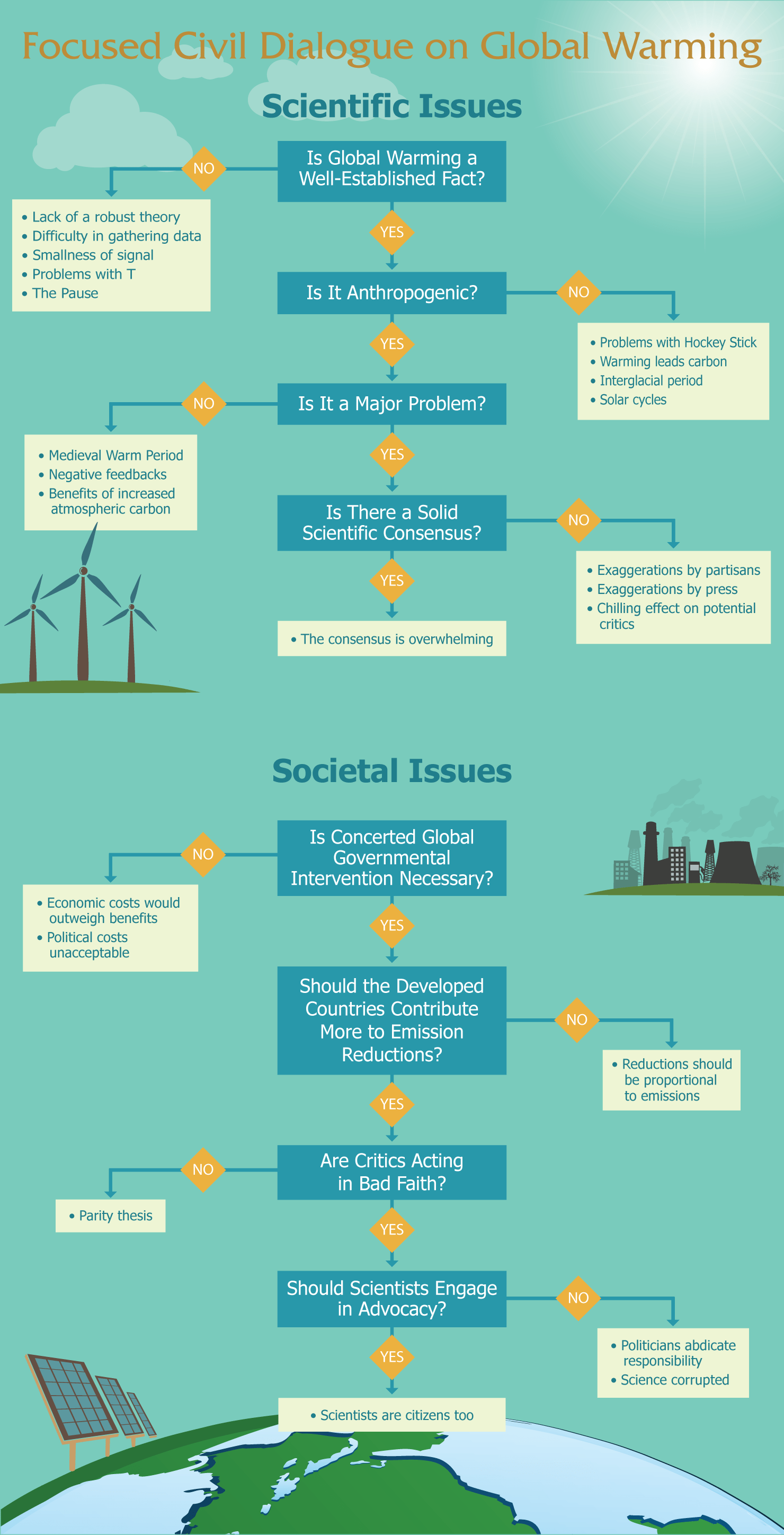
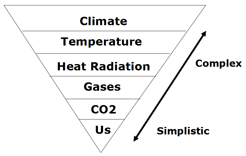
This dialogue framework was proposed for a debate between William Happer and David Karoly sponsored by The Best Schools. As you can see it reads like an high hurdle course for alarmists/activists. There are significant objections at every leap in connecting the beliefs.

Happer’s Statement: CO₂ will be a major benefit to the Earth

Earth does better with more CO2. CO2 levels are increasing

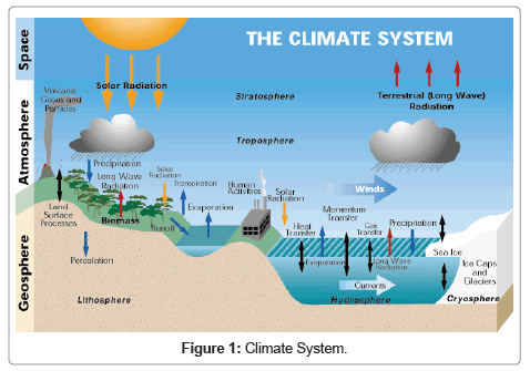
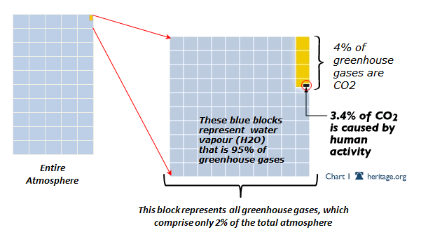
Atmospheric transmission of radiation: Tyndall correctly recognized in 1861 that the most important greenhouse gas of the Earth’s atmosphere is water vapor. CO2 was a modest supporting actor, then as now.

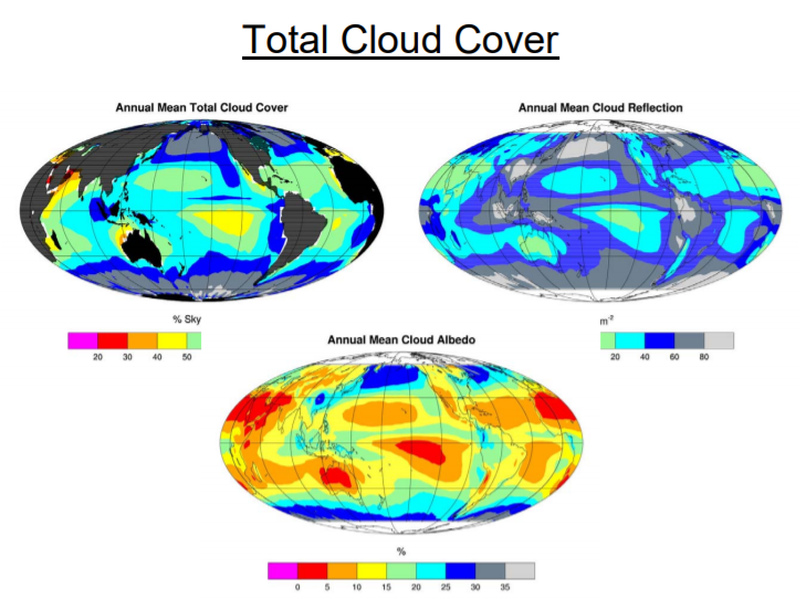
Radiative cooling of the Earth: Clouds are one of the most potent factors controlling Earth’ s surface temperature.

The Schwarzschild equation: The observed intensity I of upwelling radiation comes from the radiation emitted by the surface and by greenhouse gases in the atmosphere above the surface. The rate of change of the intensity with altitude is given by the Schwarzschild equation.

Logarithmic forcing by CO2: The intensity for a doubling of CO₂concentrations from the present value of 400 ppm to 800 ppm makes little difference, and simply leads to a slight broadening of the width of the band.

Convection: Radiation, which we have discussed above, is an important part of the energy transfer budget of the earth, but not the only part.

Numerical Modeling: Predictions about what more CO2 will do to the Earth’s climate are based on numerical modeling of the fluid flows in the atmosphere and oceans. Including water vapor, clouds, and precipitation further complicates the modeling considerations outlined above. Climate model builders have a hard job.

Equilibrium Climate Sensitivity: If increasing CO₂ causes very large warming, harm can indeed be done. But most studies suggest that warmings of up to 2 K will be good for the planet. More than a century after Arrhenius, and after the expenditure of many tens of billions of dollars on climate science, the official value of S still differs little from the guess that Arrhenius made in 1912: S = 4 K. Could it be that the climate establishment does not want to work itself out of a job?

Overestimate of S: Contrary to the predictions of most climate models, there has been very little warming of the Earth’s surface over the last two decades. If one assumes negligible feedback, where other properties of the atmosphere change little in response to additions of CO2, the doubling efficiency can be estimated to be about S = 1 K. The much larger doubling sensitivities claimed by the IPCC, which look increasingly dubious with each passing year, are due to “positive feedbacks.”

Benefits of CO2: More CO2 in the atmosphere will be good for life on planet earth. Few realize that the world has been in a CO2 famine for millions of years — a long time for us, but a passing moment in geological history.

More bogeymen: The earth has stubbornly refused to warm nearly as much as demanded by computer models. To cope with this threat to full employment, the climate establishment has invented a host of bogeymen, other supposed threats from more CO2. One of the bogeymen is that more CO2 will lead to, and already has led to, more extreme weather, But extreme weather is not increasing. We also hear that more CO2 will cause rising sea levels to flood coastal cities, large parts of Florida, tropical island paradises, etc.

Climate Science: Too much “climate research” money is pouring into very questionable efforts, like mitigation of the made-up horrors mentioned above. It reminds me of Gresham’s Law: “Bad money drives out good.”

Summary

The Earth is in no danger from increasing levels of CO2. More CO2 will be a major benefit to the biosphere and to humanity.

Karoly’s Statement: Climate change is harming nature and humanity

1. Observed global warming is beyond reasonable doubt

2. Increases in greenhouse gases are due to human activity

3. Most of the observed global warming since the mid-twentieth century is due to human activity

4. Global warming will continue over the twenty-first century

5. Many adverse impacts result from global warming

6. Substantial reductions in greenhouse gas emissions are needed to minimize dangerous global warming

Summary

The key points presented above are just a small fraction of the vast body of evidence that support the scientific conclusions on global warming accepted by all the scientific Academies and by all the governments around the world.

Science has established that it is virtually certain that increases of atmospheric CO2 due to burning of fossil fuels will cause climate change that will have substantial adverse impacts on humanity and on natural systems. Therefore, immediate stringent measures to suppress the burning of fossil fuels are both justified and necessary.

Happer’s detailed response to Karoly on climate change

Dr. Karoly begins his Statement, not with evidence to support the title, “Climate change is harming nature and humanity,” but with a summary of what happened in the “21st Conference of Parties to the United Nations Framework Convention on Climate Change in December of 2015.” What a mouthful!

As I pointed out in my Interview and Statement, there is no scientific evidence that global greenhouse gas emissions will have a harmful effect on climate. Quite the contrary, there is very good evidence that the modest increase in atmospheric CO2 since the start of the Industrial Age has already been good for the Earth and that more will be better.

Some climate scientists, including Dr. Karoly, are doing praiseworthy work. I especially admire high-quality, year-by-year measurements of properties of the atmosphere and oceans. But if they have doubts about climate hysteria, most practicing climate scientists keep these to themselves because of the ferocity of the attacks they know will come to those who question the party line.

In my Interview, I mentioned the attacks on me by Greenpeace. No wonder there is a consensus of climate scientists, or that few scientists from other fields are willing to question the established dogma! Even though creative scientists are not greatly impressed by them, claims of consensus work wonders with educated elites.

A brief discussion of those key points of Dr. Karoly’s Statement with which I disagree:

3. “The observed large-scale increase in surface temperature across the globe since the mid-twentieth century is primarily due to human activity, the increase of greenhouse gases in the atmosphere, and other impacts on the human climate system.” This statement is based on excessive faith in computer models.

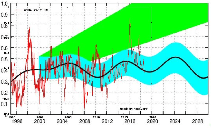
Trends in global mean surface temperature. a. 1993-2012. b. 1998-2012. Histograms of observed trends (red hatching) are from 100 reconstructions of the HadCRUT4 dataset. Histograms of model trends (grey bars) are based on 117 simulations of the models, and black curves are smoothed versions of the model trends. The ranges of observed trends reflect observational uncertainty, whereas the ranges of model trends reflect forcing uncertainty, as well as differences in individuals model responses to external forcings and uncertainty arising from internal climate variability.

4. “There will continue to be significant global warming over the 21st century with its magnitude depending on the emissions of greenhouse gases from human activities.” Again, this is a statement based on computer models. No one knows how the temperature of the Earth will change over the twenty-first century. It is just as likely that the Earth will cool, since whatever mechanism caused the Little Ice Age could act again and could overwhelm the small warming expected from increased CO2. In both my Statement and my Interview, I pointed out how much most models overestimated the warming of the Earth since the year 2000, when there was a hiatus or pause in warming, which may not be over yet.

5. “There are substantial adverse impacts on human and natural systems from global warming.” I disagree. I don’t know of a single adverse impact that can be confidently ascribed to more CO2. There are plenty of phony claims of damage, which quickly fall apart when scrutinized.

6. “Rapid, substantial, and sustained reductions in greenhouse gas emissions from human activities are needed to slow global warming and stabilize global temperature at a level that would minimize dangerous human influence on the climate system.” I disagree. We are being exhorted to “reduce our carbon footprint,” although to Dr. Karoly’s credit, he does not use this silly slogan. To the extent that “carbon footprint” includes soot (small particles of elemental carbon), and CO, carbon monoxide molecules, I would be glad to be part of the crusade.

General Comments

My Statement had 64 citations. I, too, cited many government reports, including those of the IPCC, but I also cited at least 16 peer-reviewed papers by independent scientific researchers. Dr. Karoly’s overwhelming focus on government reports looks like fully developed groupthink. Or maybe it is better described by the old Russian proverb:

Сила есть, ума не надо.

We have power, no need for intelligence.

Trotsky refers to the old principle which St. Paul states in 2 Thessalonians chapter 3:10 “We gave you this rule: if a man will not work, he shall not eat.” And before that Deuteronomy 25:4: “Do not muzzle an ox while it is treading out the grain.”

Enormous imagination has gone into showing that increasing concentrations of CO2 will be catastrophic. Cities will be flooded by sea-level rises that are 10 or more times bigger than even the IPCC predicts. There will be mass extinctions of species; billions of people will die; “tipping points” will render the planet a desert.

If you wrote down all the ills attributed to global warming, you would fill up a very thick book. And all of this despite the fact that in the history of higher life forms on Earth (the Phanerozoic), CO2 levels were four or more times higher than today, but life nevertheless flourished at least as abundantly on land and in the sea as it does today. It’s an ill wind, indeed, that blows no good.

In summary, Dr. Karoly is a good scientist who means well. But he lives in an echo chamber of like-minded people who are convinced that they are saving the world.

The scholars of the floating island of Laputa had much in common with many promoters of global-warming alarmism

No “Gold Standard” Climate Science

Posted on February 27, 2019 by Ron Clutz

Claims this week that climate scientists have “5-sigma” certainty for their findings are pure hype and extremely false adverrtising. Lubos Motl explains at his website Reference Frame “Five-sigma proof” of man-made climate change is complete nonsense Excerpts in italics with my bolds.

Notorious climate fearmonger Gavin Schmidt tweeted the following:

40 years since:
– the Charney report
– Hasselmann’s paper on detection & attribution
– the satellite erahttps://rdcu.be/bowzn @NatureClimate

Put it together and what have you got?
Greater than 5σ detection of anthropogenic climate change.

Lubos Motl:

He picks about 3 scientific teams and praises them for reaching the “gold standard” of science (which is how the journalists hype it) – a five-sigma proof of man-made global warming. The signal-to-noise ratio has reached some critical threshold, it’s those five sigma, so the man-made climate change is proven at the same level at which we needed e.g. the Higgs boson to be discovered by CERN’s particle physicists.

It sounds great except it’s complete nonsense. When we discover something at five sigma, it means something that clearly cannot be the case in climatology. When we discover new physics at five sigma, it means that we experimentally rule out a well-defined null hypothesis at the p-level of 99.9999% or so. Note that a “well-defined null hypothesis” is always needed to talk about “five sigma”.

In the case of the man-made climate change discussion, there is clearly no such “well-defined null hypothesis”. In particular, when Schmidt and others discuss the “signal-to-noise ratio”, they don’t really know what part of the observed data is “noise” and how strong it should be. The assumption must be that the “noise” is some natural variability of the climate. But we don’t really have any precise enough and canonical enough model of the natural variability. The natural variability is undoubtedly very complex and has contributions from lots of natural and statistical phenomena and their mixtures. Cloud variations, irregular seasons, solar variability, volcanoes, even earthquakes, annual ocean cycles, decadal ocean cycles, centennial ocean cycles, 1500-year ocean cycles, irregularities in tropical cyclones, plants’ albedo variations, residuals from a way to compute the average, butterfly wings in China, and tons of other things.

So we can’t really separate the measured data to the “signal” and “noise”. Even if we knew the relevant definition of the natural noise, we just don’t know how large it was before the industrialization began. The arguments about the “hockey stick graph” are the greatest tangible proof of this statement. Some papers show the variability in 1000-1900 AD as 5 times larger than others – so “5 signa” could very well be “1 sigma” or something else.

Just like before Schmidt’s tweet, it is perfectly possible that all the data we observe may be labeled “noise” and attributed to some natural causes. There may obviously be natural causes whose effect n the global mean temperature and other quantities is virtually indistinguishable from the effected expected from the man-made global warming.

If the people observed some amazing high-frequency correlation between the changes of CO2 and the temperature, a great agreement between these two functions of time could become strong evidence of the anthropogenic greenhouse effect. But it’s clearly impossible because we surely can’t measure the effect of the tiny seasonal variations of the CO2 concentration – these variations are just a few ppm while the observed changes, seasons, are hugely pronounced and affected mostly by other things than CO2 (especially by the Sun directly).

So the growth of the CO2 was almost monotonic – and in recent decades, almost precisely linear. Nature may also add lots of contributions that change almost monotonically or linearly for a few decades. So the summary is that Gavin Schmidt and his fellow fearmongers are trying to make the man-made climate science look like a hard science – perhaps even as particle physics – but it is not really possible for the climate science to be analogous to a hard science. The reason is that particle physics and hard sciences have nicely understood, unique, and unbelievably precise null hypotheses that may be supported by the data or refuted; while the climate science doesn’t have any very precise null hypotheses.

At most, the attribution of the climate change is as messy a problem as the attribution of the discrepancies between Hubble’s constant obtained from various sources. It’s just not possible to make any reliable enough attribution because the amount of parameters that we may adjust in our explanations is larger than the number of unequivalent values that are helpful for the attribution and that we may obtain from observations. In effect, the task to “attribute” is an underdetermined set of equations: the number of unknowns is larger than the number of known conditions or constraints that they obey (i.e. than the number of observed relevant data).

Gavin Schmidt and everyone else who tries to paint hysterical climatology as a hard science analogous to particle physics is simply lying. Particle physics is a hard science and “five sigma proofs” are possible in it, climatology is a soft science and “five sigma proofs” in it are just marketing scams, and cosmology is somewhere in between. We all hope that cosmology will return closer to particle physics but we can’t be sure.

Update March 1, 2019

Ross Mckitrick posted at Climate Etc. Critique of the new Santer et al. (2019) paper
H/T Philip Dean

“I will discuss four aspects of this study which I think weaken the conclusions considerably: (a) the difference between the existence of a signal and the magnitude of the effect; (b) the confounded nature of their experimental design; (c) the invalid design of the natural-only comparator; and (d) problems relating “sigma” boundaries to probabilities.”

“The authors’ conclusions depend critically on the assumption that their “natural” model variability estimate is a plausible representation of what 1979-2018 would have looked like without greenhouse gases. The authors note the importance of this assumption in their Supplement.”

“Thus, it seems to me that the lines in Figure 1 are based on comparing an artificially exaggerated resemblance between observations and tuned models versus an artificially worsened counterfactual. This is not a gold standard of proof.”

“I’ll just point out that if time series data have unit roots they are nonstationary and you can’t use them in an autoregression because the t-statistics follow a nonstandard distribution and Gaussian (or even Student’s t) tables will give seriously biased probability values.”

“I ran Phillips-Perron unit root tests and found that anthro is nonstationary, while Temp and natural are stationary. . . A possible remedy is to construct the model in first differences. . . The coefficient magnitudes remain comparable but—oh dear—the t-statistic on anthro has collapsed from 8.56 to 1.32, while those on natural and lagged temperature are now larger. “

Conclusion

“The fact that in my example the t-statistic on anthro falls to a low level does not “prove” that anthropogenic forcing has no effect on tropospheric temperatures. It does show that in the framework of my model the effects are not statistically significant.”

“In the same way, since I have reason to doubt the validity of the Santer et al. model I don’t accept their conclusions. They haven’t shown what they say they showed. In particular they have not identified a unique anthropogenic fingerprint, or provided a credible control for natural variability over the sample period. Nor have they justified the use of Gaussian p-values. Their claim to have attained a “gold standard” of proof are unwarranted, in part because statistical modeling can never do that, and in part because of the specific problems in their model.”

Clouding the Climate Issue

Posted on February 26, 2019 by Ron Clutz

The alarmist media are promoting a new scare this week: “OMG, the warmer it gets, the fewer clouds blocking the sunshine, still warmer it gets, ad infinitum.” That is the narrative beneath headlines like these from the usual suspects (in alphabetical order for Monday, Feb. 25, 2019)

A World Without Clouds Quanta Magazine11:08 Mon, 25 Feb

‘A World Without Clouds. Think About That a Minute’: New Study Details Possibility of Devastating Climate Feedback Loop Common Dreams17:11 Mon, 25 Feb

At High Enough CO2 Levels, Clouds Will Start to Physically Break Apart ScienceAlert01:40

Atmospheric Carbon Dioxide Could Make Clouds Vanish Newsweek11:28 Mon, 25 Feb

Low-level clouds that cover the oceans could disappear as a result of rising CO2 Daily Mail18:17 Mon,

Carbon dioxide ‘could destroy clouds’ and turn our planet into a ‘Hothouse Earth’ Yahoo! UK & Ireland07:15

Climate change kills off clouds over the ocean in new simulation TechCrunch18:16 Mon, 25 Feb

Climate Change Could Make These Super-Common Clouds Extinct, Which Would Scorch the Planet Live Science17:32 Mon, 25 Feb

Climate Change Is Eliminating Clouds. Without Them, Earth Burns Futurism16:32 Mon, 25 Feb

Cloud break-up linked to high CO2 levels (Nature Geoscience) Nature Asia04:53

Cloud Loss Due To High Carbon Dioxide Levels Could Make Earth 14 Degrees Hotter, Climate Change … Tech Times09:42

Cloudy, with a chance of fewer clouds Cosmos11:08 Mon, 25 Feb

Clouds’ cooling effect could vanish in a warmer world Nature.com15:32 Mon, 25 Feb

Extreme CO2 levels could trigger clouds ‘tipping point’ and 8C of global warming Carbon Brief11:11 Mon, 25 Feb

Fluffy clouds may disappear by 2100, causing 8 degree warming i News06:12

Global warming imperils clouds that deter hothouse Earth GMA News02:46

Global warming imperils stratocumulus clouds that deter hothouse Earth: scientists The Japan Times14:30 Mon, 25 Feb

High CO2 levels can destabilize marine layer clouds Phys.org11:01 Mon, 25 Feb

If climate change makes the clouds disappear, we’re screwed Grist Magazine19:07 Mon, 25 Feb

If Carbon Dioxide Levels Get High Enough, They’ll Break Up Planet-Cooling Clouds IFLScience11:05 Mon, 25 Feb

I’ve Got to Admit I Didn’t See the Death of Clouds Coming Esquire14:39 Mon, 25 Feb

Striking study finds a climate tipping point in clouds Ars Technica18:16 Mon, 25 Feb

Study finds increasing carbon dioxide levels threaten marine stratus clouds Slashgear09:13

The loss of clouds could add another 8°C to global warming MIT Technology Review07:43

Very high carbon dioxide could suppress cooling clouds, climate change model warns The Washington Post11:12 Mon, 25 Feb

We Could Be On The Verge Of Killing Off Clouds And Returning To A ‘Hothouse Earth’ Forbes16:24 Mon, 25 Feb

Isn’t it impressive how Climate Crisis Central can blanket the world with a scary message, with enough variety in titles to disguise the robotic repetition? Yet just reading the headlines already suggests to anyone with critical intelligence what is false about this alarm. Let me list some of the obvious flaws before digging into this issue.

1. It’s a projection from a climate model, not a finding from observations.

2. It is based on highly uncertain supposed mechanisms.

3. It presupposes CO2 concentrations 3 times the present level.

4. The possible effect will occur after almost all readers will be dead of natural causes.

5. It claims a runaway warming “tipping point” which the earth has suppressed until now.

6. It contradicts the logic of a warmer world increasing the hydrology cycle with more clouds and precipitation.

7. It stokes fear of “hothouse earth” when presently we are slowly emerging from “severe icehouse earth.”

The above image comes from esteemed paleoclimatologist Christopher Scotese. It shows the range of earth’s climate history, and that we are presently slowly emerging from Severe Icehouse. It also shows that the world warms by rising temperatures at higher latitudes toward the poles, while the equator remains the same, thus reducing the gradient. Tossing around the word “Hothouse” is nonsensical in today’s situation. See also: Fact: Future Will be Flatter Not Hotter

As it happens, the first article in the list is the most informative: A World Without Clouds Excerpts in italics with my bolds

A state-of-the-art supercomputer simulation indicates that a feedback loop between global warming and cloud loss can push Earth’s climate past a disastrous tipping point in as little as a century.

Clouds currently cover about two-thirds of the planet at any moment. But computer simulations of clouds have begun to suggest that as the Earth warms, clouds become scarcer. With fewer white surfaces reflecting sunlight back to space, the Earth gets even warmer, leading to more cloud loss. This feedback loop causes warming to spiral out of control.

Climate physicists at the California Institute of Technology performed a state-of-the-art simulation of stratocumulus clouds, the low-lying, blankety kind that have by far the largest cooling effect on the planet. The simulation revealed a tipping point: a level of warming at which stratocumulus clouds break up altogether. The disappearance occurs when the concentration of CO2 in the simulated atmosphere reaches 1,200 parts per million — a level that fossil fuel burning could push us past in about a century, under “business-as-usual” emissions scenarios. In the simulation, when the tipping point is breached, Earth’s temperature soars 8 degrees Celsius, in addition to the 4 degrees of warming or more caused by the CO2 directly.

The huge range in the models’ predictions chiefly comes down to whether they see clouds blocking more or less sunlight in the future. As Marvel put it, “You can fairly confidently say that the model spread in climate sensitivity is basically just a model spread in what clouds are going to do.”

The problem is that, in computer simulations of the global climate, today’s supercomputers cannot resolve grid cells that are smaller than about 100 kilometers by 100 kilometers in area. But clouds are often no more than a few kilometers across. Physicists therefore have to simplify or “parameterize” clouds in their global models, assigning an overall level of cloudiness to each grid cell based on other properties, like temperature and humidity.

But clouds involve the interplay of so many mechanisms that it’s not obvious how best to parameterize them. The warming of the Earth and sky strengthens some mechanisms involved in cloud formation, while also fueling other forces that break clouds up. Global climate models that predict 2 degrees of warming in response to doubling CO2 generally also see little or no change in cloudiness. Models that project a rise of 4 or more degrees forecast fewer clouds in the coming decades.

But vastly more important and more challenging than high clouds are the low, thick, turbulent ones — especially the stratocumulus variety. Bright-white sheets of stratocumulus cover a quarter of the ocean, reflecting 30 to 70 percent of the sunlight that would otherwise be absorbed by the dark waves below.

Suppositions: First, when higher CO2 levels make Earth’s surface and sky hotter, the extra heat drives stronger turbulence inside the clouds. The turbulence mixes moist air near the top of the cloud, pushing it up and out through an important boundary layer that caps stratocumulus clouds, while drawing dry air in from above. Entrainment, as this is called, works to break up the cloud.

Secondly, as the greenhouse effect makes the upper atmosphere warmer and thus more humid, the cooling of the tops of stratocumulus clouds from above becomes less efficient. This cooling is essential, because it causes globs of cold, moist air at the top of the cloud to sink, making room for warm, moist air near Earth’s surface to rise into the cloud and become it. When cooling gets less effective, stratocumulus clouds grow thin.

On the Other Hand:

Joel Norris is one of the world experts in studying clouds in relation to climate, and he has published findings in partnerships with Martin Wild of ETH Zurich, where the global dimming and brightening database is located. See: Nature’s Sunscreen for background.

Norris provides an informative context in this pdf presentation Observed Cloud Cover Trends and Global Climate Change

He notes these Uncertainties in Feedbacks

• general theories do not exist for quantifying most individual climate feedbacks

• observations lack sufficient detail and comprehensiveness

• competing climate processes cannot be distinguished using observations

• global climate models have insufficient spatial resolution to simulate climate processes

From analyzing the data, Norris concludes that Total Cloud Cover has been Net Cooling:

• satellite radiation and surface cloud data have been combined to produce the first-ever multidecadal estimation of radiation variability due to clouds

• the role of clouds in the climate system is one of the biggest uncertainties in understanding future climate change

• upper-level cloud cover has decreased and outgoing LW radiation has increased over most of the global ocean

• low-level stratiform cloud cover and reflected SW radiation have increased over midlatitude oceans

• cloud changes since 1952 have had a net cooling effect on the Earth

January Ocean SSTs Cooling

Posted on February 20, 2019 by Ron Clutz

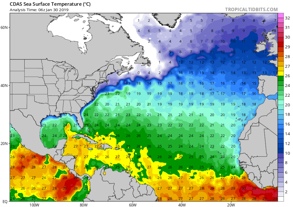
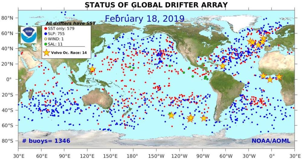volvo_globpop The best context for understanding decadal temperature changes comes from the world’s sea surface temperatures (SST), for several reasons:

The ocean covers 71% of the globe and drives average temperatures;
SSTs have a constant water content, (unlike air temperatures), so give a better reading of heat content variations;
A major El Nino was the dominant climate feature in recent years.

HadSST is generally regarded as the best of the global SST data sets, and so the temperature story here comes from that source, the latest version being HadSST3. More on what distinguishes HadSST3 from other SST products at the end.

The Current Context

The chart below shows SST monthly anomalies as reported in HadSST3 starting in 2015 through January 2019.

Hadsst012019

A global cooling pattern is seen clearly in the Tropics since its peak in 2016, joined by NH and SH cycling downward since 2016. 2018 started with slow warming after the low point of December 2017, led by steadily rising NH, which peaked in September and cooled the last 4 months. The Tropics rose steadily until November, and are now cooling as well. With little change in SH, the Global anomaly cooled further.

All regions are slightly warmer than 01/2015, but much cooler than 01/2016. The January Global anomaly is 0.2 lower than 2016; NH is 0.22 lower, SH is 0.16 lower and the Tropics are down 0.52 from 01/2016. The rise in the Tropics had suggested a possible El Nino, but is now cooling down.

Note that higher temps in 2015 and 2016 were first of all due to a sharp rise in Tropical SST, beginning in March 2015, peaking in January 2016, and steadily declining back below its beginning level. Secondly, the Northern Hemisphere added three bumps on the shoulders of Tropical warming, with peaks in August of each year. A fourth NH bump was lower and peaked in September 2018. Also, note that the global release of heat was not dramatic, due to the Southern Hemisphere offsetting the Northern one.

The annual SSTs for the last five years are as follows:

Annual SSTs	Global	NH	SH	Tropics
2014	0.477	0.617	0.335	0.451
2015	0.592	0.737	0.425	0.717
2016	0.613	0.746	0.486	0.708
2017	0.505	0.650	0.385	0.424
2018	0.480	0.620	0.362	0.369

2018 annual average SSTs across the regions are close to 2014, slightly higher in SH and much lower in the Tropics. The SST rise from the global ocean was remarkable, peaking in 2016, higher than 2011 by 0.32C.

A longer view of SSTs

The graph below is noisy, but the density is needed to see the seasonal patterns in the oceanic fluctuations. Previous posts focused on the rise and fall of the last El Nino starting in 2015. This post adds a longer view, encompassing the significant 1998 El Nino and since. The color schemes are retained for Global, Tropics, NH and SH anomalies. Despite the longer time frame, I have kept the monthly data (rather than yearly averages) because of interesting shifts between January and July.

Open image in new tab to enlarge.

1995 is a reasonable starting point prior to the first El Nino. The sharp Tropical rise peaking in 1998 is dominant in the record, starting Jan. ’97 to pull up SSTs uniformly before returning to the same level Jan. ’99. For the next 2 years, the Tropics stayed down, and the world’s oceans held steady around 0.2C above 1961 to 1990 average.

Then comes a steady rise over two years to a lesser peak Jan. 2003, but again uniformly pulling all oceans up around 0.4C. Something changes at this point, with more hemispheric divergence than before. Over the 4 years until Jan 2007, the Tropics go through ups and downs, NH a series of ups and SH mostly downs. As a result the Global average fluctuates around that same 0.4C, which also turns out to be the average for the entire record since 1995.

2007 stands out with a sharp drop in temperatures so that Jan.08 matches the low in Jan. ’99, but starting from a lower high. The oceans all decline as well, until temps build peaking in 2010.

Now again a different pattern appears. The Tropics cool sharply to Jan 11, then rise steadily for 4 years to Jan 15, at which point the most recent major El Nino takes off. But this time in contrast to ’97-’99, the Northern Hemisphere produces peaks every summer pulling up the Global average. In fact, these NH peaks appear every July starting in 2003, growing stronger to produce 3 massive highs in 2014, 15 and 16. NH July 2017 was only slightly lower, and a fifth NH peak still lower in Sept. 2018. Note also that starting in 2014 SH plays a moderating role, offsetting the NH warming pulses. (Note: these are high anomalies on top of the highest absolute temps in the NH.)

What to make of all this? The patterns suggest that in addition to El Ninos in the Pacific driving the Tropic SSTs, something else is going on in the NH. The obvious culprit is the North Atlantic, since I have seen this sort of pulsing before. After reading some papers by David Dilley, I confirmed his observation of Atlantic pulses into the Arctic every 8 to 10 years.

But the peaks coming nearly every summer in HadSST require a different picture. Let’s look at August, the hottest month in the North Atlantic from the Kaplan dataset.
AMO August 2018

The AMO Index is from from Kaplan SST v2, the unaltered and not detrended dataset. By definition, the data are monthly average SSTs interpolated to a 5×5 grid over the North Atlantic basically 0 to 70N. The graph shows warming began after 1992 up to 1998, with a series of matching years since. Because the N. Atlantic has partnered with the Pacific ENSO recently, let’s take a closer look at some AMO years in the last 2 decades.

amo-decade-122018

This graph shows monthly AMO temps for some important years. The Peak years were 1998, 2010 and 2016, with the latter emphasized as the most recent. The other years show lesser warming, with 2007 emphasized as the coolest in the last 20 years. Note the red 2018 line is at the bottom of all these tracks. Most recently December 2018 is 0.4C lower than December 2016, and is the coolest December since 2000.

Summary

The oceans are driving the warming this century. SSTs took a step up with the 1998 El Nino and have stayed there with help from the North Atlantic, and more recently the Pacific northern “Blob.” The ocean surfaces are releasing a lot of energy, warming the air, but eventually will have a cooling effect. The decline after 1937 was rapid by comparison, so one wonders: How long can the oceans keep this up? If the pattern of recent years continues, NH SST anomalies will likely cool in coming months. Once again, ENSO will probably determine the outcome.

Postscript:

In the most recent GWPF 2017 State of the Climate report, Dr. Humlum made this observation:

“It is instructive to consider the variation of the annual change rate of atmospheric CO2 together with the annual change rates for the global air temperature and global sea surface temperature (Figure 16). All three change rates clearly vary in concert, but with sea surface temperature rates leading the global temperature rates by a few months and atmospheric CO2 rates lagging 11–12 months behind the sea surface temperature rates.”

Footnote: Why Rely on HadSST3

HadSST3 is distinguished from other SST products because HadCRU (Hadley Climatic Research Unit) does not engage in SST interpolation, i.e. infilling estimated anomalies into grid cells lacking sufficient sampling in a given month. From reading the documentation and from queries to Met Office, this is their procedure.

HadSST3 imports data from gridcells containing ocean, excluding land cells. From past records, they have calculated daily and monthly average readings for each grid cell for the period 1961 to 1990. Those temperatures form the baseline from which anomalies are calculated.

In a given month, each gridcell with sufficient sampling is averaged for the month and then the baseline value for that cell and that month is subtracted, resulting in the monthly anomaly for that cell. All cells with monthly anomalies are averaged to produce global, hemispheric and tropical anomalies for the month, based on the cells in those locations. For example, Tropics averages include ocean grid cells lying between latitudes 20N and 20S.

Gridcells lacking sufficient sampling that month are left out of the averaging, and the uncertainty from such missing data is estimated. IMO that is more reasonable than inventing data to infill. And it seems that the Global Drifter Array displayed in the top image is providing more uniform coverage of the oceans than in the past.

USS Pearl Harbor deploys Global Drifter Buoys in Pacific Ocean

January Cooling by Land, A Surprise by Sea

Posted on February 9, 2019 by Ron Clutz

With apologies to Paul Revere, this post is on the lookout for cooler weather with an eye on both the Land and the Sea. UAH has updated their tlt (temperatures in lower troposphere) dataset for January. Previously I have done posts on their reading of ocean air temps as a prelude to updated records from HADSST3. This month I will add a separate graph of land air temps because the comparisons and contrasts are interesting as we contemplate possible cooling in coming months and years.

Presently sea surface temperatures (SST) are the best available indicator of heat content gained or lost from earth’s climate system. Enthalpy is the thermodynamic term for total heat content in a system, and humidity differences in air parcels affect enthalpy. Measuring water temperature directly avoids distorted impressions from air measurements. In addition, ocean covers 71% of the planet surface and thus dominates surface temperature estimates. Eventually we will likely have reliable means of recording water temperatures at depth.

Recently, Dr. Ole Humlum reported from his research that air temperatures lag 2-3 months behind changes in SST. He also observed that changes in CO2 atmospheric concentrations lag behind SST by 11-12 months. This latter point is addressed in a previous post Who to Blame for Rising CO2?

The January update to HadSST3 will appear later this month, but in the meantime we can look at lower troposphere temperatures (TLT) from UAHv6 which are already posted for January. The temperature record is derived from microwave sounding units (MSU) on board satellites like the one pictured above.

The UAH dataset includes temperature results for air above the oceans, and thus should be most comparable to the SSTs. There is the additional feature that ocean air temps avoid Urban Heat Islands (UHI). The graph below shows monthly anomalies for ocean temps since January 2015.

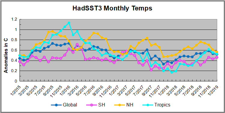
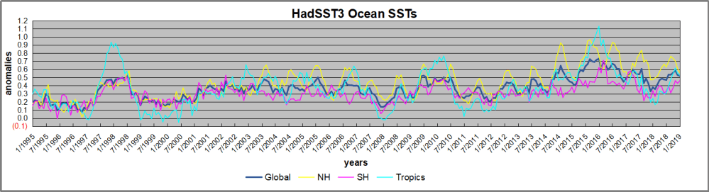
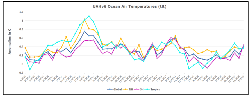UAH Oceans 201901 The anomalies over the entire ocean dropped to the same value, 0.12C in August (Tropics were 0.13C). Warming in previous months was erased, and September added very little warming back. In October and November NH and the Tropics rose, joined by SH. In December 2018 all regions cooled resulting in a global drop of nearly 0.1C. Now in January an upward jump in SH overcame slight cooling in NH and the Tropics, pulling up the Global anomaly as well. While the trajectory is not yet set, it is the highest ocean air January since 2016.

Land Air Temperatures Tracking Downward in Seesaw Pattern

We sometimes overlook that in climate temperature records, while the oceans are measured directly with SSTs, land temps are measured only indirectly. The land temperature records at surface stations record air temps at 2 meters above ground. UAH gives tlt anomalies for air over land separately from ocean air temps. The graph updated for January is below. UAH Land 201901

The greater volatility of the Land temperatures is evident, and also the dominance of NH, which has twice as much land area as SH. Note how global peaks mirror NH peaks. In December air over Tropics fell sharply, SH slightly, while the NH land surfaces rose, pulling up the Global anomaly for the month. In January both NH and SH cooled slightly, pulling the Global anomaly down despite some Tropical warming. Presently, air temps over land were the lowest January since 2014 both Globally and for the NH, despite warmer temps over SH and Tropical land areas.

Summary

TLTs include mixing above the oceans and probably some influence from nearby more volatile land temps. Clearly NH and Global land temps have been dropping in a seesaw pattern, now more than 1C lower than the peak in 2016. TLT measures started the recent cooling later than SSTs from HadSST3, but are now showing the same pattern. It seems obvious that despite the three El Ninos, their warming has not persisted, and without them it would probably have cooled since 1995. Of course, the future has not yet been written.

2019 Update: Climate Reductionism

Posted on February 6, 2019 by Ron Clutz

19170447-global_warming_1.530x298
With all the fuss about the “Green New Deal” and attempts to blame recent cold waves on rising CO2, it is wise to remember the logic of the alarmist argument. It boils down to two suppositions:

Rising atmospheric CO2 makes the planet warmer.

Rising emissions from humans burning fossil fuels makes atmospheric CO2 higher.

The second assertion is challenged in a post: Who to Blame for Rising CO2?

This post addresses the first claim. Remember also that all of the so-called “lines of evidence” for global warming do not distinguish between human and natural causes. Typically the evidence cited falls into these categories:

Global temperature rise
Warming oceans
Shrinking ice sheets
Glacial retreat
Decreased snow cover
Sea level rise
Declining Arctic sea ice
Extreme events

However, all of these are equivocal, involving signal and noise issues. Note also that all of them are alleged impacts from the first one. And in any case, the fact of any changes does not in itself prove human causation. That attribution rests solely on unvalidated climate models. Below is a discussion of the reductionist mental process by which climate complexity and natural forces are systematically excluded to reach the pre-determined conclusion.

Original Post: Climate Reductionism

Reductionists are those who take one theory or phenomenon to be reducible to some other theory or phenomenon. For example, a reductionist regarding mathematics might take any given mathematical theory to be reducible to logic or set theory. Or, a reductionist about biological entities like cells might take such entities to be reducible to collections of physico-chemical entities like atoms and molecules.
Definition from The Internet Encyclopedia of Philosophy

Some of you may have seen this recent article: Divided Colorado: A Sister And Brother Disagree On Climate Change

The reporter describes a familiar story to many of us. A single skeptic (the brother) is holding out against his sister and rest of the family who accept global warming/climate change. And of course, after putting some of their interchanges into the text, the reporter then sides against the brother by taking the word of a climate expert. From the article:

“CO2 absorbs infrared heat in certain wavelengths and those measurements were made first time — published — when Abraham Lincoln was president of the United States,” says Scott Denning, a professor of atmospheric science at Colorado State University. “Since that time, those measurements have been repeated by better and better instruments around the world.”

CO2, or carbon dioxide, has increased over time, scientists say, because of human activity. It’s a greenhouse gas that’s contributing to global warming.

“We know precisely how the molecule wiggles and waggles, and what the quantum interactions between the electrons are that cause everyone one of these little absorption lines,” he says. “And there’s just no wiggle room around it — CO2 absorbs heat, heat warms things up, so adding CO2 to the atmosphere will warm the climate.”

Denning says that most of the CO2 we see added to the atmosphere comes from humans — mostly through burning coal, oil and gas, which, as he puts it, is “indirectly caused by us.”

When looking at the scientific community, Denning says it’s united, as far as he knows.

earth-science-climatic-change-Climate-System-3-114-g001

A Case Study of Climate Reductionism

Denning’s comments, supported by several presentations at his website demonstrate how some scientists (all those known to Denning) engage in a classic form of reductionism.

The full complexity of earth’s climate includes many processes, some poorly understood, but known to have effects orders of magnitude greater than the potential of CO2 warming. The case for global warming alarm rests on simplifying away everything but the predetermined notion that humans are warming the planet. It goes like this:

Our Complex Climate

Earth’s climate is probably the most complicated natural phenomenon ever studied. Not only are there many processes, but they also interact and influence each other over various timescales, causing lagged effects and multiple cycling. This diagram illustrates some of the climate elements and interactions between them.

Flows and Feedbacks for Climate Models

The Many Climate Dimensions

Further, measuring changes in the climate goes far beyond temperature as a metric. Global climate indices, like the European dataset include 12 climate dimensions with 74 tracking measures. The set of climate dimensions include:

Sunshine
Pressure
Humidity
Cloudiness
Wind
Rain
Snow
Drought
Temperature
Heat
Cold

And in addition there are compound measures combining temperature and precipitation. While temperature is important, climate is much more than that. With this reduction, all other dimensions are swept aside, and climate change is simplified down to global warming as seen in temperature measurements.

Climate Thermodynamics: Weather is the Climate System at work.

Another distortion is the notion that weather is bad or good, depending on humans finding it favorable. In fact, all that we call weather are the ocean and atmosphere acting to resolve differences in temperatures, humidities and pressures. It is the natural result of a rotating, irregular planetary surface mostly covered with water and illuminated mostly at its equator.

The sun warms the surface, but the heat escapes very quickly by convection so the build-up of heat near the surface is limited. In an incompressible atmosphere, it would *all* escape, and you’d get no surface warming. But because air is compressible, and because gases warm up when they’re compressed and cool down when allowed to expand, air circulating vertically by convection will warm and cool at a certain rate due to the changing atmospheric pressure.

Climate science has been obsessed with only a part of the system, namely the atmosphere and radiation, in order to focus attention on the non-condensing IR active gases. The climate is framed as a 3D atmosphere above a 2D surface. That narrow scope leaves out the powerful non-radiative heat transfer mechanisms that dominate the lower troposphere, and the vast reservoir of thermal energy deep in the oceans.

As Dr. Robert E Stevenson writes, it could have been different:

“As an oceanographer, I’d been around the world, once or twice, and I was rather convinced that I knew the factors that influenced the Earth’s climate. The oceans, by virtue of their enormous density and heat-storage capacity, are the dominant influence on our climate. It is the heat budget and the energy that flows into and out of the oceans that basically determines the mean temperature of the global atmosphere. These interactions, plus evaporation, are quite capable of canceling the slight effect of man-produced CO2.”

The troposphere is dominated by powerful heat transfer mechanisms: conduction, convection and evaporation, as well as physical kinetic movements. All this is ignored in order to focus on radiative heat transfer, a bit player except at the top of the atmosphere.

There’s More than the Atmosphere

Once the world of climate is greatly reduced down to radiation of infrared frequencies, yet another set of blinders is applied. The most important source of radiation is of course the sun. Solar radiation in the short wave (SW) range is what we see and what heats up the earth’s surface, particularly the oceans. In addition solar radiation includes infrared, some absorbed in the atmosphere and some at the surface. The ocean is also a major source of heat into the atmosphere since its thermal capacity is 1000 times what the air can hold. The heat transfer from ocean to air is both by way of evaporation (latent heat) and also by direct contact at the sea surface (conduction).

Yet conventional climate science dismisses the sun as a climate factor saying that its climate input is unvarying. That ignores significant fluctuations in parts of the light range, for example ultraviolet, and also solar effects such as magnetic fields and cosmic rays. Also disregarded is solar energy varying due to cloud fluctuations. The ocean is also dismissed as a source of climate change despite obvious ocean warming and cooling cycles ranging from weeks to centuries. The problem is such oscillations are not well understood or predictable, so can not be easily modeled.

With the sun and the earth’s surface and ocean dismissed, the only consideration left is the atmosphere.

The Gorilla Greenhouse Gas

Thus climate has been reduced down to heat radiation passing through the atmosphere comprised of gases. One of the biggest reductions then comes from focusing on CO2 rather than H20. Of all the gases that are IR-active, water is the most prevalent and covers more of the spectrum.

The diagram below gives you the sense of proportion.

GHG blocks

The Role of CO2

We come now to the role of CO2 in “trapping heat” and making the world warmer. The theory is that CO2 acts like a blanket by absorbing and re-radiating heat that would otherwise escape into space. By delaying the cooling while solar energy comes in constantly, CO2 is presumed to cause a buildup of heat resulting in warmer temperatures.

How the Atmosphere Processes Heat

There are 3 ways that heat (Infrared or IR radiation) passes from the surface to space.

1) A small amount of the radiation leaves directly, because all gases in our air are transparent to IR of 10-14 microns (sometimes called the “atmospheric window.” This pathway moves at the speed of light, so no delay of cooling occurs.

2) Some radiation is absorbed and re-emitted by IR active gases up to the tropopause. Calculations of the free mean path for CO2 show that energy passes from surface to tropopause in less than 5 milliseconds. This is almost speed of light, so delay is negligible. H2O is so variable across the globe that its total effects are not measurable. In arid places, like deserts, we see that CO2 by itself does not prevent the loss of the day’s heat after sundown.

3) The bulk gases of the atmosphere, O2 and N2, are warmed by conduction and convection from the surface. They also gain energy by collisions with IR active gases, some of that IR coming from the surface, and some absorbed directly from the sun. Latent heat from water is also added to the bulk gases. O2 and N2 are slow to shed this heat, and indeed must pass it back to IR active gases at the top of the troposphere for radiation into space.

In a parcel of air each molecule of CO2 is surrounded by 2500 other molecules, mostly O2 and N2. In the lower atmosphere, the air is dense and CO2 molecules energized by IR lose it to surrounding gases, slightly warming the entire parcel. Higher in the atmosphere, the air is thinner, and CO2 molecules can emit IR into space. Surrounding gases resupply CO2 with the energy it lost, which leads to further heat loss into space.

This third pathway has a significant delay of cooling, and is the reason for our mild surface temperature, averaging about 15C. Yes, earth’s atmosphere produces a buildup of heat at the surface. The bulk gases, O2 and N2, trap heat near the surface, while IR active gases, mainly H20 and CO2, provide the radiative cooling at the top of the atmosphere. Near the top of the atmosphere you will find the -18C temperature.

Sources of CO2

Note the size of the human emissions next to the red arrow.

A final reduction comes down to how much of the CO2 in the atmosphere is there because of us. Alarmists/activists say any increase in CO2 is 100% man-made, and would be more were it not for natural CO2 sinks, namely the ocean and biosphere. The claim overlooks the fact that those sinks are also sources of CO2 and the flux from the land and sea is an order of magnitude higher than estimates of human emissions. In fact, our few Gigatons of carbon are lost within the error range of estimating natural emissions. Insects produce far more CO2 than humans do by all our activity, including domestic animals.

Why Climate Reductionism is Dangerous

Reducing the climate in this fashion reaches its logical conclusion in the Activist notion of the “450 Scenario.” Since Cancun, IPCC is asserting that global warming is capped at 2C by keeping CO2 concentration below 450 ppm. From Summary for Policymakers (SPM) AR5

Emissions scenarios leading to CO2-equivalent concentrations in 2100 of about 450 ppm or lower are likely to maintain warming below 2°C over the 21st century relative to pre-industrial levels. These scenarios are characterized by 40 to 70% global anthropogenic GHG emissions reductions by 2050 compared to 2010, and emissions levels near zero or below in 2100.

Thus is born the “450 Scenario” by which governments can be focused upon reducing human emissions without any reference to temperature measurements, which are troublesome and inconvenient. Almost everything in the climate world has been erased, and “Fighting Climate Change” is now code to mean accounting for fossil fuel emissions.

Conclusion

All propagandists begin with a kernel of truth, in this case the fact everything acting in the world has an effect on everything else. Edward Lorenz brought this insight to bear on the climate system in a ground breaking paper he presented in 1972 entitled: “Predictability: Does the Flap of a Butterfly’s Wings in Brazil Set Off a Tornado in Texas?” Everything does matter and has an effect. Obviously humans impact on the climate in places where we build cities and dams, clear forests and operate farms. And obviously we add some CO2 when we burn fossil fuels.

But it is wrong to ignore the major dominant climate realities in order to exaggerate a small peripheral factor for the sake of an agenda. It is wrong to claim that IR active gases somehow “trap” heat in the air when they immediately emit any energy absorbed, if not already lost colliding with another molecule. No, it is the bulk gases, N2 and O2, making up the mass of the atmosphere, together with the ocean delaying the cooling and giving us the mild and remarkably stable temperatures that we enjoy. And CO2 does its job by radiating the heat into space.

Since we do little to cause it, we can’t fix it by changing what we do. The climate will not stop changing because we put a price on carbon. And the sun will rise despite the cock going on strike to protest global warming.

Footnote: For a deeper understanding of the atmospheric physics relating to CO2 and climate, I have done a guide and synopsis of Murry Salby’s latest textbook on the subject: Fearless Physics from Dr. Salby

2019 AMOC Update: Oceans Moderate Climate Threat

Posted on February 1, 2019 by Ron Clutz

Update Feb.1, 2019 New Publication from M.S. Lozier et al.

f1.medium

The article is A sea change in our view of overturning in the subpolar North Atlantic which is reporting on the first 21 months of observations from the newly installed OSNAP array described in a previous post from a year ago (reprinted below). The article is paywalled, but the main findings are provided at a Science Daily article European waters drive ocean overturning, key for regulating climate. Excerpts in italics with my bolds.

Summary:
An international study reveals the Atlantic meridional overturning circulation, which helps regulate Earth’s climate, is highly variable and primarily driven by the conversion of warm, salty, shallow waters into colder, fresher, deep waters moving south through the Irminger and Iceland basins. This upends prevailing ideas and may help scientists better predict Arctic ice melt and future changes in the ocean’s ability to mitigate climate change by storing excess atmospheric carbon.

New research shows the Atlantic meridional overturning circulation, which regulates climate, is primarily driven by waters west of Europe.
Credit: Carolina Nobre, WHOI Media

In a departure from the prevailing scientific view, the study shows that most of the overturning and variability is occurring not in the Labrador Sea off Canada, as past modeling studies have suggested, but in regions between Greenland and Scotland. There, warm, salty, shallow waters carried northward from the tropics by currents and wind, sink and convert into colder, fresher, deep waters moving southward through the Irminger and Iceland basins.

Overturning variability in this eastern section of the ocean was seven times greater than in the Labrador Sea, and it accounted for 88 percent of the total variance documented across the entire North Atlantic over the 21-month study period.

“Overturning carries vast amounts of anthropogenic carbon deep into the ocean, helping to slow global warming,” said co-author Penny Holliday of the National Oceanography Center in Southampton, U.K. “The largest reservoir of this anthropogenic carbon is in the North Atlantic.”

“Overturning also transports tropical heat northward,” Holliday said, “meaning any changes to it could have an impact on glaciers and Arctic sea ice. Understanding what is happening, and what may happen in the years to come, is vital.”

MIT’s Carl Wunsch and other outside experts said the study was helpful, but pointed out that 21 months of study is not enough to know if this different location is temporary or permanent.

[Note: The comment about oceans taking up CO2 could be misleading. The ocean contains dissolved CO2 amounting to 50 times atmospheric CO2. Each year about 20% of all CO2 in the air goes into the ocean, replaced by outgassing CO2. The tiny fraction of atmospheric CO2 from humans is exchanged proportionately. Henry’s law applies to the water/air interface, so that a warmer ocean absorbs slightly less, and a colder ocean absorbs slightly more CO2. The exchange equilibrium is hardly disturbed by the little bit of human produced CO2. Thus the ocean serves as a massive buffer against human emissions.]

Previous Post: AMOC 2018: Not Showing Climate Threat

The RAPID moorings being deployed. Credit: National Oceanography Centre.

The AMOC is back in the news following a recent Ocean Sciences meeting. This update adds to the theme Oceans Make Climate. Background links are at the end, including one where chief alarmist M. Mann claims fossil fuel use will stop the ocean conveyor belt and bring a new ice age. Actual scientists are working away methodically on this part of the climate system, and are more level-headed. H/T GWPF for noticing the recent article in Science Ocean array alters view of Atlantic ‘conveyor belt’ By Katherine Kornei Feb. 17, 2018 . Excerpts with my bolds.

The powerful currents in the Atlantic, formally known as the Atlantic meridional overturning circulation (AMOC), are a major engine in Earth’s climate. The AMOC’s shallower limbs—which include the Gulf Stream—transport warm water from the tropics northward, warming Western Europe. In the north, the waters cool and sink, forming deeper limbs that transport the cold water back south—and sequester anthropogenic carbon in the process. This overturning is why the AMOC is sometimes called the Atlantic conveyor belt.

bams-d-16-0057.1-f1

Fig. 1. Schematic of the major warm (red to yellow) and cold (blue to purple) water pathways in the NASPG (North Atlantic subpolar gyre ) credit: H. Furey, Woods Hole Oceanographic Institution): Denmark Strait (DS), Faroe Bank Channel (FBC), East and West Greenland Currents (EGC and WGC, respectively), NAC, DSO, and ISO.

Last week, at the American Geophysical Union’s (AGU’s) Ocean Sciences meeting here, scientists presented the first data from an array of instruments moored in the subpolar North Atlantic. The observations reveal unexpected eddies and strong variability in the AMOC currents. They also show that the currents east of Greenland contribute the most to the total AMOC flow. Climate models, on the other hand, have emphasized the currents west of Greenland in the Labrador Sea. “We’re showing the shortcomings of climate models,” says Susan Lozier, a physical oceanographer at Duke University in Durham, North Carolina, who leads the $35-million, seven-nation project known as the Overturning in the Subpolar North Atlantic Program (OSNAP).

bams-d-16-0057.1-f2

Fig. 2. Schematic of the OSNAP array. The vertical black lines denote the OSNAP moorings with the red dots denoting instrumentation at depth. The thin gray lines indicate the glider survey. The red arrows show pathways for the warm and salty waters of subtropical origin; the light blue arrows show the pathways for the fresh and cold surface waters of polar origin; and the dark blue arrows show the pathways at depth for waters that originate in the high-latitude North Atlantic and Arctic.

The research and analysis is presented by Dr. Lozier et al. in this publication Overturning in the Subpolar North Atlantic Program: A New International Ocean Observing System Images above and text excerpted below with my bolds.

For decades oceanographers have assumed the AMOC to be highly susceptible to changes in the production of deep waters at high latitudes in the North Atlantic. A new ocean observing system is now in place that will test that assumption. Early results from the OSNAP observational program reveal the complexity of the velocity field across the section and the dramatic increase in convective activity during the 2014/15 winter. Early results from the gliders that survey the eastern portion of the OSNAP line have illustrated the importance of these measurements for estimating meridional heat fluxes and for studying the evolution of Subpolar Mode Waters. Finally, numerical modeling data have been used to demonstrate the efficacy of a proxy AMOC measure based on a broader set of observational data, and an adjoint modeling approach has shown that measurements in the OSNAP region will aid our mechanistic understanding of the low-frequency variability of the AMOC in the subtropical North Atlantic.

Fig. 7. (a) Winter [Dec–Mar (DJFM)] mean NAO index. Time series of temperature from the (b) K1 and (c) K9 moorings.

Finally, we note that while a primary motivation for studying AMOC variability comes from its potential impact on the climate system, as mentioned above, additional motivation for the measure of the heat, mass, and freshwater fluxes in the subpolar North Atlantic arises from their potential impact on marine biogeochemistry and the cryosphere. Thus, we hope that this observing system can serve the interests of the broader climate community.

Fig. 10. Linear sensitivity of the AMOC at (d),(e) 25°N and (b),(c) 50°N in Jan to surface heat flux anomalies per unit area. Positive sensitivity indicates that ocean cooling leads to an increased AMOC—e.g., in the upper panels, a unit increase in heat flux out of the ocean at a given location will change the AMOC at (d) 25°N or (e) 50°N 3 yr later by the amount shown in the color bar. The contour intervals are logarithmic. (a) The time series show linear sensitivity of the AMOC at 25°N (blue) and 50°N (green) to heat fluxes integrated over the subpolar gyre (black box with surface area of ∼6.7 × 10 m2) as a function of forcing lead time. The reader is referred to Pillar et al. (2016) for model details and to Heimbach et al. (2011) and Pillar et al. (2016) for a full description of the methodology and discussion relating to the dynamical interpretation of the sensitivity distributions.

In summary, while modeling studies have suggested a linkage between deep-water mass formation and AMOC variability, observations to date have been spatially or temporally compromised and therefore insufficient either to support or to rule out this connection.

Current observational efforts to assess AMOC variability in the North Atlantic.

The U.K.–U.S. Rapid Climate Change–Meridional Overturning Circulation and Heatflux Array (RAPID–MOCHA) program at 26°N successfully measures the AMOC in the subtropical North Atlantic via a transbasin observing system (Cunningham et al. 2007; Kanzow et al. 2007; McCarthy et al. 2015). While this array has fundamentally altered the community’s view of the AMOC, modeling studies over the past few years have suggested that AMOC fluctuations on interannual time scales are coherent only over limited meridional distances. In particular, a break point in coherence may occur at the subpolar–subtropical gyre boundary in the North Atlantic (Bingham et al. 2007; Baehr et al. 2009). Furthermore, a recent modeling study has suggested that the low-frequency variability of the RAPID–MOCHA appears to be an integrated response to buoyancy forcing over the subpolar gyre (Pillar et al. 2016). Thus, a measure of the overturning in the subpolar basin contemporaneous with a measure of the buoyancy forcing in that basin likely offers the best possibility of understanding the mechanisms that underpin AMOC variability. Finally, though it might be expected that the plethora of measurements from the North Atlantic would be sufficient to constrain a measure of the AMOC within the context of an ocean general circulation model, recent studies (Cunningham and Marsh 2010; Karspeck et al. 2015) reveal that there is currently no consensus on the strength or variability of the AMOC in assimilation/reanalysis products.

Atlantic Meridional Overturning Circulation (AMOC). Red colours indicate warm, shallow currents and blue colours indicate cold, deep return flows. Modified from Church, 2007, A change in circulation? Science, 317(5840), 908–909. doi:10.1126/science.1147796

In addition we have a recent report from the United Kingdom Marine Climate Change Impacts Partnership (MCCIP) lead author G.D. McCarthy Atlantic Meridional Overturning Circulation (AMOC) 2017.

Figure 1: Ten-day (colours) and three month (black) low-pass filtered timeseries of Florida Straits transport (blue), Ekman transport (green), upper mid-ocean transport (magenta), and overturning transport (red) for the period 2nd April 2004 to end- February 2017. Florida Straits transport is based on electromagnetic cable measurements; Ekman transport is based on ERA winds. The upper mid-ocean transport, based on the RAPID mooring data, is the vertical integral of the transport per unit depth down to the deepest northward velocity (~1100 m) on each day. Overturning transport is then the sum of the Florida Straits, Ekman, and upper mid-ocean transports and represents the maximum northward transport of upper-layer waters on each day. Positive transports correspond to northward flow.

The RAPID/MOCHA/WBTS array (hereinafter referred to as the RAPID array) has revolutionized basin scale oceanography by supplying continuous estimates of the meridional overturning transport (McCarthy et al., 2015), and the associated basin-wide transports of heat (Johns et al., 2011) and freshwater (McDonagh et al., 2015) at 10-day temporal resolution. These estimates have been used in a wide variety of studies characterizing temporal variability of the North Atlantic Ocean, for instance establishing a decline in the AMOC between 2004 and 2013.

Summary from RAPID data analysis

MCCIP reported in 2006 that:

a 30% decline in the AMOC has been observed since the early 1990s based on a limited number of observations. There is a lack of certainty and consensus concerning the trend;
most climate models anticipate some reduction in strength of the AMOC over the 21st century due to increased freshwater influence in high latitudes. The IPCC project a slowdown in the overturning circulation rather than a dramatic collapse.

And in 2017 that:
a substantial increase in the observations available to estimate the strength of the AMOC indicate, with greater certainty, a decline since the mid 2000s;
the AMOC is still expected to decline throughout the 21st century in response to a changing climate. If and when a collapse in the AMOC is possible is still open to debate, but it is not thought likely to happen this century.

And also that:

a high level of variability in the AMOC strength has been observed, and short term fluctuations have had unexpected impacts, including severe winters and abrupt sea-level rise;
recent changes in the AMOC may be driving the cooling of Atlantic ocean surface waters which could lead to drier summers in the UK.

Conclusions

The AMOC is key to maintaining the mild climate of the UK and Europe.
The AMOC is predicted to decline in the 21st century in response to a changing climate.
Past abrupt changes in the AMOC have had dramatic climate consequences.
There is growing evidence that the AMOC has been declining for at least a decade, pushing the Atlantic Multidecadal Variability into a cool phase.
Short term fluctuations in the AMOC have proved to have unexpected impacts, including being linked
with severe winters and abrupt sea-level rise.

Background:

Climate Pacemaker: The AMOC

Evidence is Mounting: Oceans Make Climate

Mann-made Global Cooling

2019 Update Scafetta vs. IPCC: Dueling Climate Theories

Posted on February 1, 2019 by Ron Clutz

In one corner, Darth Vader, the Prince of CO2, filling the air with the overwhelming sound of his poison breath. Opposing him, Luke Skywalker, a single skeptic armed only with facts and logic.

OK, that’s over the top, but it’s what came to mind while reading a new paper by Nicola Scafetta in which he goes up against the IPCC empire. And Star Wars came to mind since Scafetta’s theory involves astronomical cycles. The title below links to the text, which is well worth reading. Some excerpts follow in italics with my bolds. H/T GWPF

CMIP5 General Circulation Models versus a Semi-Empirical Model Based on Natural Oscillations

Updated 2019: Graph Comparing Scafetta Model with UAHv6

H/T Tallbloke for providing this image:

Green area is range of forecasts from CMIP5 models. Turquoise area is forecast from Scafetta astronomical climate model.

Scafetta comes out swinging: From the Abstract

Since 1850 the global surface temperature has warmed by about 0.9 oC. The CMIP5 computer climate models adopted by the IPCC have projected that the global surface temperature could rise by 2-5 oC from 2000 to 2100 for anthropogenic reasons. These projections are currently used to justify expensive mitigation policies to reduce the emission of anthropogenic greenhouse gases such as CO2.

However, recent scientific research has pointed out that the IPCC climate models fail to properly reconstruct the natural variability of the climate. Indeed, advanced techniques of analysis have revealed that the natural variability of the climate is made of several oscillations spanning from the decadal to the millennial scales (e.g. with periods of about 9.1, 10.4, 20, 60, 115, 1000 years and others). These oscillations likely have an astronomical origin.

In this short review I briefly summarize some of the main reasons why the AGWT should be questioned. In addition, I show that an alternative interpretation of climate change based on the evidences that a significant part of it is due to specific natural oscillations is possible. A modeling based on such interpretation agrees better with the climatic comprehensive picture deduced from the data.

The Missing Hot-Spot

It has been observed that for the last decades climate models predict a hot-spot, that is, a significant warming of a band of the upper troposphere 10 km over the tropics and the equator. The presence of this hot-spot is quite important because it would indicate that the water-vapor feedback to radiative forcing would be correctly reproduced by the models.

However, this predicted hot-spot has never been found in the tropospheric temperature records [20,21]. This could only be suggesting either that both the temperature records obtained with satellite measures and balloons have been poorly handled or that the models severely fail to properly simulate the water-vapor feedback. In the latter case, the flaw of the models would be fatal because the water-vapor feedback is the most important among the climate feedbacks.

Without a strong feedback response from water vapor the models would only predict a moderate climate sensitivity to radiative forcing of about 1.2 oC for CO2 doubling instead of about 3 oC. Figure 8 compares the observed temperature trend in the troposphere versus the climate model predictions: from Ref. [21]. The difference between the two record sets is evident.

Figure 8. Comparison between observed temperature trend in the troposphere (green-blue) versus the climate model predictions (red). From Ref. [21].

Observations Favor Scafetta’s Model Over GCM Models

I have proposed that the global surface temperature record could be reconstructed from the decadal to the millennial scale using a minimum of 6 harmonics at 9.1, 10.4, 20, 60, 115 and 983 years plus a anthropogenic and volcano contribution that can be evaluated from the CMIP5 GCM outputs reduced by half because, as discussed above, the real climate sensitivity to radiative forcing appears to be about half of what assumed by the current climate models. The figure highlights the better performance of the solar–astronomical semi-empirical model versus the CMIP5 models. This is particularly evident since 2000, as shown in the inserts.

Figure 12 [A] The four CMIP5 ensemble average projections versus the HadCRUT4 GST record (black). [B] The solar– astronomical semi-empirical model. From Ref. [4] Left axis shows temperature anomalies in degrees Celsius.

Forecast Validation

In 2011 I prepared a global surface temperature forecast based on a simplified climate model based on four natural oscillations (9.1, 10.4, 20 and 60 year) plus an estimate of a realistic anthropogenic contribution [25]: for example, see Refs. [33,34,35] referring to the 60-year cycle. Figure 13 compares my 2011 forecast (red curve) against the global surface temperature record I used in 2011 (HadCUT3, blue curve) and a modern global surface temperature record updated at June/2016 (RSS MSU record, black line, http://www.remss.com/measurements/upper-air-temperature).

The RSS MSU record, which is a global surface temperature estimate using satellite measurements, was linearly rescaled to fit the original HadCUT3 global surface temperature record for optimal comparison. Other global temperature reconstructions perform similarly. Note that the HadCUT3 has been dismissed in 2014. Figure 13 also shows in green a schematic representation of the IPCC GCMs prediction since 2000 [25].

Left axis shows temperature anomalies in degrees Celsius.

Figure 13. Comparison of the forecast (red-yellow curve) made in Scafetta (2011) [25] against (1) the temperature record used in 2011 (HadCRUT3, blue curve), (2) the IPCC climate model projections since 2000 (green area), (3) a recent global temperature record (RSS MSU record, black line, linearly re-scaled to match the HadCRUT3 from 1979 to 2014). The temperature record has followed Scafetta’s forecast better than the IPCC ones. In 2015-2016 there was a strong El-Nino Pacific Ocean natural warming that caused the observed temperature peak.

Summary

The considerations emerging from these findings yield to the conclusion that the IPCC climate models severely overestimate the anthropogenic climatic warming by about two times. I have finally proposed a semi-empirical climate model calibrated to reconstruct the natural climatic variability since Medieval times. I have shown that this model projects a very moderate warming until 2040 and a warming less than 2 oC from 2000 to 2100 using the same anthropogenic emission scenarios used by the CMIP5 models: see Figure 12.

This result suggests that climatic adaptation policies, which are less expensive than the mitigation ones, could be sufficient to address most of the consequences of a climatic change during the 21st century. Similarly, fossil fuels, which have contributed significantly to the development of our societies, can still be used to fulfill our energy necessities until equally efficient alternative energy sources could be determined and developed.

Scafetta Briefly Explains the Harmonic oscillation theory

“The theory is very simple in words. The solar system is characterized by a set of specific gravitational oscillations due to the fact that the planets are moving around the sun. Everything in the solar system tends to synchronize to these frequencies beginning with the sun itself. The oscillating sun then causes equivalent cycles in the climate system. Also the moon acts on the climate system with its own harmonics. In conclusion we have a climate system that is mostly made of a set of complex cycles that mirror astronomical cycles. Consequently it is possible to use these harmonics to both approximately hindcast and forecast the harmonic component of the climate, at least on a global scale. This theory is supported by strong empirical evidences using the available solar and climatic data.”

Update Nov. 20, 2017. Scafetta graph to June 2017

cooling-vs-warming-forecasts-scafetta-2017

From Natural climate variability, part 2: Interpretation of the post 2000
temperature standstill, Scafetta et al. 2017

Footnote: Scafetta is not alone. Dr. Norman Page has a new paper going into detail about forecasting climate by means of solar-astronomical patterns.

The coming cooling: Usefully accurate climate forecasting for policy makers

No, Cold Doesn’t Disprove Warming, Nothing Can

Posted on January 30, 2019 by Ron Clutz

That quote from Herodotus was put on the USPS building in Boston referring to postmen, ie postpersons today. (Are postpersons also postnormal? Just wondering). But I digress.

As bitter cold is hitting the US midwest, Trump chose to troll the warmists with a sympathetic tweet to those freezing their tails off. And now we get a deluge of articles declaring the title of this post. NOAA even drew a cartoon in response. Meanwhile some people bundled up and went to Niagara to witness the frozen falls.

In this context, the trusted couriers are the warmists swiftly making their rounds repeating their new message; “Heatwaves last summer prove global warming/climate change; Freezing cold this winter is also caused by warming.”

The evidence is in: Global warming is a religious belief, and adherents cannot be dissuaded by any fact, event or argument.

Footnote: USPS Suspended Service in 11 States Due to Record Low Temperatures.

N. Atlantic’s Cold Year

Posted on January 30, 2019 by Ron Clutz

RAPID Array measuring North Atlantic SSTs.

For the last few years, observers have been speculating about when the North Atlantic will start the next phase shift from warm to cold. Given the way 2018 went, this may be the onset. First some background.

Source: Energy and Education Canada

An example is this report in May 2015 The Atlantic is entering a cool phase that will change the world’s weather by Gerald McCarthy and Evan Haigh of the RAPID Atlantic monitoring project. Excerpts in italics with my bolds.

This is known as the Atlantic Multidecadal Oscillation (AMO), and the transition between its positive and negative phases can be very rapid. For example, Atlantic temperatures declined by 0.1ºC per decade from the 1940s to the 1970s. By comparison, global surface warming is estimated at 0.5ºC per century – a rate twice as slow.

In many parts of the world, the AMO has been linked with decade-long temperature and rainfall trends. Certainly – and perhaps obviously – the mean temperature of islands downwind of the Atlantic such as Britain and Ireland show almost exactly the same temperature fluctuations as the AMO.

Atlantic oscillations are associated with the frequency of hurricanes and droughts. When the AMO is in the warm phase, there are more hurricanes in the Atlantic and droughts in the US Midwest tend to be more frequent and prolonged. In the Pacific Northwest, a positive AMO leads to more rainfall.

A negative AMO (cooler ocean) is associated with reduced rainfall in the vulnerable Sahel region of Africa. The prolonged negative AMO was associated with the infamous Ethiopian famine in the mid-1980s. In the UK it tends to mean reduced summer rainfall – the mythical “barbeque summer”.Our results show that ocean circulation responds to the first mode of Atlantic atmospheric forcing, the North Atlantic Oscillation, through circulation changes between the subtropical and subpolar gyres – the intergyre region. This a major influence on the wind patterns and the heat transferred between the atmosphere and ocean.

The observations that we do have of the Atlantic overturning circulation over the past ten years show that it is declining. As a result, we expect the AMO is moving to a negative (colder surface waters) phase. This is consistent with observations of temperature in the North Atlantic.

Cold “blobs” in North Atlantic have been reported, but they are usually a winter phenomena. For example in April 2016, the sst anomalies looked like this

But by September, the picture changed to this

And we know from Kaplan AMO dataset, that 2016 summer SSTs were right up there with 1998 and 2010 as the highest recorded.

As the graph above suggests, this body of water is also important for tropical cyclones, since warmer water provides more energy. But those are annual averages, and I am interested in the summer pulses of warm water into the Arctic. As I have noted in my monthly HadSST3 reports, most summers since 2003 there have been warm pulses in the north atlantic.
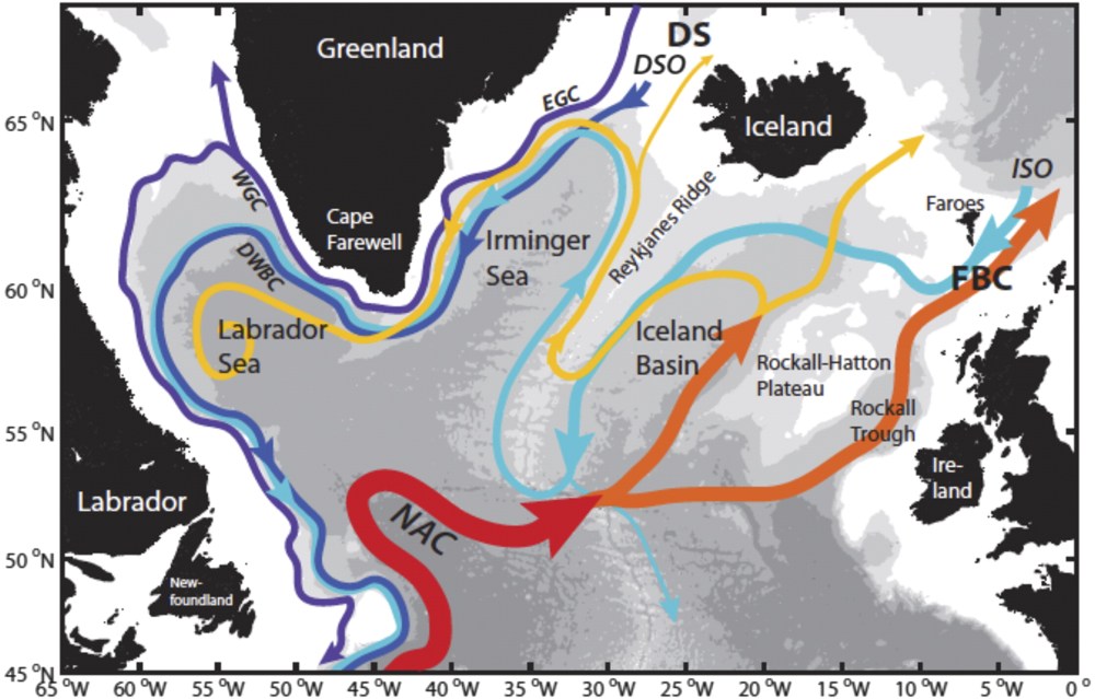
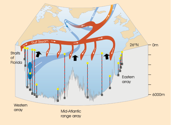
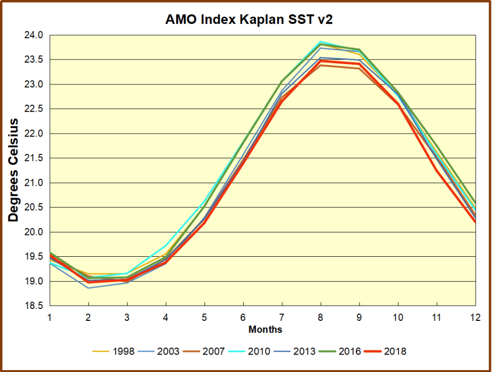
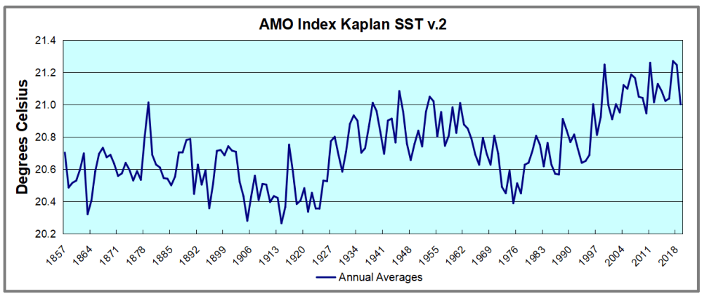
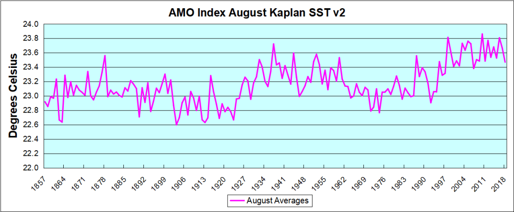
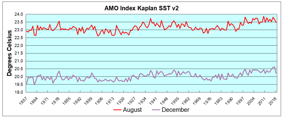amo december 2018 The AMO Index is from from Kaplan SST v2, the unaltered and not detrended dataset. By definition, the data are monthly average SSTs interpolated to a 5×5 grid over the North Atlantic basically 0 to 70N. The graph shows the warmest month August beginning to rise after 1993 up to 1998, with a series of matching years since. December 2016 set a record at 20.6C, but note the plunge down to 20.2C for December 2018, matching 2011 as the coldest years since 2000. Because McCarthy refers to hints of cooling to come in the N. Atlantic, let’s take a closer look at some AMO years in the last 2 decades.

amo decade 122018

With all the talk of AMOC slowing down and a phase shift in the North Atlantic, it seems the annual average for 2018 confirms that cooling has set in. Through December the momentum is certainly heading downward, despite the band of warming ocean that gave rise to European heat waves last summer.

amo annual122018

cdas-sflux_sst_atl_1

	Real World Energy Fl… on Refresher: GHG Theory and the…
	Greenland Ice Varies… on Greenland Ice Varies, Don’t Pa…
	IMF and World Bank M… on World of Hurt from Climate Pol…
	IMF and World Bank M… on Davos Ditches Climate, Focuses…
	Raymond Inauen on An Influencer’s Climate…