Reductionists are those who take one theory or phenomenon to be reducible to some other theory or phenomenon. For example, a reductionist regarding mathematics might take any given mathematical theory to be reducible to logic or set theory. Or, a reductionist about biological entities like cells might take such entities to be reducible to collections of physico-chemical entities like atoms and molecules.
Definition from The Internet Encyclopedia of Philosophy
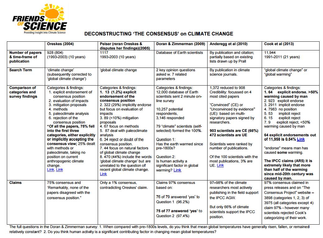
Some of you may have seen this recent article: Divided Colorado: A Sister And Brother Disagree On Climate Change
The reporter describes a familiar story to many of us. A single skeptic (the brother) is holding out against his sister and rest of the family who accept global warming/climate change. And of course, after putting some of their interchanges into the text, the reporter then sides against the brother by taking the word of a climate expert. From the article:
“CO2 absorbs infrared heat in certain wavelengths and those measurements were made first time — published — when Abraham Lincoln was president of the United States,” says Scott Denning, a professor of atmospheric science at Colorado State University. “Since that time, those measurements have been repeated by better and better instruments around the world.”
CO2, or carbon dioxide, has increased over time, scientists say, because of human activity. It’s a greenhouse gas that’s contributing to global warming.
“We know precisely how the molecule wiggles and waggles, and what the quantum interactions between the electrons are that cause everyone one of these little absorption lines,” he says. “And there’s just no wiggle room around it — CO2 absorbs heat, heat warms things up, so adding CO2 to the atmosphere will warm the climate.”
Denning says that most of the CO2 we see added to the atmosphere comes from humans — mostly through burning coal, oil and gas, which, as he puts it, is “indirectly caused by us.”
When looking at the scientific community, Denning says it’s united, as far as he knows.
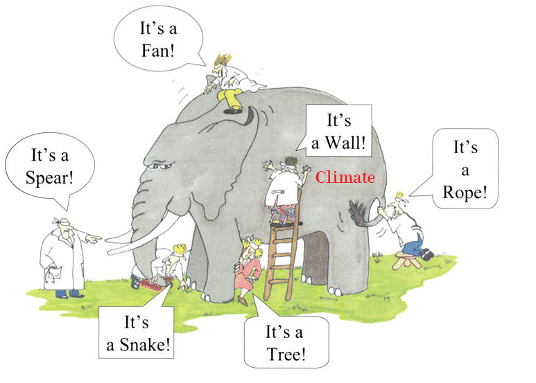
A Case Study of Climate Reductionism
Denning’s comments, supported by several presentations at his website demonstrate how some scientists (all those known to Denning) engage in a classic form of reductionism.
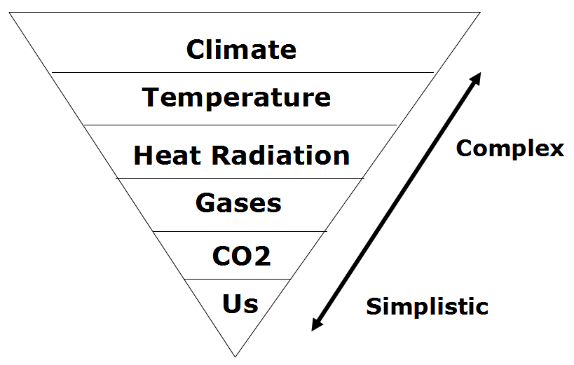
The full complexity of earth’s climate includes many processes, some poorly understood, but known to have effects orders of magnitude greater than the potential of CO2 warming. The case for global warming alarm rests on simplifying away everything but the predetermined notion that humans are warming the planet. It goes like this:
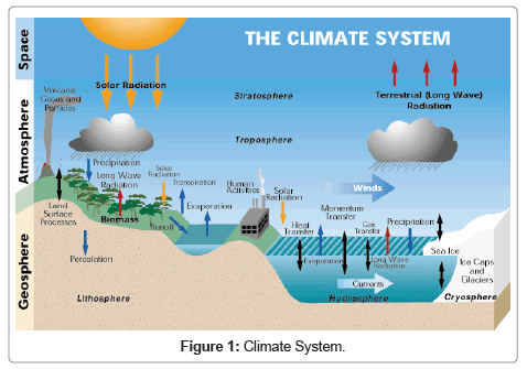
Our Complex Climate
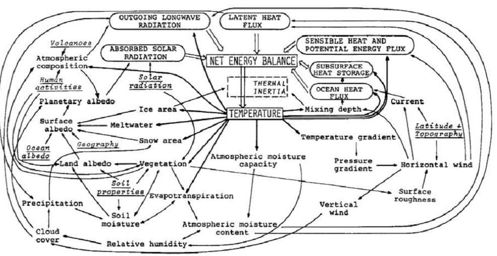
Earth’s climate is probably the most complicated natural phenomenon ever studied. Not only are there many processes, but they also interact and influence each other over various timescales, causing lagged effects and multiple cycling. This diagram illustrates some of the climate elements and interactions between them.

Flows and Feedbacks for Climate Models
The Many Climate Dimensions
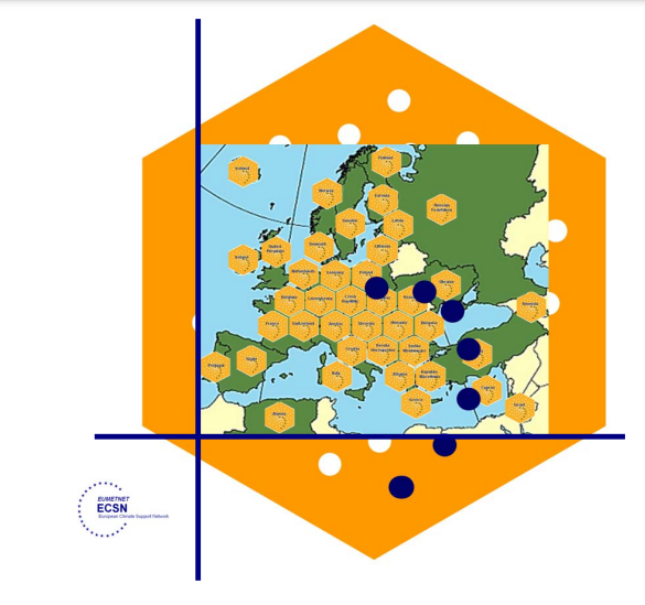
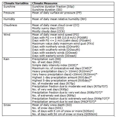
Further, measuring changes in the climate goes far beyond temperature as a metric. Global climate indices, like the European dataset include 12 climate dimensions with 74 tracking measures. The set of climate dimensions include:
- Sunshine
- Pressure
- Humidity
- Cloudiness
- Wind
- Rain
- Snow
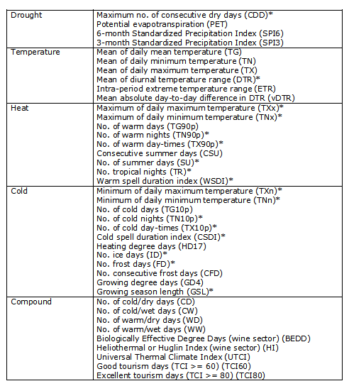
- Drought
- Temperature
- Heat
- Cold
And in addition there are compound measures combining temperature and precipitation. While temperature is important, climate is much more than that. With this reduction, all other dimensions are swept aside, and climate change is simplified down to global warming as seen in temperature measurements.
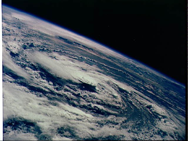
Climate Thermodynamics: Weather is the Climate System at work.
Another distortion is the notion that weather is bad or good, depending on humans finding it favorable. In fact, all that we call weather are the ocean and atmosphere acting to resolve differences in temperatures, humidities and pressures. It is the natural result of a rotating, irregular planetary surface mostly covered with water and illuminated mostly at its equator.
The sun warms the surface, but the heat escapes very quickly by convection so the build-up of heat near the surface is limited. In an incompressible atmosphere, it would *all* escape, and you’d get no surface warming. But because air is compressible, and because gases warm up when they’re compressed and cool down when allowed to expand, air circulating vertically by convection will warm and cool at a certain rate due to the changing atmospheric pressure.

Climate science has been obsessed with only a part of the system, namely the atmosphere and radiation, in order to focus attention on the non-condensing IR active gases. The climate is framed as a 3D atmosphere above a 2D surface. That narrow scope leaves out the powerful non-radiative heat transfer mechanisms that dominate the lower troposphere, and the vast reservoir of thermal energy deep in the oceans.
As Dr. Robert E Stevenson writes, it could have been different:
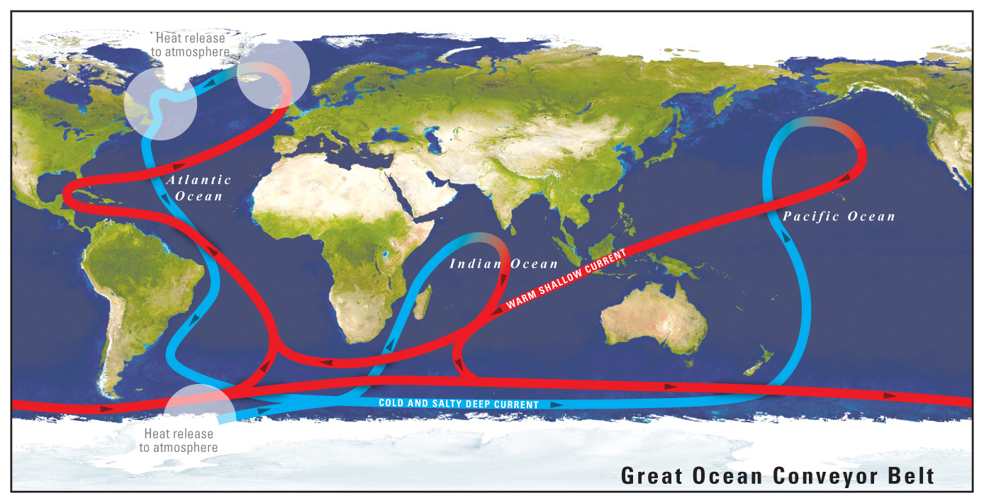
“As an oceanographer, I’d been around the world, once or twice, and I was rather convinced that I knew the factors that influenced the Earth’s climate. The oceans, by virtue of their enormous density and heat-storage capacity, are the dominant influence on our climate. It is the heat budget and the energy that flows into and out of the oceans that basically determines the mean temperature of the global atmosphere. These interactions, plus evaporation, are quite capable of canceling the slight effect of man-produced CO2.”
The troposphere is dominated by powerful heat transfer mechanisms: conduction, convection and evaporation, as well as physical kinetic movements. All this is ignored in order to focus on radiative heat transfer, a bit player except at the top of the atmosphere.

There’s More than the Atmosphere
Once the world of climate is greatly reduced down to radiation of infrared frequencies, yet another set of blinders is applied. The most important source of radiation is of course the sun. Solar radiation in the short wave (SW) range is what we see and what heats up the earth’s surface, particularly the oceans. In addition solar radiation includes infrared, some absorbed in the atmosphere and some at the surface. The ocean is also a major source of heat into the atmosphere since its thermal capacity is 1000 times what the air can hold. The heat transfer from ocean to air is both by way of evaporation (latent heat) and also by direct contact at the sea surface (conduction).
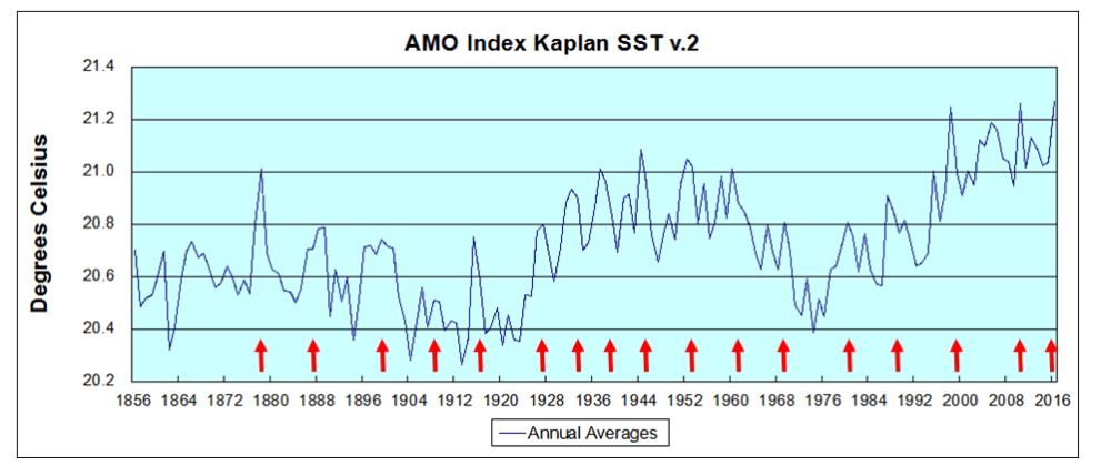
Yet conventional climate science dismisses the sun as a climate factor saying that its climate input is unvarying. That ignores significant fluctuations in parts of the light range, for example ultraviolet, and also solar effects such as magnetic fields and cosmic rays. Also disregarded is solar energy varying due to cloud fluctuations. The ocean is also dismissed as a source of climate change despite obvious ocean warming and cooling cycles ranging from weeks to centuries. The problem is such oscillations are not well understood or predictable, so can not be easily modeled.
With the sun and the earth’s surface and ocean dismissed, the only consideration left is the atmosphere.
The Gorilla Greenhouse Gas
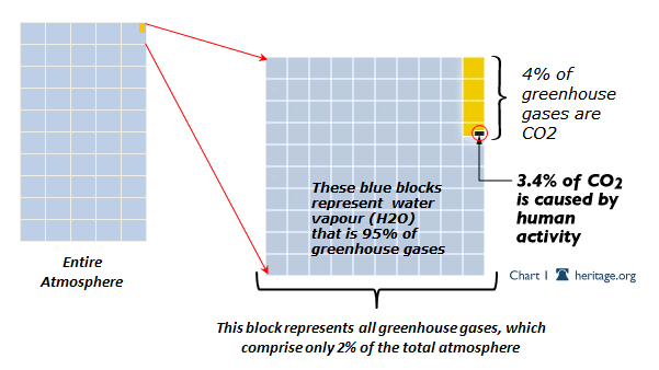
Thus climate has been reduced down to heat radiation passing through the atmosphere comprised of gases. One of the biggest reductions then comes from focusing on CO2 rather than H20. Of all the gases that are IR-active, water is the most prevalent and covers more of the spectrum.
The diagram below gives you the sense of proportion.
The Role of CO2
We come now to the role of CO2 in “trapping heat” and making the world warmer. The theory is that CO2 acts like a blanket by absorbing and re-radiating heat that would otherwise escape into space. By delaying the cooling while solar energy comes in constantly, CO2 is presumed to cause a buildup of heat resulting in warmer temperatures.
How the Atmosphere Processes Heat
There are 3 ways that heat (Infrared or IR radiation) passes from the surface to space.
1) A small amount of the radiation leaves directly, because all gases in our air are transparent to IR of 10-14 microns (sometimes called the “atmospheric window.” This pathway moves at the speed of light, so no delay of cooling occurs.
2) Some radiation is absorbed and re-emitted by IR active gases up to the tropopause. Calculations of the free mean path for CO2 show that energy passes from surface to tropopause in less than 5 milliseconds. This is almost speed of light, so delay is negligible. H2O is so variable across the globe that its total effects are not measurable. In arid places, like deserts, we see that CO2 by itself does not prevent the loss of the day’s heat after sundown.
3) The bulk gases of the atmosphere, O2 and N2, are warmed by conduction and convection from the surface. They also gain energy by collisions with IR active gases, some of that IR coming from the surface, and some absorbed directly from the sun. Latent heat from water is also added to the bulk gases. O2 and N2 are slow to shed this heat, and indeed must pass it back to IR active gases at the top of the troposphere for radiation into space.
In a parcel of air each molecule of CO2 is surrounded by 2500 other molecules, mostly O2 and N2. In the lower atmosphere, the air is dense and CO2 molecules energized by IR lose it to surrounding gases, slightly warming the entire parcel. Higher in the atmosphere, the air is thinner, and CO2 molecules can emit IR into space. Surrounding gases resupply CO2 with the energy it lost, which leads to further heat loss into space.
This third pathway has a significant delay of cooling, and is the reason for our mild surface temperature, averaging about 15C. Yes, earth’s atmosphere produces a buildup of heat at the surface. The bulk gases, O2 and N2, trap heat near the surface, while IR active gases, mainly H20 and CO2, provide the radiative cooling at the top of the atmosphere. Near the top of the atmosphere you will find the -18C temperature.
Sources of CO2
Note the size of the human emissions next to the red arrow.
A final reduction comes down to how much of the CO2 in the atmosphere is there because of us. Alarmists/activists say any increase in CO2 is 100% man-made, and would be more were it not for natural CO2 sinks, namely the ocean and biosphere. The claim overlooks the fact that those sinks are also sources of CO2 and the flux from the land and sea is an order of magnitude higher than estimates of human emissions. In fact, our few Gigatons of carbon are lost within the error range of estimating natural emissions. Insects produce far more CO2 than humans do by all our activity, including domestic animals.
Why Climate Reductionism is Dangerous
Reducing the climate in this fashion reaches its logical conclusion in the Activist notion of the “450 Scenario.” Since Cancun, IPCC is asserting that global warming is capped at 2C by keeping CO2 concentration below 450 ppm. From Summary for Policymakers (SPM) AR5
Emissions scenarios leading to CO2-equivalent concentrations in 2100 of about 450 ppm or lower are likely to maintain warming below 2°C over the 21st century relative to pre-industrial levels. These scenarios are characterized by 40 to 70% global anthropogenic GHG emissions reductions by 2050 compared to 2010, and emissions levels near zero or below in 2100.
Thus is born the “450 Scenario” by which governments can be focused upon reducing human emissions without any reference to temperature measurements, which are troublesome and inconvenient. Almost everything in the climate world has been erased, and “Fighting Climate Change” is now code to mean accounting for fossil fuel emissions.
Conclusion
All propagandists begin with a kernel of truth, in this case the fact everything acting in the world has an effect on everything else. Edward Lorenz brought this insight to bear on the climate system in a ground breaking paper he presented in 1972 entitled: “Predictability: Does the Flap of a Butterfly’s Wings in Brazil Set Off a Tornado in Texas?” Everything does matter and has an effect. Obviously humans impact on the climate in places where we build cities and dams, clear forests and operate farms. And obviously we add some CO2 when we burn fossil fuels.
But it is wrong to ignore the major dominant climate realities in order to exaggerate a small peripheral factor for the sake of an agenda. It is wrong to claim that IR active gases somehow “trap” heat in the air when they immediately emit any energy absorbed, if not already lost colliding with another molecule. No, it is the bulk gases, N2 and O2, making up the mass of the atmosphere, together with the ocean delaying the cooling and giving us the mild and remarkably stable temperatures that we enjoy. And CO2 does its job by radiating the heat into space.
Since we do little to cause it, we can’t fix it by changing what we do. The climate will not stop changing because we put a price on carbon. And the sun will rise despite the cock going on strike to protest global warming.
Footnote: For a deeper understanding of the atmospheric physics relating to CO2 and climate, I have done a guide and synopsis of Murry Salby’s latest textbook on the subject: Fearless Physics from Dr. Salby


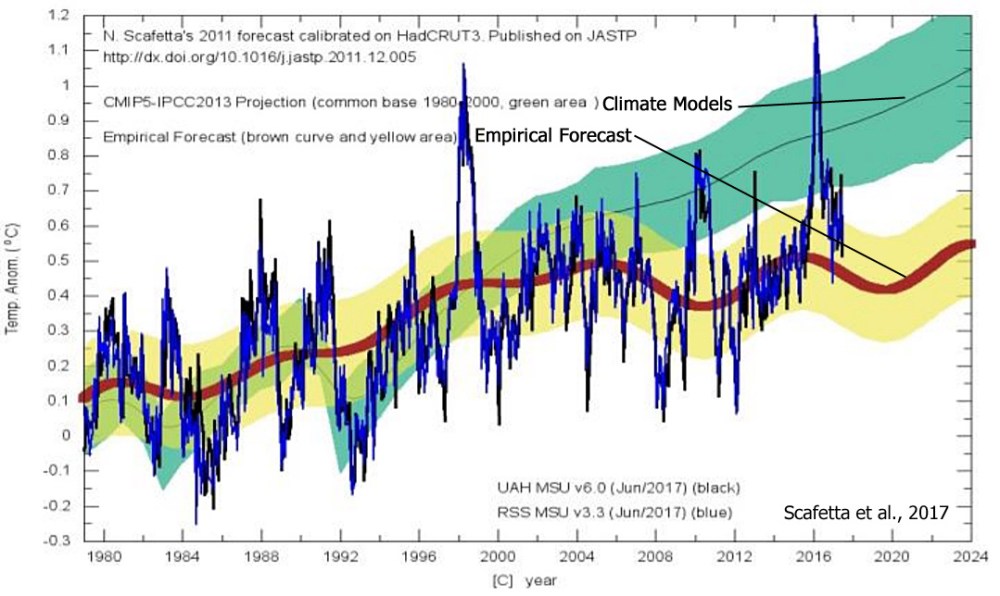
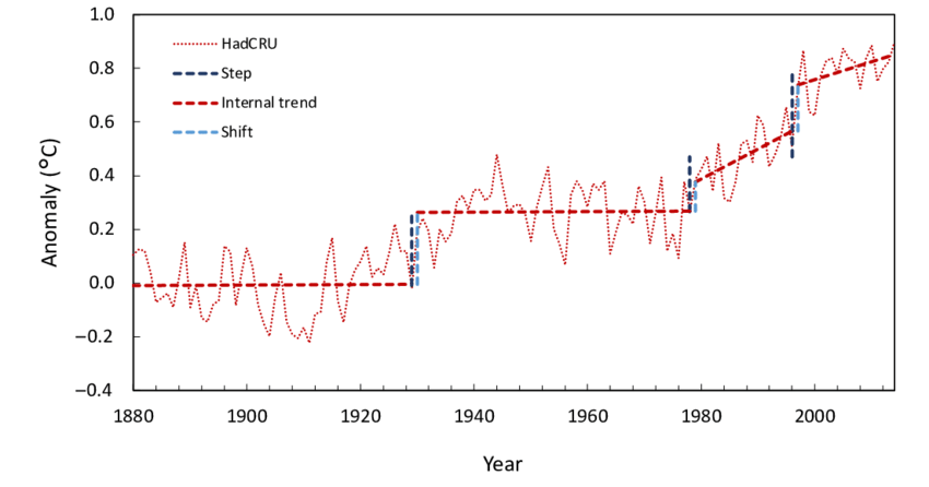
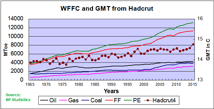
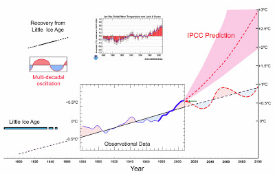 Note that the hypothesis is virtually the same, except for the leap of faith to attribute the secular background rise to CO2, rather than to a steady recovery from the Little Ice Age (LIA). Finally climate modelers are admitting that natural variability is strong enough to offset warming from any other means. And by extension the rise in temperatures late last century was due in large measure to a warming natural phase.