David Stockman: Resist the GreenMageddon, Part 1
This post is the first of five to alert readers to a compilation of the scientific case against the claims of IPCC supporters and anti-fossil fuel activists. David Stockman provides the evidence and the arguments against the IPCC policy framework in a series of five essays published at International Man under the title The GreenMageddon and What It Means for You. I will state the five themes he develops in his essays, along with some excerpts and images to illustrate the main points. Here is an overview followed by the first theme.

Overview

With COP26 now underway, it’s not too soon to start clanging the alarm bells—not about climate catastrophe, of course, but about the stupidest act of the assembled nations since Versailles, when the vindictive WWI victors laid the groundwork for the catastrophes of depression, WWII, the Holocaust, Soviet tyranny, the Cold War and Washington’s destructive global hegemony, all of which followed hard upon the next.

Politicians and their allies in the mainstream media, think tanks, lobbies and Big Business (with its cowardly sleep-walking leaders) are fixing to do nothing less than destroy the prosperity of the world and send global life careening into a modern economic Dark Ages.

And worse still, it’s being done in the service of a bogus climate crisis narrative that is thoroughly anti-science and wholly inconsistent with the actual climate and CO2 history of the planet.

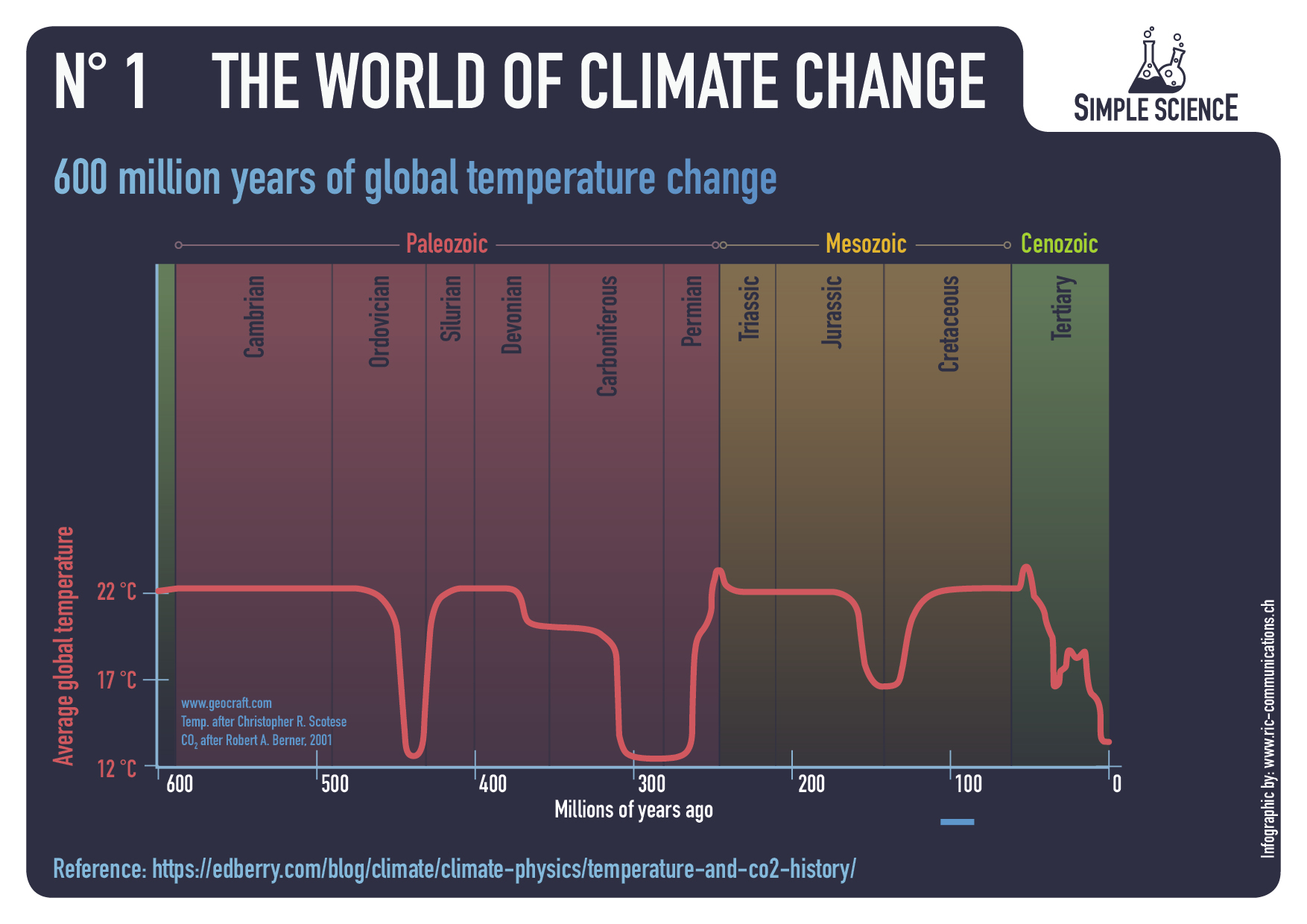
1. During the past 600 million years, the earth has rarely been as cool as at present, and almost never has it had as low CO2 concentrations as the 420 ppm level that today’s climate howlers decry.

In fact, according to the careful reconstructions of actual earth scientists who have studied ocean sediments, ice cores and the like, there have been only two periods encompassing about 75 million years (13% of that immensely long 600 million year stretch of time) where temperatures and CO2 concentrations were as low as it present. These were the Late Carboniferous/Early Permian time from 315 to 270 million years ago and the Quaternary Period, which hosted modern man 2.6 million years ago.  You might say, therefore, that the possibility of a warmer, CO2-richer environment is a case of planetary “been there, done that”.

And it is most certainly not a reason to wantonly dismantle and destroy the intricate, low-cost energy system that is the root source of today’s unprecedented prosperity and human escape from poverty and want.

But that’s hardly the half of it. What actually lies smack in the center of our warmer past is a 220-million-year interval from 250 million years ago through the re-icing of Antarctica about 33 million years ago that was mainly ice-free.

As shown by the blue line in the chart below, during most of that period (highlighted in the brown panels), temperatures were up to 12C higher than at present, and Mother Earth paid no mind to the fact that she lacked polar ice caps or suitable habitats for yet un-evolved polar bears.

Global Temperature And Atmospheric CO2 Over Geologic Time

Moreover, the science behind this isn’t a matter of academic armchair speculation for the simple reason that it has been powerfully validated in the commercial marketplace. That is, trillions of dollars have been deployed in the last century in the search for hydrocarbons, based on immensely complicated petroleum engineering research, theory and geologic models. Oil drillers weren’t throwing darts at a wildcatter’s wall but were coincidentally proving these “facts” of climate history are correct, given that they led to the discovery and extraction of several trillions of BOEs (barrels of oil equivalent).

Consequently, it is solidly estimated by industry experts that today’s petroleum deposits were roughly formed as follows:

    • About 70% during the Mesozoic age (brown panels, 252 to 66 million years ago) which was marked by a tropical climate, with large amounts of plankton in the oceans;
    • 20% was formed in the dryer, colder Cenozoic age (last 65 million years);
    • 10% were formed in the earlier warmer Paleozoic age (541 to 252 million years ago).

Indeed, at the end of the day, petroleum engineering is rooted in climate science because it was climate itself that produced those economically valuable deposits.

And a pretty awesome science it is. After all, billions of dollars have been pushed down the wellbores in up to two miles of ocean waters and 40,000 feet below the surface in what amounts to an amazingly calibrated and targeted search for oil-bearing needles in a geologic haystack.

Yet during the Cretaceous, CO2 levels actually went down while temperatures were rising sharply. That’s the very opposite of the Climate Alarmists’ core claim that it is rising CO2 concentrations which are currently forcing global temperatures higher.

Moreover, we are not talking about a marginal reduction in CO2 concentrations in the atmosphere. Levels actually dropped sharply from about 2,000 ppm to 900 ppm during that 80 million year stretch. This was all good for hydrocarbon formation and today’s endowment of nature’s stored work, but it was also something more.

To wit, it was yet another proof that planetary climate dynamics are far more complicated and ridden with crosscurrents than the simple-minded doom loops now being used to model future climate states from the current far lower temperature and CO2 levels.

It is surely one of the great ironies of our times that today’s fanatical crusades against fossil fuels are being carried out with not even a nod to the geologic history that contradicts the entire “warming” and CO2 concentration hysteria and made present energy consumption levels and efficiencies possible.

That is to say, the big, warm and wet one (the Mesozoic) got us here.

True global warming is not the current and future folly of mankind; it is the historical enabler of present-day economic blessings. Yet, here we are on the eve of COP26, manically focused on reducing emissions to the levels required to keep global temperatures from rising more than 1.5 degrees Celsius from preindustrial levels.

If your brain is not addled by the climate change narrative, the very term rings a resoundingly loud bell. That’s because there have been on the order of 20 distinct “ice ages” and interglacial warming periods during the Pleistocene, the latest of which ended about 18,000 years ago and from which we have been digging out ever since.

In contrast to today’s climate models, Mother Nature clearly did not go off the rails in some kind of linear doomsday loop of ever-increasing temperatures and without any hectoring from Greta, either. Actually, Greenland got all frozen up and thawed several more times thereafter.

Needless to say, the Holocene Optimum 8,000 years ago is not the “preindustrial” baseline from which the Climate Howlers are pointing their phony hockey sticks. In fact, other studies show that, even in the Arctic, it was no picnic time for the polar bears. Among 140 sites across the western Arctic, there is clear evidence for conditions that were warmer than now at 120 sites. At 16 sites for which quantitative estimates have been obtained, local temperatures were on average 1.6 °C higher during the optimum than they are today.

Say what? Isn’t that the same +1.6 degrees C above current levels that the COP26 folks are threatening to turn off the lights of prosperity to prevent?

In any event, what did happen was far more beneficent. To wit, the warmer and wetter Holocene Optimum and its aftermath gave rise to the great river civilizations 5,000 years ago, including the Yellow River in China, the Indus River in the Indian subcontinent, the Tigris-Euphrates and the Nile River civilizations among the most notable.

Stated differently, that +1.6 degrees C was reflective of the climate-based catalyzing forces that actually made today’s world possible. From the abundances of the river civilizations, there followed the long march of agriculture and the economic surpluses and abundance that enabled cities, literacy, trade and specialization, advancement of tools and technology and modern industry—the latter being the ultimate human escape from a life based on the back muscles of man and his domesticated animals alone.

As it happens, when one of the previous “preindustrial” warming eras (the Roman Warming) was coming to an end in the late 4th century AD, St. Jerome admonished the faithful “never look a gift horse in the mouth.”

Yet that’s exactly what the assembled nations will be doing at COP26.


We Are CO2

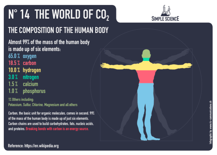
Raymond has published a new slide on the World of CO2, shown above.  Carbon is an essential part of every human body, as explained in the accompanying text:

The organic molecules of the human body consist of carbon chains that are used to build carbohydrates, fats, nucleic acids and proteins. The breakdown of carbon compounds is the source of energy we need to live. The air we breathe provides the oxygen needed to break the carbon bond, which then produces CO2, that we exhale.

The set of 14 infographics can be accessed at The World of CO2 – RIC Communications

Infographics can be helpful, in making things simple to understand. CO2 is a complex topic with a lot of information and statistics. These simple step by step charts should help to give you an idea of CO2’s importance. Without CO2, plants wouldn’t be able to live on this planet. Just remember, that if CO2 falls below 150 ppm, all plant life would cease to exist.

– N° 1 Earth’s atmospheric composition
– N° 2 Natural sources of CO2 emissions
– N° 3 Global anthropogenic CO2 emissions
– N° 4 CO2 – Carbon dioxide molecule
– N° 5 The global carbon cycle
– N° 6 Carbon and plant respiration
– N° 7 Plant categories and abundance (C3, C4 & CAM Plants)
– N° 8 Photosynthesis, the C3 vs C4 gap
– N° 9 Plant respiration and CO2
– N° 10 The logarithmic temperature rise of higher CO2 levels.
– N° 11 Earth’s atmospheric composition in relationship to CO2
– N° 12 Human respiration and CO2 concentrations.
– N° 13 600 million years of temperature change and atmospheric CO2

There is also a high quality introductory video:

Raymond has also produced a second series of Simple Science graphics on the theme The World of Climate Change.

Infographics can be helpful, in making things simple to understand. Climate change is a complex topic with a lot of information and statistics. These simple step by step charts are here to better understand what is occurring naturally and what could be caused by humans. What is cause for alarm and what isn’t cause for alarmism if at all. Only through learning is it possible to get the big picture so as to make the right decisions for the future.

– N° 1 600 million years of global temperature change
– N° 2 Earth‘s temperature record for the last 400,000 years
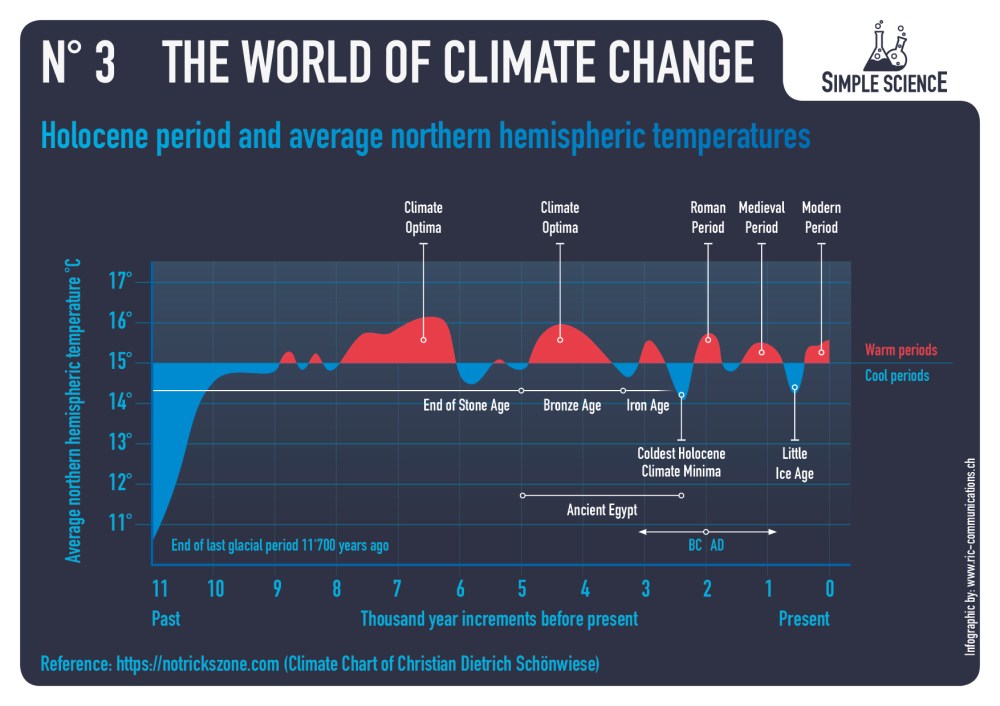
– N° 3 Holocene period and average northern hemispheric temperatures
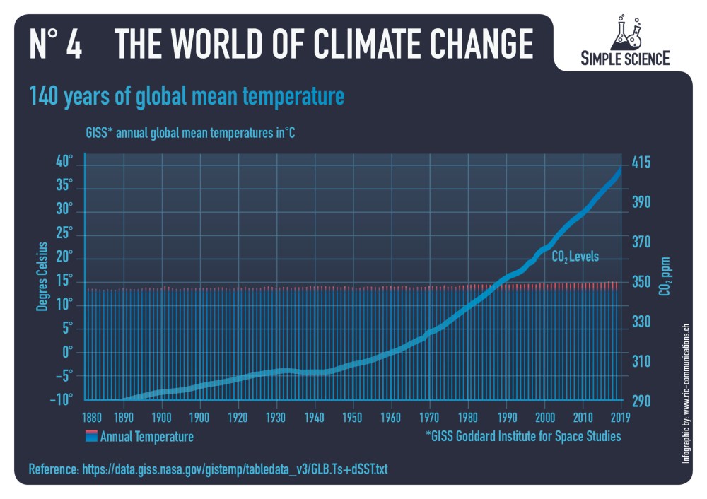
– N° 4 140 years of global mean temperature
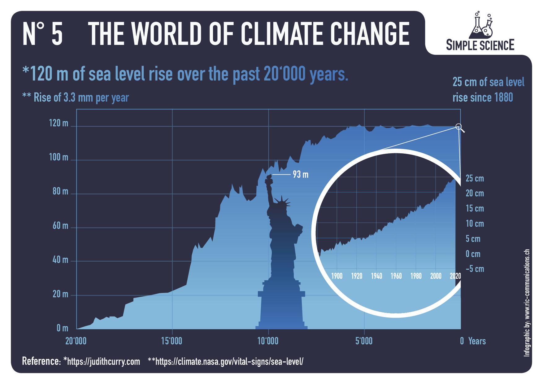
– N° 5 120 m of sea level rise over the past 20‘000 years
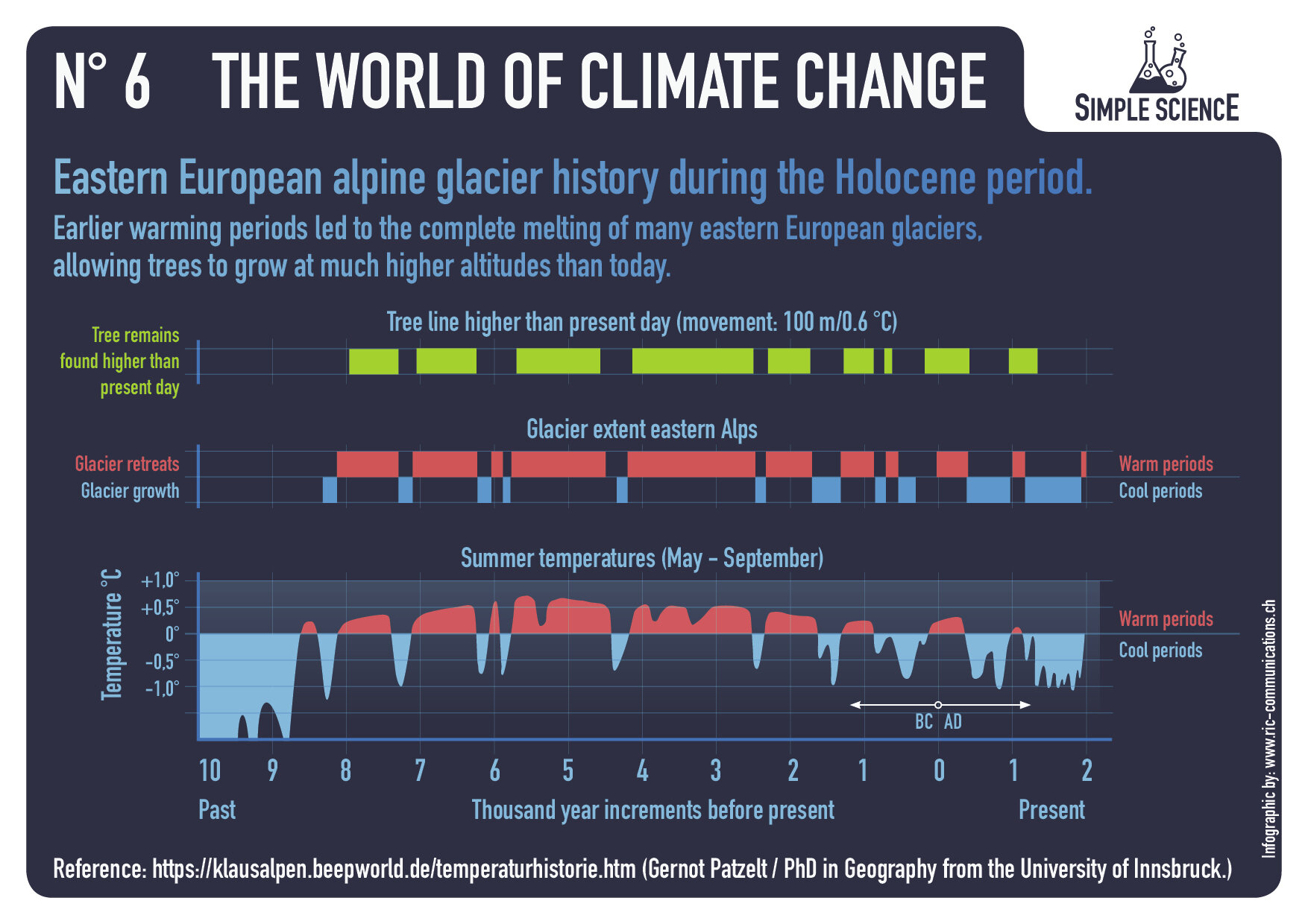
– N° 6 Eastern European alpine glacier history during the Holocene period.

For example:

How Do We Know Humans Cause Climate Change?

Peter J. Wallison and Benjamin Zycher examine the evidence in their Law & Liberty article What We Really Know About Climate Change.  Excerpts in italics with my bolds and added images.

The assumption that humans are the single most significant cause of climate change is unsupported by the available science.

The sixth Assessment Report (AR6) of the Intergovernmental Panel on Climate Change (IPCC) continues a long history of alarmist predictions with the deeply dubious statement that human-caused climate change has now become “irreversible.” President Biden and many others have called climate change an “existential threat” to humanity; and Biden claimed in his inaugural address to have heard from the Earth itself “a cry for survival.”

Hurricane Ida also has brought new claims about the dangers of climate change, but those assertions are inconsistent with the satellite record on tropical cyclones, which shows no trend since the early 1970s.

Yet the headline on the front page of the New York Times of August 12, 2021 was: “Greek Island Burns in a Sign of Crises to Come.” The accompanying article, continuing the multi-year effort of that newspaper to spread fears about climate change unsupported by evidence, argued that this was “another inevitable episode of Europe’s extreme weather [caused] by the man-made climate change that scientists have now concluded is irreversible.”

Almost every word in that sentence is either false or seriously misleading, continuing a multi-decade campaign of apocalyptic warnings about the effects of greenhouse gas emissions. Data on centuries and millennia of climate phenomena, constructed by scientists over many years around the world, show that the severe weather that the Times attributes to “man-made climate change” is consistent with the normal weather patterns and variability displayed in both the formal records and such proxy data as ice cores. In fact, there is little evidence that “extreme weather” events have become more frequent since 1850, the approximate end of the little ice age.

Increasing atmospheric concentrations of greenhouse gases have yielded detectable effects, but “scientists” in general have not, as the Times falsely stated, concluded that “extreme weather” is now “irreversible.” The statement itself comes from the “Summary for Policymakers” published as part of the most recent IPCC study of climate change; it is deeply problematic given the analyses and data provided in the scientific chapter (“The Physical Science Basis”) of the report to which the Times referred. Scientists disagree sharply about the significance of climate change and the analytic tools used to evaluate it, let alone whether it is “irreversible.”

There has been no upward trend in the number of “hot” days between 1895 and 2017; 11 of the 12 years with the highest number of such days occurred before 1960. Since 2005, NOAA has maintained the U.S. Climate Reference Network, comprising 114 meticulously maintained temperature stations spaced more or less uniformly across the lower 48 states, along with 21 stations in Alaska and two stations in Hawaii. They are placed to avoid heat-island effects and other such distortions as much as possible. The reported data show no increase in average temperatures over the available 2005-2020 period. In addition, a recent reconstruction of global temperatures over the past 1 million years—created using data from ice-sheet formations—shows that there is nothing unusual about the current warm period.
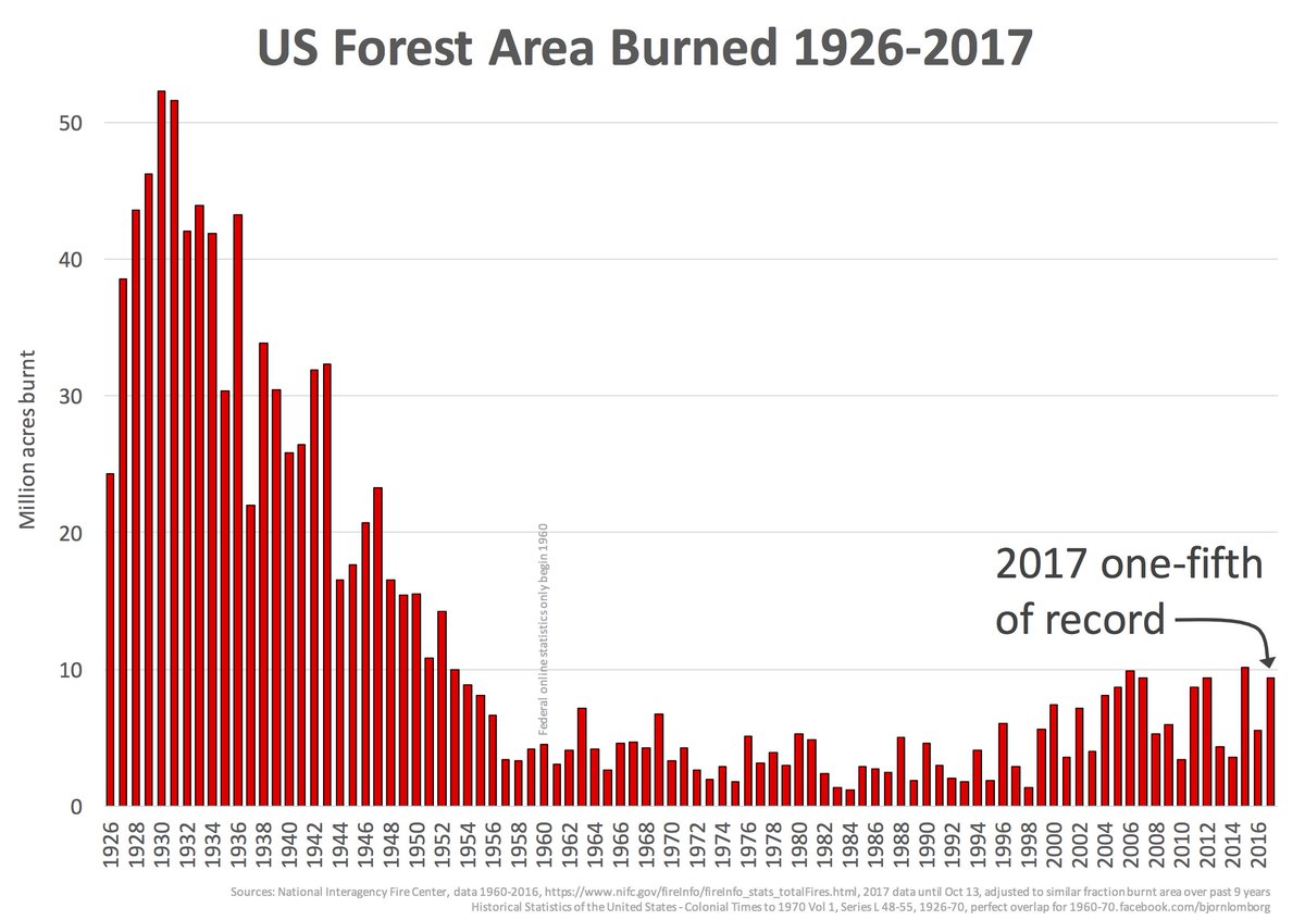
These alarmist predictions almost always are based upon climate models that have proven poor at reconstructing the past and ongoing temperature record. For example, the Times article implies that wildfires will increase in the future as the earth grows hotter. But there has been no trend in the number of U.S. wildfires in the 35 years since 1985, and global acreage burned has declined over past decades.

Unable to demonstrate that observed climate trends are due to human-caused (anthropogenic) climate change—or even that these events are particularly unusual or concerning—climate catastrophists will often turn to dire predictions about prospective climate phenomena. The problem with such predictions is that they are almost always generated by climate models driven by highly complex sets of assumptions about which there is significant dispute. It goes without saying that the predictions of models that cannot reconstruct what has happened in the past should not be given heavy weight in terms of predictions about the future, but that is exactly what many analysts are doing.

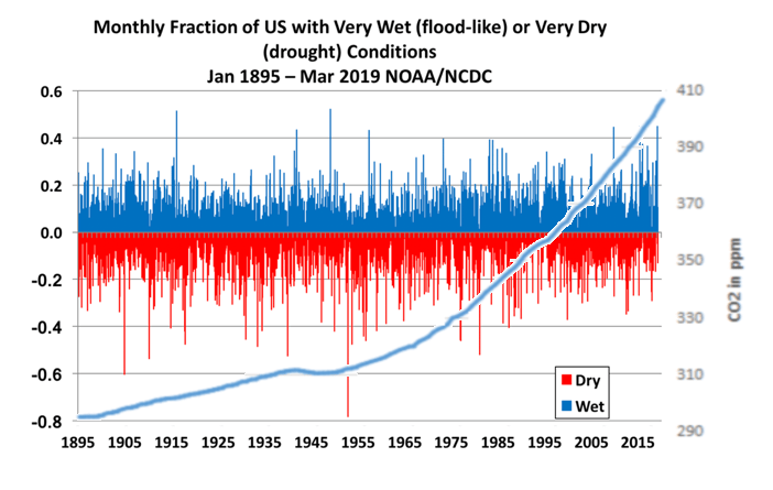
Extreme weather occurrences are likewise used as evidence of an ongoing climate crisis, but again, a study of the available data undercuts that assessment. U.S. tornado activity shows either no increase or a downward trend since 1954. Data on tropical storms, hurricanes, and accumulated cyclone energy (a wind-speed index measuring the overall strength of a given hurricane season) reveal little change since satellite measurements of the phenomena began in the early 1970s. The Palmer Drought Severity Index shows no trend since 1895.

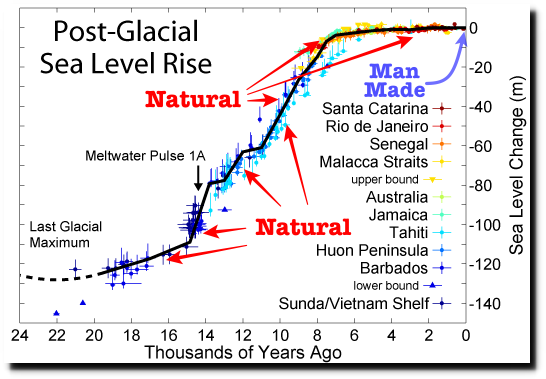
Rising sea levels are another frequently cited example of the impending climate crisis. And yet sea levels have been rising since at least the mid-19th century, a phenomenon unlikely to have been caused only by human activity. The earth has been warming due to both natural and anthropogenic causes, resulting in some melting of sea ice, and a thermal expansion of sea water; the degree to which rising sea level has been caused by man is unknown. And the current rate of sea-level rise as measured by the satellites is 3.3 millimeters per year, or about 13 inches over the course of a century. Will that yield a crisis?

The data reported by the National Oceanic and Atmospheric Administration show that temperatures have risen and fallen since 1850, with an overall upward movement of about 1 degree C for 1850 through 2020. The 1910-1945 warming—which was very roughly the same magnitude as that observed from the mid-1970s through about 2000—is of particular interest in that it cannot be explained by higher greenhouse-gas concentrations, which increased from 300 parts per million to 310 parts per million over that period. This reinforces the commonsense observation that temperatures result from some combination of natural and anthropogenic influences, but alarmist reports seldom if ever suggest that there is any cause of warming other than the latter.
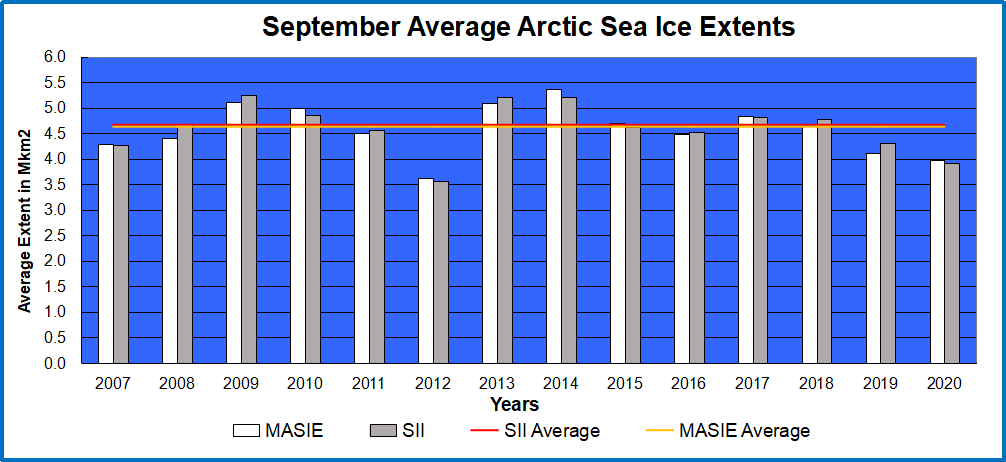
Changes in the extents of Arctic and Antarctic sea ice also raise questions about the importance of moderate warming. Since 1979, Arctic sea ice has declined relative to the 30-year average (again, the degree to which this is the result of anthropogenic factors is not known). Meanwhile, Antarctic sea ice has been growing relative to the 30-year average, and the global sea-ice total has remained roughly constant since 1979.

It is important to recognize that the assumption of many politicians, environmental groups, media sources like the New York Times, and no small number of scientist-activists—that humans are the single most significant cause of climate change—is unsupported by the available science. Such an absence of evidence should produce humility among this group, but it seems to foster more alarmism. At the very least, it should make Americans think twice before embracing radical solutions to a supposed problem that may not be important.

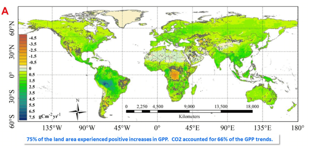
Spatial pattern of trends in Gross Primary Production (1982- 2015). Source: Sun et al. 2018.

Much of the mainstream press has touted, loudly, the alarmist conclusions of the latest IPCC report—amusingly, the IPCC AR6 provides a “Headlines Statements” link to assist alarmist politicians and media—but that reporting has obscured its problems, very real and very large. The report concedes that the mainstream climate models on the whole overstate warming for any given set of parameters and assumptions, but it then relies on those models for predictions about the future.

Figure 8: Warming in the tropical troposphere according to the CMIP6 models. Trends 1979–2014 (except the rightmost model, which is to 2007), for 20°N–20°S, 300–200 hPa. John Christy (2019)

The report concedes as well that the most extreme among its alternative scenarios— “RCP8.5”—has a likelihood that “is considered low,” but then uses RCP8.5 more than any other scenario. The report pretends to measure separately the magnitudes of natural and anthropogenic warming, but in reality does not do so (see Figure SPM.2); instead, it assumes away natural influences, which are asserted to have an average effect of zero. The IPCC models in summary have only two important variables: greenhouse gases, which have a warming effect, and sulfate aerosols, which have a cooling effect. That is why the IPCC models cannot explain the warming observed from 1910-1945. IPCC assumes, but does not attempt to model, a zero effect of sunlight variation, volcanic eruptions, and other such natural phenomena.

The fact is that we don’t understand all the elements in the complex climate system—the effects of clouds alone are understood poorly—and it is beyond irresponsible to adopt policies on the basis of flawed model projections that would slow economic growth in the US and elsewhere. That is a senseless and dangerous policy, which will only hurt people around the world who are striving to create better lives for themselves and their families.


Fear Not Warming from CO2

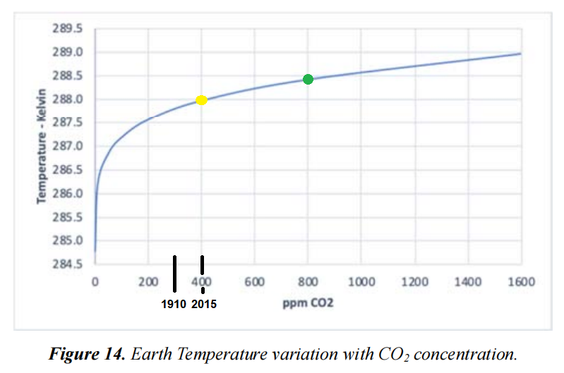
Yellow dot is the present day ppm CO2 and the Green dot is double present ppm CO2. NASA estimates CO2 was 300 ppm in 1910 and 400 ppm in 2015. Exhibit from Coe et al. with added information.

Consensus climate science asserts as given a difference of 33°K between earth surface temperature average 288°K and top of the atmosphere temperature average 255°K. It further claims that IR active gases in the atmosphere (so-called “greenhouse gases”) cause the entire 33°K by their absorption of IR emitted from the earth.  A recent peer-reviewed paper took without challenging that presumption and proceeded to attribute the warming effect to the various GHGs:  H2O, CO2, CH4, and N2O.  The researchers are expert with measures of atmospheric radiation activity and use of the HITRAN database.  The paper is The Impact of CO2, H2O and Other “Greenhouse Gases” on Equilibrium Earth Temperatures by David Coe et al.  Excerpts in italics with my bolds.  H\T Paul Homewood

Abstract

It has long been accepted that the “greenhouse effect”, where the atmosphere readily transmits short wavelength incoming solar radiation but selectively absorbs long wavelength outgoing radiation emitted by the earth, is responsible for warming the earth from the 255K effective earth temperature, without atmospheric warming, to the current average temperature of 288K. It is also widely accepted that the two main atmospheric greenhouse gases are H2O and CO2.

What is surprising is the wide variation in the estimated warming potential of CO2, the gas held responsible for the modern concept of climate change. Estimates published by the IPCC for climate sensitivity to a doubling of CO2 concentration vary from 1.5 to 4.5°C based upon a plethora of scientific papers attempting to analyse the complexities of atmospheric thermodynamics to determine their results.

The aim of this paper is to simplify the method of achieving a figure for climate sensitivity not only for CO2, but also CH4 and N2O, which are also considered to be strong greenhouse gases, by determining just how atmospheric absorption has resulted in the current 33K warming and then extrapolating that result to calculate the expected warming due to future increases of greenhouse gas concentrations.

The HITRAN database of gaseous absorption spectra enables the absorption of earth radiation at its current temperature of 288K to be accurately determined for each individual atmospheric constituent and also for the combined absorption of the atmosphere as a whole. From this data it is concluded that H2O is responsible for 29.4K of the 33K warming, with CO2 contributing 3.3K and CH4 and N2O combined just 0.3K. Climate sensitivity to future increases in CO2 concentration is calculated to be 0.50K, including the positive feedback effects of H2O, while climate sensitivities to CH4 and N2O are almost undetectable at 0.06K and 0.08K respectively. This result strongly suggests that increasing levels of CO2 will not lead to significant changes in earth temperature and that increases in CH4 and N2O will have very little discernable impact.

Discussion

Unlike water vapour, the mean CO2 concentration will remain constant at all atmospheric levels, although its density will reduce as altitude increases and pressure and temperature decrease. CO2 concentration however will vary considerably with location and with seasons, as biospheric photosynthesis removes substantial seasonal amounts of CO2 from the atmosphere. A mean level of 400ppm has been assumed for the following calculations of atmospheric absorptivity. Similarly, CH4 and N2O concentrations will be considered to remain constant at current average levels of 1.8ppm and 0.32ppm respectively.

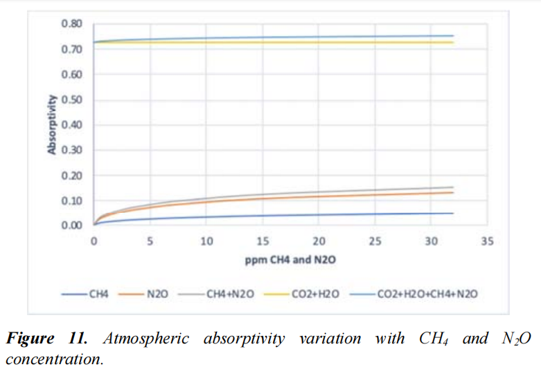
CH4 and N2O are indeed very powerful absorbers of infra-red radiation. Increasing the concentrations of each gas to 30ppm (a 16fold increase in the case of CH4 and an almost
100fold increase in N2O) would result in a combined absorption of 15%, close to the value of 18% for 400ppm of CO2. The combined absorptive impact in the presence of
H2O and CO2 however reduces this absorption to less than 3% as can be seen in Figure 11 due to the overlap of the absorption bands of CO2 and H2O. It would thus take a huge increase in atmospheric concentrations of these gases to have any significant impact on total atmospheric infra-red absorption.

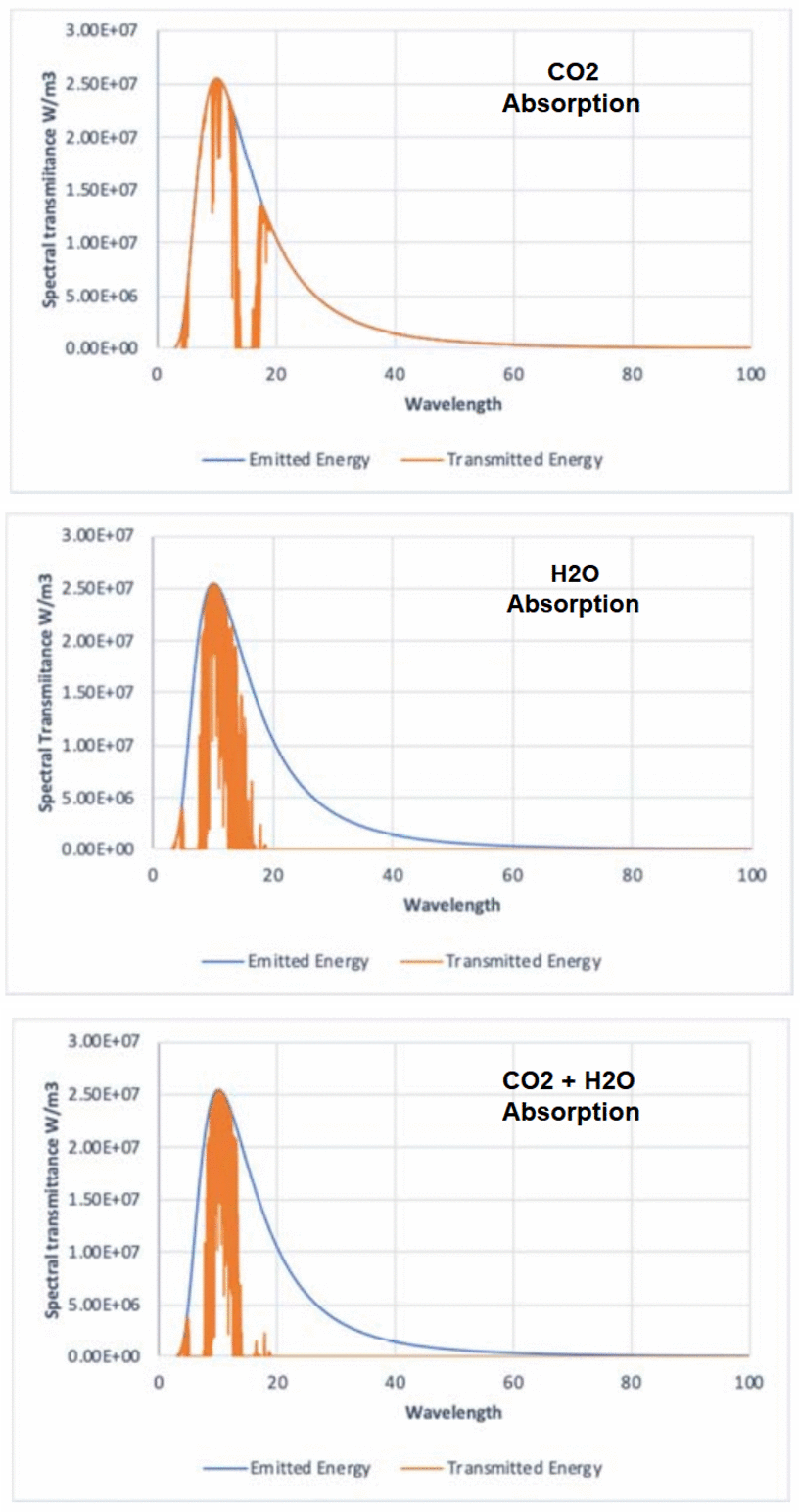
Figures 4, 5 and 6 show the transmission of the spectral radiation Eλ, through current atmospheric concentrations of CO2 and H2O and through the combination of the two gases. Absorptivities of both CO2 and H2O, as well as CH4 and N2O, have been determined over the range 3 to 100µm to a resolution of 0.1cm-1. It is clear that significant amounts of radiated energy are absorbed by both CO2 and H2O. It is also clear that there is considerable overlap of the absorption bands of CO2 and H2O with the H2O absorption being the dominant factor.

Coe et al. Figures 4, 5 and 6.

It is of some interest to calculate the increase in temperature that has occurred due to the increase in atmospheric CO2 levels from the 280ppm prior at the start of the industrial revolution to the current 420ppm registered at the Mona Loa Observatory. (K. W. Thoning et. al. 2019) [17]. The HITRAN calculations show that atmospheric absorptivity has increased from 0.727 to 0.730 due to the increase of 140ppm CO2, resulting in a temperature increase of 0.24Kelvin. This is, therefore, the full extent of anthropogenic global warming to date.

Conclusions

From this it follows that the 33Kelvin warming of the earth from 255Kelvin, widely accepted as the zero-atmosphere earth temperature, to the current average temperature of 288Kelvin, is a 29.4K increase attributed to H2O, 3.3K to CO2 and 0.3K to CH4 and N2O combined. H2O is by far the dominant greenhouse gas, and its atmospheric concentration is determined solely by atmospheric temperature. Furthermore, the strength of the H2O infra-red absorption bands is such that the radiation within those bands is quickly absorbed in the lower atmosphere resulting in further increases in H2O concentrations having little further effect upon atmospheric absorption and hence earth temperatures. An increase in average Relative Humidity of 1% will result in a temperature increase of 0.03Kelvin.

By comparison CO2 is a bit player. It however does possess strong spectral absorption bands which, like H2O, absorb most of the radiated energy, within those bands, in the lower atmosphere. It also suffers the big disadvantage that most of its absorption bands are overlapped by those of H2O thus reducing greatly its effectiveness. In fact, the climate sensitivity to a doubling of CO2 from 400ppm to 800ppm is calculated to be 0.45 Kelvin. This increases to 0.50 Kelvin when feedback effects are taken into account. This figure is significantly lower than the IPCC claims of 1.5 to 4.5 Kelvin.

The contribution of CH4 and N2O is miniscule. Not only have they contributed a mere 0.3Kelvin to current earth temperatures, their climate sensitivities to a doubling of their present atmospheric concentrations are 0.06 and 0.08 Kelvin respectively. As with CO2 their absorption spectra are largely overlapped by the H2O spectra again substantially reducing their impact.

It is often claimed that a major contributor to global warming is the positive feedback effect of H2O. As the atmosphere warms, the atmospheric concentration of H2O also increases, resulting in a further increase in temperature suggesting that a tipping point might eventually be reached where runaway temperatures are experienced. The calculations in this paper show that this is simply not the case. There is indeed a positive feedback effect due to the presence of H2O, but this is limited to a multiplying effect of 1.183 to any temperature increase. For example, it increases the CO2 climate sensitivity from 0.45K to 0.53K.

A further feedback, however, is caused by a reduction in atmospheric absorptivity as the spectral radiance of the earth’s emitted energy increases with temperature, with peak emissions moving slightly towards lower radiation wavelengths. This causes a negative feedback with a temperature multiplier of 0.9894. This results in a total feedback multiplier of 1.124, reducing the effective CO2 climate sensitivity from 0.53 to 0.50 Kelvin.

Feedback effects play a minor role in the warming of the earth. There is, and never can be, a tipping point. As the concentrations of greenhouse gases increase, the temperature sensitivity to those increases becomes smaller and smaller. The earth’s atmosphere is a near perfect example of a stable system. It is also possible to attribute the impact of the increase in CO2 concentrations from the pre-industrial levels of 280ppm to the current 420ppm to an increase in earth mean temperature of just 0.24Kelvin, a figure entirely consistent with the calculated climate sensitivity of 0.50 Kelvin.

The atmosphere, mainly due to the beneficial characteristics and impact of H2O absorption spectra, proves to be a highly stable moderator of global temperatures. There is no impending climate emergency and CO2 is not the control parameter of global temperatures, that accolade falls to H2O. CO2 is simply the supporter of life on this planet as a result of the miracle of photosynthesis.

Footnote:

Coe et al. confirm what Ångström showed experimentally a century ago. He stated in 1900:
“Under no circumstances should carbon dioxide absorb more than 16 percent of terrestrial radiation, and the size of this absorption varies quantitatively very little, as long as there is not less than 20 percent of the existing value.”  See Pick Your A-Team: Arrhenius or Ångström

Independently, W. A. van Wijngaarden, W. Happer published findings this year similar to Coe et al. in their study Relative Potency of Greenhouse Molecules

World of Climate Change Infographics

Raymond of RiC-Communications studio created infographics on CO2 for improving public awareness.  He produced 13 interesting slides which are presented in the post World of CO2 Infographics  A second project was created on a related theme The World of Climate Change comprising six charts, including one regarding Alpine glacier studies by two prominent geologists.  In addition, Raymond was able to consult the work of  these two experts in their native German language.

This project is The World of Climate Change

Infographics can be helpful, in making things simple to understand. Climate change is a complex topic with a lot of information and statistics. These simple step by step charts are to better understand what is occurring naturally and what could be caused by humans. What is cause for alarm and what isn’t cause for alarmism if at all. Only through learning is it possible to get the big picture so as to make the right decisions for the future.

Images are available at these links:

The+World+of+CO2 CO2 charts

The+World+of+Climate+Change Charts

World+of+Ice+Ages Charts

The+World+of+Energy Charts

– N° 1 600 million years of global temperature change
– N° 2 Earth‘s temperature record for the last 400,000 years
– N° 3 Holocene period and average northern hemispheric temperatures
– N° 4 140 years of global mean temperature
– N° 5 120 m of sea level rise over the past 20‘000 years
– N° 6 Eastern European alpine glacier history during the Holocene period.


03_infographic_wocc-1

04_infographic_wocc

Summer Temperatures (May – September) A rise in temperature during a warming period will result in a glacier losing more surface area or completely vanishing. This can happen very rapidly in only a few years or over a longer period of time. If temperatures drop during a cooling period and summer temperatures are too low, glaciers will begin to grow and advance with each season. This can happen very rapidly or over a longer period in time. Special thanks to Prof. em. Christian Schlüchter / (Quartärgeologie, Umweltgeologie) Universität Bern Institut für Geologie His work is on the Western Alps and was so kind to help Raymond make this graphic as correct as possible.

Comment:

This project explored information concerning how aspects of the world climate system have changed in the past up to the present time.  Understanding the range of historical variation and the factors involved is essential for anticipating how future climate parameters might fluctuate.

For example:

The Climate Story (Illustrated) looks at the temperature record.

H20 the Gorilla Climate Molecule looks at precipitation patterns.

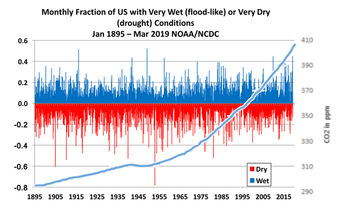
Data vs. Models #2: Droughts and Floods looks at precipitation extremes.

Data vs. Models #3: Disasters looks at extreme weather events.

Data vs. Models #4: Climates Changing looks at boundaries of defined climate zones.

And in addition, since Chart #5 features the Statue of Liberty, here are the tidal gauge observations there compared to climate model projections:

NYC past & projected 2020

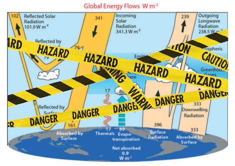
Beware Energy Balance Cartoons

Figure 1. The global annual mean energy budget of Earth’s climate system (Trenberth and Fasullo, 2012.)

Recently in a discussion thread a warming proponent suggested we read this paper for conclusive evidence. The greenhouse effect and carbon dioxide by Wenyi Zhong and Joanna D. Haigh (2013) Imperial College, London. Indeed as advertised the paper staunchly presents IPCC climate science. Excerpts in italics with my bolds.

IPCC Conception: Earth’s radiation budget and the Greenhouse Effect

The Earth is bathed in radiation from the Sun, which warms the planet and provides all the energy driving the climate system. Some of the solar (shortwave) radiation is reflected back to space by clouds and bright surfaces but much reaches the ground, which warms and emits heat radiation. This infrared (longwave) radiation, however, does not directly escape to space but is largely absorbed by gases and clouds in the atmosphere, which itself warms and emits heat radiation, both out to space and back to the surface. This enhances the solar warming of the Earth producing what has become known as the ‘greenhouse effect’. Global radiative equilibrium is established by the adjustment of atmospheric temperatures such that the flux of heat radiation leaving the planet equals the absorbed solar flux.

The schematic in Figure 1, which is based on available observational data, illustrates the magnitude of these radiation streams. At the Earth’s distance from the Sun the flux of radiant energy is about 1365Wm−2 which, averaged over the globe, amounts to 1365/4 = 341W for each square metre. Of this about 30% is reflected back to space (by bright surfaces such as ice, desert and cloud) leaving 0.7 × 341 = 239Wm−2 available to the climate system. The atmosphere is fairly transparent to short wavelength solar radiation and only 78Wm−2 is absorbed by it, leaving about 161Wm−2 being transmitted to, and absorbed by, the surface. Because of the greenhouse gases and clouds the surface is also warmed by 333Wm−2 of back radiation from the atmosphere. Thus the heat radiation emitted by the surface, about 396Wm−2, is 157Wm−2 greater than the 239Wm−2 leaving the top of the atmosphere (equal to the solar radiation absorbed) – this is a measure of ‘greenhouse trapping’.

Why This Line of Thinking is Wrong and Misleading
Principally, the Earth is not a disk illuminated 24/7 by 1/4 of solar radiant energy. 

That disk in the cartoon denies the physical reality of a rotating sphere, and completely distorts the energy dynamics.  Christos Vournas addresses this issue directly in deriving his planetary temperature equation that corresponds to NASA satellite measurements of planets and moons in our solar system.  Previous posts provide background for this one focusing on the radiant heating of the rotating water planet we call Earth (though Ocean would be more accurate).  See How to Calculate Planetary Temperatures and Earthshine and Moonshine: Big Difference.  

i285978589391372458._szw1280h1280_-1

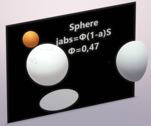
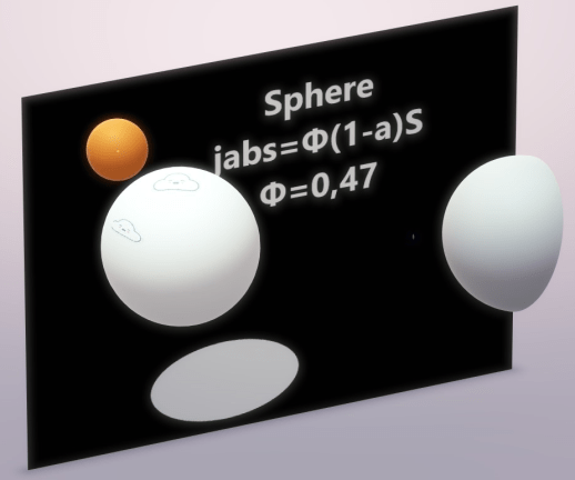
Φ – is the dimensionless Solar Irradiation accepting factor. It recognizes that a sphere’s surface absorbs the incident solar irradiation not as a disk of the same diameter, but accordingly to its spherical shape. For a smooth spherical surface Φ = 0,47

The classical blackbody surface properties

A blackbody planet surface is meant as a classical blackbody surface approaching.  Here are the blackbody’s properties:

1. Blackbody does not reflect the incident on its surface radiation. Blackbody absorbs the entire radiation incident on its surface.

2. Stefan-Boltzmann blackbody emission law is:   Je = σ*Τe⁴

Notice:

Te is the blackbody’s temperature (surface) at every given moment. When the blackbody is not irradiated, the classical blackbody gradually cools down, gradually emitting away its accumulated energy.  The classical blackbody concept assumes blackbody’s surface being warmed by some other incoming irradiation source of energy – see the Sun’s paradigm.  Sun emits like a blackbody, but it emits its own inner energy source’s energy. Sun is not considered as an irradiation receiver. And sun has a continuous stable temperature.

Therefore we have here two different blackbody theory concepts.

a. The blackbody with the stable surface temperature due to its infinitive inner source (sun, stars).
b. The blackbody with no inner energy source.

This blackbody’s emission temperature relies on the incoming outer irradiation only.

Also in the classical blackbody definition it is said that the irradiation incident on the blackbody is totally absorbed, warms the blackbody and achieves an equilibrium emission temperature Te.  It is an assumption.

This assumption, therefore, led to the next assumption: the planet like a blackbody emitting behavior.  And, consequently, it resulted to the planet’s Te equation, in which it is assumed that planet’s surface is interacting with the incoming irradiation as being in a uniform equilibrium temperature.

Consequently it was assumed that planet’s surface had a constant equilibrium temperature (which was only the incident solar irradiation dependent value) and the only thing the planet’s surface did was to emit in infrared spectrum out to space the entire absorbed solar energy.

3. When irradiated, the blackbody’s surface has emission temperature according to the Stefan-Boltzmann Law:

Te = (Total incident W /Total area m² *σ)¹∕ ⁴ K

σ = 5,67*10⁻⁸ W/m²K⁴, the Stefan-Boltzmann constant.

Notice: This emission temperature is only the incoming irradiation energy depended value. Consequently when the incoming irradiation on the blackbody’s surface stops, at that very moment the blackbody’s emission temperature disappears.  It happens because no blackbody’s surface accumulates energy.

4. Blackbody interacts with the entire incident on the blackbody’s surface radiation.

5. Blackbody’s emission temperature depends only on the quantity of the incident radiative energy per unit area.

6. Blackbody is considered only as blackbody’s surface physical properties. Blackbody is only a surface without “body”.

7. Blackbody does not consist from any kind of a matter. Blackbody has not a mass. Thus blackbody has not a specific heat capacity.  Blackbody’s cp = 0.

8. Blackbody has surface dimensions. So blackbody has the radiated area and blackbody has the emitting area.

9. The entire blackbody’s surface area is the blackbody’s emitting area.

10. The blackbody’s surface has an infinitive conductivity.

11. All the incident on the blackbody’s surface radiative energy is instantly and evenly distributed upon the entire blackbody’s surface.

12. The radiative energy incident on the blackbody’s surface the same very instant the blackbody’s surface emits this energy away.

A Real Planet is Not a Blackbody

But what happens there on the rotating real planet’s surface?

The rotating real planet’s surface, when it turns to the sunlit side, is an already warm at some temperature, from the previous day, planet’s surface.

Thus, when assuming the planet’s surface behaving as a blackbody, we face the combination of two different initial blackbody surfaces.

a. The one with an inner energy source.

And

b. The one warmed by an outer irradiation.

The Real Planet’s Surface Properties:

1. The planet’s surface has not an infinitive conductivity. Actually the opposite takes place. The planet’s surface conductivity is very small, when compared with the solar irradiation intensity and the planet’s surface infrared emissivity intensity.

2. The planet’s surface has thermal behavior properties. The planet’s surface has a specific heat capacity, cp.

3. The incident on the planet solar irradiation is not being distributed instantly and evenly on the entire planet’s surface area.

4. Planet does not accept the entire solar irradiation incident in planet’s direction. Planet accepts only a small fraction of the incoming solar irradiation. This happens because of the planet’s albedo, and because of the planet’s smooth and spherical surface reflecting qualities, which we refer to as “the planet’s solar irradiation accepting factor Φ”.

Planet reflects the (1-Φ + Φ*a) portion of the incident on the planet’s surface solar irradiation.  And  Planet absorbs only the Φ(1 – a) portion of the incident on the planet’s surface solar irradiation.

Here “a” is the planet’s average albedo and “Φ” is the planet’s solar irradiation accepting factor.

For smooth planet without thick atmosphere, Earth included, Φ=0,47

5. Planet’s surface has not a constant intensity solar irradiation effect. Planet’s surface rotates under the solar flux. This phenomenon is decisive for the planet’s surface infrared emittance distribution.

The real planet’s surface infrared radiation emittance distribution intensity is a planet’s rotational speed dependent physical phenomenon.

Vournas fig1

Φ factor explanation

The Φ – solar irradiation accepting factor – how it “works”. It is not a planet specular reflection coefficient itself.

There is a need to focus on the Φ factor explanation. Φ factor emerges from the realization that a sphere reflects differently than a flat surface perpendicular to the Solar rays.

It is very important to understand what is really going on with planets’ solar irradiation reflection.

There is the specular reflection and there is the diffuse reflection.

The planet’s surface Albedo “a” accounts for the planet’s surface diffuse reflection. Albedo is defined as the ratio of the scattered SW to the incident SW radiation, and it is very much precisely measured (the planet Bond Albedo).

So till now we didn’t take in account the planet’s surface specular reflection. A smooth sphere, as some planets are, are invisible in space and have so far not been detected and the specular reflection not measured . The sphere’s specular reflection cannot be seen from the distance, but it can be seen by an observer situated on the sphere’s surface.

i285978589389395456._szw1280h1280_

Thus, when we admire the late afternoon sunsets on the sea we are blinded from the brightness of the sea surface glare. It is the surface specular reflection that we see then.

Jsw.absorbed = Φ*(1-a) *Jsw.incoming

For a planet with albedo a = 0 (completely black surface planet) we would have

Jsw.reflected = [1 – Φ*(1-a)]*S *π r² =

Jsw.reflected = (1 – Φ) *S *π r²

For a planet which captures the entire incident solar flux (a planet without any outgoing specular reflection) we would have Φ = 1

Jsw.absorbed = Φ*(1-a) *Jsw.incoming

Jsw.reflected = a *Jsw.incoming

And

For a planet with Albedo a = 1 , a perfectly reflecting planet

Jsw.absorbed = 0 (no matter what is the value of Φ)

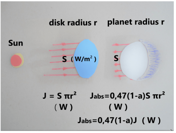
In general:  The fraction left for hemisphere to absorb is  Jabs = Φ (1 – a ) S π r²

We have Φ for different planets’ surfaces varying  0,47 ≤ Φ ≤ 1

And we have surface average Albedo “a” for different planets’ varying  0 ≤ a ≤ 1

Notice:

Φ is never less than 0,47 for planets (spherical shape).

Also, the coefficient Φ is “bounded” in a product with (1 – a) term, forming the Φ(1 – a) product cooperating term. Thus Φ and Albedo are always bounded together.

The Φ(1 – a) term is a coupled physical term.

The Φ(1 – a) term “translates” the absorption of a disk into the absorption of a smooth hemisphere with the same radius.

When covering a disk with a hemisphere of the same radius the hemisphere’s surface area is 2π r². The incident Solar energy on the hemisphere’s area is the same as on the disk:  Jdirect = π r² S

But the absorbed Solar energy by the hemisphere’s area of 2π r² is:  Jabs = Φ*( 1 – a) π r² S

It happens because a smooth hemisphere of the same radius “r” absorbs only the Φ*(1 – a)S portion of the directly incident on the disk of the same radius Solar irradiation.

In spite of hemisphere having twice the area of the disk, it absorbs only the Φ*(1 – a)S portion of the directly incident on the disk Solar irradiation.

Gaseous Planets

Φ = 1 for gaseous planets, as Jupiter, Saturn, Neptune, Uranus, Venus, Titan.

Gaseous planets do not have a surface to reflect radiation. The solar irradiation is captured in the thousands of kilometers gaseous abyss. The gaseous planets have only the albedo “a”.

Heavy Cratered Planets

Φ = 1 for heavy cratered planets, as Calisto and Rhea ( not smooth surface planets, without atmosphere ).

The heavy cratered planets have the ability to capture the incoming light in their multiple craters and canyons. The heavy cratered planets have only the albedo “a”.

That is why the albedo “a” and the factor “Φ” we consider as different values. Both of them, the albedo “a” and the factor “Φ” cooperate in the

Energy in = Φ(1 – a) left side of the Planet Radiative Energy Budget.

Conclusively, the Φ -Factor is not the planet specular reflection portion itself.

The Φ -Factor is the Solar Irradiation Accepting Factor (in other words, Φ is the planet surface shape and roughness coefficient).

Bottom Line

What is going on here is that instead of Jabs.earth = 0,694* 1.361 π r² ( W ) we should consider Jabs.earth = 0,326* 1.361 π r² ( W ).

Averaged on the entire Earth’s surface we obtain:

Jsw.absorbed.average = [ 0,47*(1-a)*1.361 W/m² ] /4 =

= [ 0,47*0,694*1.361W/m² ] /4 = 444,26 W/m2 /4 = 111,07 W/m²

Jsw.absorbed.average = 111,07 W/m² or 111 W/m²

Example:  Comparing Earth and Europa

Earth / Europa satellite measured mean temperatures 288 K and 102 K comparison
All the data below are satellites measurements. All the data below are observations.

Planet Earth Europa
Tsatmean  288 K 102 K
R 1 AU 5.2044 AU
1/R² 1 0,0369
N 1 1/3.5512 rot/day
a 0.3 0.63
(1-a) 0.7 0.37
coeff 0.91469 0.3158

We could successfully compare Earth /Europa ( 288 K /102 K ) satellite measured mean temperatures because both Earth and Europa (moon of Jupiter) have two identical major features.

Φearth = 0,47 because Earth has a smooth surface and Φeuropa = 0,47 because Europa also has a smooth surface.

cp.earth = 1 cal/gr*°C, it is because Earth has a vast ocean. Generally speaking almost the whole Earth’s surface is wet. We can call Earth a Planet Ocean.  Europa is an ice-crust planet without atmosphere, Europa’s surface consists of water ice crust, cp.europa = 1cal/gr*°C.

The table below shows how well the universal equation estimates temperatures of planets and moons measured by NASA.

Planet Φ Te.correct  [(β*N*cp)¹∕ ⁴]¹∕ ⁴ Tmean  Tsat
Mercury  0.47 364 0.8953 325.83 340
Earth  0.47 211 1.3680 287.74 288
Moon  0.47 224 0.9978 223.35 220
Mars  0.47 174 1.2270 213.11 210
Io  1 95.16 1.1690 111.55 110
Europa  0.47 78.83 1.2636 99.56 102
Ganymede 0.47 88.59 1.2090 107.14 110
Calisto  1 114.66 1.1471 131.52 134 ±11
Enceladus  1 55.97 1.3411 75.06 75
Tethys  1 66.55 1.3145 87.48 86 ± 1
Titan  1 84.52 1.1015 96.03 93.7
Pluto  1 37 1.1164 41.60 44
Charon  1 41.9 1.2181 51.04 53
My Comment:

This post explains why it is an error to treat Earth (or any planetary body) as a classic blackbody in either the absorption of incident energy or in the emission of radiation.  Thus the typical energy balance cartoons are not funny, they are false and misleading.  A further error arises in claiming that greenhouse gases like CO2 in the atmosphere cause surface warming by trapping Earth radiation and slowing the natural cooling.  This fallacy is addressed directly in a previous post Why CO2 Can’t Warm the Planet.

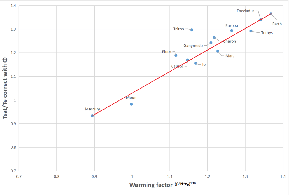
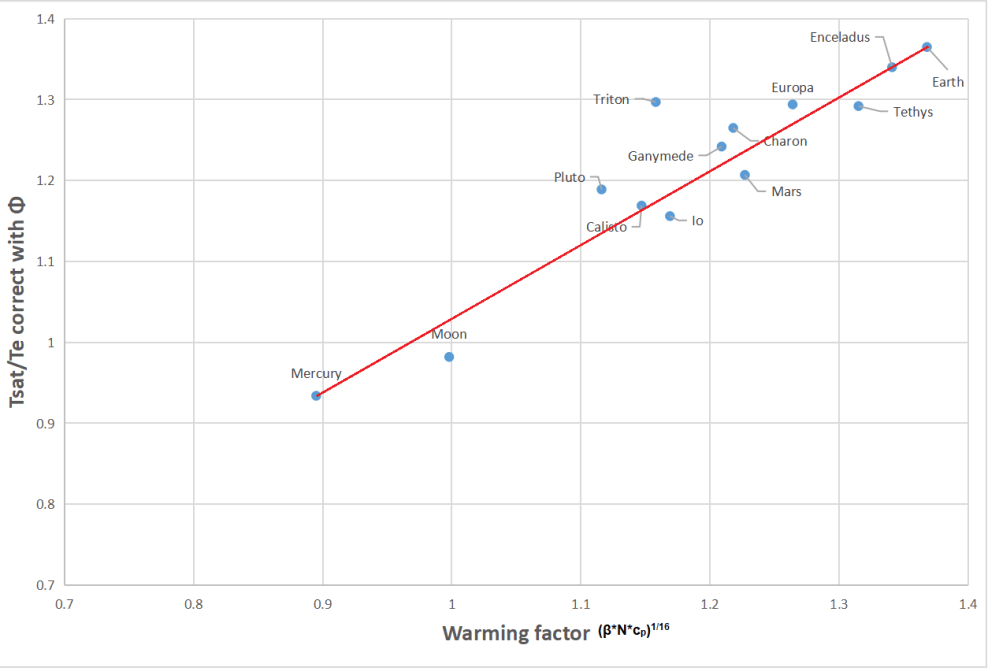
The table above and graph below show that Earth’s warming factor is correctly calculated despite ignoring any effect from its thin atmosphere.

i285978589399740131._szw1280h1280_-1

Earthshine and Moonshine: Big Difference

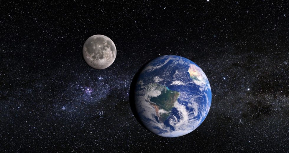
earth moon highres

A previous post elaborated a rigorous equation from Christos Vournas for calculating surface temperatures of planets or moons, for comparison with NASA satellite measurements of such bodies in our solar system.  That post is How to Calculate Planetary Temperatures.

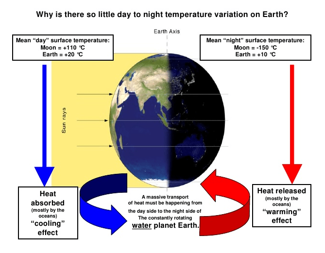
The image above presents the huge disparity in day and night temperatures between Earth and its Moon, and notes the role of ocean heat transport.  But as I have learned from Christos, there is much more to the story, and this post discusses these deeper implications.  He adds the rotational factor and its impact upon the radiation emitted by both bodies, ie. Earthshine and Moonshine (though obviously it is not simply visible light).  Excerpts from Vournas are in italics with my bolds.

moon-earth-980x520-1

Moon and Earth – so close to each other – and so much different…

Moon is in our immediate neighborhood

Moon rotates around its axis at a slow rate of 29.5 days.  The day on the Moon is 14.75 earth days long, and the night on the Moon is also 14.75 Earth days long. 

Moon is in our immediate neighborhood. So Moon is at the same distance from the sun, as Earth, R=1 AU (astronomical unit).  The year average solar irradiation intensity on the top of atmosphere for Moon and Earth is the same

So = 1361 W/m².

We say “on the top of the atmosphere”, it means the solar intensity which reaches a celestial body and then falls on it. For certain then, during these 14.75 earth days long lunar day the Moon’s surface gets warmed at much higher temperatures than the Earth.

There is the Planet Surface Rotational Warming Phenomenon

I’ll try here in few simple sentences explain the very essence of how the planet rotational warming Phenomenon occurs.

Lets consider two identical planets F and S at the same distance from the sun.  Let’s assume the planet F spins on its axis Faster, and the planet S spins on its axis Slower.  Both planets F and S get the same intensity solar flux on their sunlit hemispheres. Consequently both planets receive the same exact amount of solar radiative energy.

The slower rotating planet’s S sunlit hemisphere surface gets warmed at higher temperatures than the faster rotating planet’s F sunlit hemisphere. The surfaces emit at σT⁴ intensity – it is the Stefan-Boltzmann emission law.

Thus the planet S emits more intensively from the sunlit side than the planet F.  There is more energy left for the planet F to accumulate then.  That is what makes the faster rotating planet F on the average a warmer planet.

That is how the Planet Surface Rotational Warming Phenomenon occurs.

And it becomes very cold on the Moon at night

Moon gets baked hard during its 14,75 earth days long lunar day.  And Moon also emits hard from its very hot daytime surface.  What else can the very hot surface do but to emit hard, according to the Stefan-Boltzmann emission Law.  The very hot surface emits in fourth power of its very high absolute temperature.

Jemit ~ T⁴

A warm object in space loses heat via emission. The hotter is the object, the faster it loses heat.  So there is not much energy left to emit during the 14.75 earth days long lunar night.

The Table below shows the implications:

Planet Tsat mean Rotations Tmin Tmax
Mercury 340 K 1/176 100K 700K
Earth 288 K 1
Moon 220 Κ 1/29.5 100K 390K
Mars 210 K 0.9747 130K 308K
Comparing Mars and Mercury

The closest to the sun planet Mercury receives 15.47 times stronger solar irradiation intensity than the planet Mars does.  However on the Mercury’s dark side Tmin.mercury = 100 K, when on the Mars’ dark side Tmin.mars = 130 K.

These are observations, these are from satellites the planets’ temperatures measurements.  And they cannot be explained otherwise but by the planet Mars’ 171.5 times faster rotation than planet Mercury’s spin.

Earth-Moon temperatures comparison -why the differences

The faster (than Moon) Earth’s rotation smooths the average heat. The higher (than Moon) Earth’s surface specific heat capacity(oceanic waters vs dry regolith), also smooths the average heat. Consequently the daytime Earth’s surface temperature (compared to Moon) lessens, and the nighttime Earth’s surface temperature (compared to Moon) rises. Earth receives the same amount of solar heat (per unit area) from sun as Moon – for the same albedo. And Earth emits the same amount of solar heat, as the Moon does.

But something else very interesting happens.

It is the difference between Earth’s and Moon’s emitting temperatures. At the daytime Earth’s surface is warmed at a much lower temperatures and therefore at the daytime Earth’s surface emits IR radiation at a much lower intensities. So the intensity of Earth’s daytime IR radiation is much lower (than Moon’s).

As a result, there is a great amount of energy – compared to Moon – “saved” on Earth during the daytime emission..  This “saved” energy should be emitted by Earth’s surface during the nighttime then. At the night-time Earth’s surface is warmer than Moon’s and therefore Earth’s surface at night-time is at a higher temperatures.  So the intensity of Earth’s night-time IR radiation is higher.

There is always a balance.  The energy in = the energy out

But again something else very interesting happens.

In order to achieve that balance Earth’s night-time IR emitting intensity should be much higher than the night-time IR emitting intensity of the Moon.  Now we should take notice of the nonlinearity of the Stefan-Boltzmann emission law. Consequently the night-time temperatures on Earth rise higher (compared to Moon) than the daytime temperatures on Earth lessens.

So the average Earth’s surface temperature is warmer (compared to the Moon). Thus Earth’s Tmean.earth = 288 K and Moon’s Tmean.moon = 220 K

The faster rotation and the higher specific heat capacity does not make sun to put more energy in the Earth’s surface. What the faster rotation and the higher specific heat capacity do is to modify the way Earth’s surface emits, the same amount as Moon, of energy (per unit area).

Earth emits IR radiation at lower temperatures during the daytime and at higher temperatures at night-time. Because of the nonlinearity of this process according to the Stefan-Boltzmann emission law, Earth ends up to have on average warmer surface than Moon.

The night-time temperatures on Earth rise higher (compared to Moon) than the day-time temperatures on Earth lessens. Earth receives (for the same albedo and per unit area) the same amount of solar energy as the Moon . This energy is “welcomed” on each planet and processed in a unique way for each planet.

To illustrate the above conclusions I’ll try to demonstrate on the Earth-Moon temperatures comparison rough example:

Surface temperatures

.min……mean……max

Tmin↑↑→T↑mean ←T↓max

Moon…100 K…220 K …390 K

Δ………..+84 K +68 K….- 60 Κ

Earth…184K↑↑.288 K↑.330 K↓

So we shall have for the faster rotating Earth, compared to the Moon:

Tmin↑↑→ T↑mean ← T↓max

+84↑↑→ +68↑mean ← -60↓

The faster a planet rotates (n2>n1) the higher is the planet’s average (mean) temperature T↑mean.

Note:  To emphasize we should mention that Moon’s max and min temperatures are measured on Moon’s equator, and Earth’s max and min temperatures are not.  Earth’s max and min temperatures are measured on continents, and not on oceanic waters. Otherwise the Δmin would have been even bigger and the Δmax would have been much smaller.

This rough example nevertheless illustrates that for the faster rotating and covered with water (higher cp) Earth compared with Moon the average temperature should be higher.

The planet’s faster rotation and the planet’s higher specific heat capacity “cp” not only smooths, but also processes ( Δmin > Δmax ), the same incoming solar heat, but in a different emission pattern.

Earth is warmer because Earth rotates faster and because Earth’s surface is covered with water

We had to answer these two questions:

1. Why Earth’s atmosphere doesn’t affect the Global Warming?

It is proven now by the Planet’s Mean Surface Temperature Equation calculations. There aren’t any atmospheric factors in the Equation. Nevertheless the Equation produces very reasonable results:

Tmean.earth = 287,74 K,  calculated by the Equation, which is the same as the Tsat.mean.earth = 288 K, measured by satellites.

Tmean.moon = 223,35 K, calculated by the Equation, which is almost identical with the Tsat.mean.moon = 220 K, measured by satellites.

2. What causes the Global Warming then?

The Global Warming is happening due to the orbital forcing.

And… what keeps Earth warm at Tmean.earth = 288 K, when Moon is at Tmean.moon = 220 K? Why Moon is on average 68 oC colder? It is very cold at night there and it is very hot during the day…

Earth is warmer because Earth rotates faster and because Earth’s surface is covered with water.
Does the Earth’s atmosphere act as a blanket that warms Earth’s surface?

No, it does not.

.

How to Calculate Planetary Temperatures

i285978589399740131._szw1280h1280_

In the second graph we have the Ratio of Planet Measured Temperature to the Corrected Blackbody Temperature (Tsat /Te.correct). Link [30] In this graph we use in (Tsat /Te.correct) the planet corrected blackbody temperatures – which are the planet effective temperatures Te.correct corrected by the use of the Φ -factor. The Φ = 0,47 for smooth surface planets and moons, and the Φ = 1 for the rough surface planets and moons. As we can see, in the second graph, the red dot planets and the green dot planets have stretched in a linear functional relation according to their Warming Factor = (β*N*cp)^1/16 values. The bigger is the planet’s or moon’s Warming Factor, the higher is the (Tsat /Te.correct) ratio. It is obviously a linearly related function.

On a recent comment thread at Climate Etc. Christos Vournas provided a link to his blog. After spending time reading his articles I made this post to introduce aspects of his studies and thinking that I find persuasive. His home page sets the theme The Planet Surface Rotational Warming Phenomenon. Below are just a few excerpts from Vournas’ blog in italics with my bolds.

[Note:  I have added two additional posts on Vournas findings Earthshine and Moonshine: Big Difference  and Beware Energy Balance Cartoons]

Introduction

My name is Christos J. Vournas, M.Sc. mechanical engineer, living in Athens Greece. I launched this site to have an opportunity to publish my scientific discoveries on the Climate Change.  I have been studying the Planet Earth’s Climate Change since November 2015;

First I discovered the Reversed Milankovitch Cycle.

Then I found the faster a planet rotates (n2>n1) the higher is the planet’s average (mean) temperature T↑mean.

Φ – the next discovery – is the dimensionless Solar Irradiation accepting factor – very important

The further studies led me to discover the Rotating Planet Spherical Surface Solar Irradiation Absorbing-Emitting Universal Law and the Planet’s Without-Atmosphere Mean Surface Temperature Equation.

The Planet Surface Rotational Warming Phenomenon

It is well known that when a planet rotates faster its daytime maximum temperature lessens and the night time minimum temperature rises.

But there is something else very interesting happens. When a planet rotates faster it is a warmer planet. (It happens because Tmin↑↑ grows higher than T↓max goes down)

The faster a planet rotates (n2>n1) the higher is the planet’s average (mean) temperature T↑mean:

Tmin↑↑→ T↑mean ← T↓max

The understanding of this phenomenon comes from a deeper knowledge of the Stefan-Boltzmann Law. It happens so because when rotating faster a planet’s surface has a new radiative equilibrium temperatures to achieve.

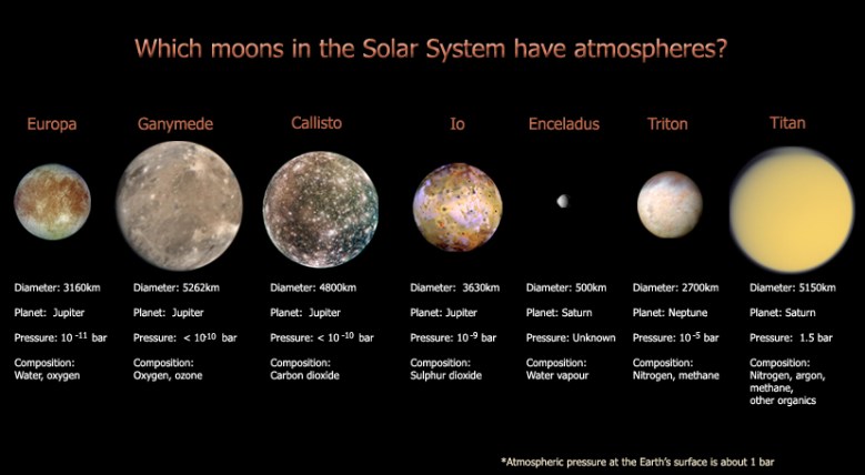
which20moons20have20atmospheres

A Planet Without-Atmosphere Mean Surface Temperature Equation

A Planet Without-Atmosphere Mean Surface Temperature Equation derives from the incomplete Te equation which is based on the radiative equilibrium and on the Stefan-Boltzmann Law.

Using the new equation, the new estimate Tmean closely matches the estimate surface temperatures from satellite observations:

Planet Te.incomp Tmean Tsat.mean
Mercury 437,30K 323,11K 340K
Earth 255K 287,74K 288K
Moon 271K 221,74K 220K
Mars 209,91K 213,59K 210K

We have moved further from the incomplete effective temperature equation

Te = [ (1-a) S / 4 σ ]¹∕ ⁴

(which is in common use right now, but actually it is an incomplete planet Te equation and that is why it gives us very confusing results)

a – is the planet’s surface average albedo

S – is the solar flux, W/m²

σ = 5,67*10⁻⁸ W/m²K⁴, the Stefan-Boltzmann constant

We have discovered the Planet Without-Atmosphere Mean Surface Temperature Equation

Tmean = [ Φ (1-a) S (β*N*cp)¹∕ ⁴ /4σ ]¹∕ ⁴ (1)

The Planet Without-Atmosphere Mean Surface Temperature Equation is also based on the radiative equilibrium and on the Stefan-Boltzmann Law.

The Equation is being completed by adding to the incomplete Te equation the new parameters Φ, N, cp and the constant β.

Φ – is the dimensionless Solar Irradiation accepting factor

Φ – is the dimensionless Solar Irradiation accepting factor.  It is a realizing that a sphere’s surface absorbs the incident solar irradiation not as a disk of the same diameter, but accordingly to its spherical shape.  For a smooth spherical surface Φ = 0,47

i285978589391372458._szw1280h1280_

N – rotations /day, is the planet’s axial spin

cp – cal /gr*oC, is the planet’s surface specific heat capacity

β = 150 days*gr*oC/rotation*cal – is the Rotating Planet Surface Solar Irradiation Absorbing-Emitting Universal Law constant.

The Planet Without-Atmosphere Mean Surface Temperature Equation is also based on the radiative equilibrium and on the Stefan-Boltzmann Law.

But the New Equation doesn’t consider planet behaving as a blackbody, and the New Equation doesn’t state planet having a uniform surface temperature.

Interesting, very interesting what we see here:

Planet Tsat mean Rotations Tmin Tmax
Mercury 340 K 1/176 100K 700K
Earth 288 K 1
Moon 220 Κ 1/29,5 100K 390K
Mars 210 K 0,9747 130K 308K

Earth and Moon are at the same distance from the Sun R = 1 AU.

Earth and Mars have almost the same axial spin N = 1rotation /day.

Moon and Mars have almost the same satellite measured average temperatures 220 K and 210 K.

Mercury and Moon have the same minimum temperature 100 K.

Mars’ minimum temperature is 130 K, which is much higher than for the closer to the Sun Mercury’s and Moon’s minimum temperature 100 K.

The planet’s effective temperature old Te = [ (1-a) S /4σ ]¹∕ ⁴ incomplete equation gives very confusing results.

And the faster rotating Earth and Mars appear to be relatively warmer planets.

We ended up to the following remarkable results

To be honest with you, at the beginning, I was surprised myself with these results.

You see, I was searching for a mathematical approach…

We use more major parameters for the planet’s surface temperature equation.

Planet is a celestial body with more major features when calculating planet effective temperature to consider. The planet without-atmosphere effective temperature calculating formula has to include all the planet’s basic properties and all the characteristic parameters.

3. The planet’s axial spin N rotations/day.

4. The thermal property of the surface (the specific heat capacity cp).

5. The planet’s surface solar irradiation accepting factor Φ ( the spherical surface’s primer solar irradiation absorbing property ).

Altogether these parameters are combined in the Planet’s Without-Atmosphere Surface Mean Temperature Equation:

Tmean.planet = [ Φ (1-a) So (1/R²) (β*N*cp)¹∕ ⁴ /4σ ]¹∕ ⁴ (1)

Earth’s Without-Atmosphere Mean Surface Temperature Equation
Tmean.earth

So = 1.361 W/m² (So is the Solar constant)

Earth’s albedo: aearth = 0,306

Earth is a rocky planet, Earth’s surface solar irradiation accepting factor Φearth = 0,47 (Accepted by a Smooth Hemisphere with radius r sunlight is S*Φ*π*r²(1-a), where Φ = 0,47)

β = 150 days*gr*oC/rotation*cal – is a Rotating Planet Surface Solar Irradiation Absorbing-Emitting Universal Law constant

N = 1 rotation /per day, is Earth’s sidereal rotation spin

cp.earth = 1 cal/gr*oC, it is because Earth has a vast ocean.

Generally speaking almost the whole Earth’s surface is wet. We can call Earth a Planet Ocean.

σ = 5,67*10⁻⁸ W/m²K⁴, the Stefan-Boltzmann constant

Earth’s Without-Atmosphere Mean Surface Temperature Equation Tmean.earth is:

Tmean.earth = [ Φ (1-a) So (β*N*cp)¹∕ ⁴ /4σ ]¹∕ ⁴

Τmean.earth = [ 0,47(1-0,306)1.361 W/m²(150 days*gr*oC/rotation*cal *1rotations/day*1 cal/gr*oC)¹∕ ⁴ /4*5,67*10⁻⁸ W/m²K⁴ ]¹∕ ⁴ =

Τmean.earth = [ 0,47(1-0,306)1.361 W/m²(150*1*1)¹∕ ⁴ /4*5,67*10⁻⁸ W/m²K⁴ ]¹∕ ⁴ =

Τmean.earth = ( 6.854.897.370,96 )¹∕ ⁴ = 287,74 K

Tmean.earth = 287,74 Κ

And we compare it with the

Tsat.mean.earth = 288 K, measured by satellites.

These two temperatures, the calculated one, and the measured by satellites are almost identical.

Conclusions:

The equation produces remarkable results.

A Planet Without-Atmosphere Surface Mean Temperature Equation gives us a planet surface mean temperature values very close to the satellite measured planet mean temperatures.

It is a Stefan-Boltzmann Law Triumph! And it is a Milankovitch Cycle coming back! And as for NASA, all these new discoveries were possible only due to NASA satellites planet temperatures precise measurements!

The calculated planets’ temperatures are almost identical with the measured by satellites.

The 288 K – 255 K = 33 oC difference does not exist in the real world.

The air density is some 1,23 kg/m³, and it is a very thin atmosphere of 1 bar at sea level.… In Earth’s very thin atmosphere  there are on average 1% H₂O and 0,04% CO₂.  Those two are trace gases in Earth’s very thin atmosphere. H₂O and CO₂ very tiny contents in earth’s atmosphere are not capable to absorb the alleged huge “absorbed by atmosphere 70%-85% outgoing IR radiation” portion.

The Earth’s atmosphere is very thin. There is not any measurable Greenhouse Gasses Warming effect on the Earth’s surface.

Postscript:  Reversed Milankovitch Cycle

i285978589391487343._szw1280h1280_

i285978589391487304._szw1280h1280_

Of course climate changes.  And of course the planet’s rotational spin is almost constant.  Also Earth has a very thin atmosphere; Earth has a very small greenhouse phenomenon in its atmosphere and it doesn’t warm the planet.

The cause of climate change is not the Earth’s atmosphere. The cause of climate change is orbital.  Milutin Milankovitch has explained everything 100 years ago.

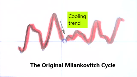
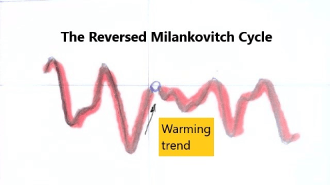
The ( Ṃ ↓ ) represents the Original Milankovitch Cycle grapheme.  And the ( Ẇ ↑ ) represents the Reversed Milankovitch Cycle grapheme.

( Ṃ ↓ ) – supposedly this is the Original Milankovitch Cycle. Please take notice of the dot under ( Ṃ ↓ ).  The dot’s position represents the present time, when Planet Earth is in Original Milankovitch Cycle Minima:  The Original Milankovitch Cycle shows a cooling trend.

( Ẇ ↑ ) The Reversed Milankovitch Cycle shows a warming trend.

Milankovitch had to reverse his cycle to match the instrumental data. But he didn’t have time.  It was a critical mistake in Milankovitch’s assumptions.  Now it is time for us to make the necessary correction. 100 years have passed, Milankovitch agrees, if it is necessary, for us to make a correction.

When comparing with the Perihelion point, which is at January 2, the solar irradiance Earth receives now is 7% less. As a result we have at the North Hemisphere much cooler summers and much warmer winters.  In 10.000 (ten thousand) years from now, Earth’s axis will be pointing at star Vega, instead of Polaris at which it points now. So in 10.000 years the Winter Solstice will occur when Earth is in Aphelion (it happens now with Earth in Perihelion).

As a result in 10.000 years we would have at the North Hemisphere much warmer summers and much cooler winters. A shift of 7% in the Hemispheres’ insolation intensity will happen.  Instead of the Southern Hemisphere (as it happens now) with its vast oceans accumulative capacity… there would be a +7% stronger insolation on the North Hemisphere’s plethora of continental areas.

We know continents do not accumulate heat so much effectively as oceans do, thus Earth will gradually cool down, until a New Ice Age commences!

As for the current warming phase – we still receive the +7% solar energy onto Southern Hemisphere’s oceans… and oceans willingly accumulate the excess solar energy…It happens so during the current Winter Solstices, when Earth is still tilted towards sun with its Southern Hemisphere’s vast oceanic waters.

The warming trend we observe now started some 6.500 years ago. It is a very slow process. The MWP ( the Medieval Warm Period ) is a confirmation of the existence of a long warming trend.  The LIA ( the Little Ice Age ) was observed as a colder atmosphere and more snowy winters. Also the glaciers were increasing.

On the other hand oceans continued accumulating heat.  It is a very long cycle. We are observing the Reversed Milankovitch Cycle culmination period. It will last about a millennia and a half and then there will be a cooling trend.

Right now Planet Earth is in an orbital forced warming trend. And these are culmination times.  The very slow warming trend will continue for about a 1,5 millennia on. Then slowly and gradually the Global Temperatures will become cooler.

US Heat and Drought Advisory June

Climatists are raising alarms about the rising temperatures and water shortages as evidence of impending doom (it’s summer and that time of year again).  So some contextual information is suitable.

First, a comparison of recent US June forecasts for temperatures.

NOAA US temp 2019 2021

And then for the same years, precipitation forecasts.

NOAA US rain 2019 2021

Finally, a reminder of how unrelated CO2 is to all of this.

us-wet-dry-co2rev-1

giss-gmt-to-2018-w-co2

Solar Cycles Chaotic

screenshot-2020-02-25-at-08.38.39-6a4eb07-e1582620697162

A recent study published at Science Daily The sun’s clock by Helmholtz-Zentrum Dresden-Rossendor Excerpts in italics with my bolds

Not only the 11-year cycle, but also all other periodic solar activity fluctuations can be clocked by planetary attractive forces. With new model calculations, they are proposing a comprehensive explanation of known sun cycles for the first time. They also reveal the longest fluctuations in activity over thousands of years as a chaotic process.

Not only the very concise 11-year cycle, but also all other periodic solar activity fluctuations can be clocked by planetary attractive forces. This is the conclusion drawn by Dr. Frank Stefani and his colleagues from the Institute of Fluid Dynamics at the Helmholtz-Zentrum Dresden-Rossendorf (HZDR) and from the Institute of Continuous Media Mechanics in Perm, Russia. With new model calculations, they are proposing a comprehensive explanation of all important known sun cycles for the first time. They also reveal the longest fluctuations in activity over thousands of years as a chaotic process. Despite the planetary timing of short and medium cycles, long-term forecasts of solar activity thus become impossible, as the researchers in the scientific journal Solar Physics assert.

Solar physicists around the world have long been searching for satisfactory explanations for the sun’s many cyclical, overlapping activity fluctuations. In addition to the most famous, approximately 11-year “Schwabe cycle,” the sun also exhibits longer fluctuations, ranging from hundreds to thousands of years. It follows, for example, the “Gleissberg cycle” (about 85 years), the “Suess-de Vries cycle” (about 200 years) and the quasi-cycle of “Bond events” (about 1500 years), each named after their discoverers. It is undisputed that the solar magnetic field controls these activity fluctuations.

Explanations and models in expert circles partly diverge widely as to why the magnetic field changes at all. Is the sun controlled externally or does the reason for the many cycles lie in special peculiarities of the solar dynamo itself? HZDR researcher Frank Stefani and his colleagues have been searching for answers for years — mainly to the very controversial question as to whether the planets play a role in solar activity.

Rosette-shaped movement of the sun can produce a 193-year cycle

The researchers have most recently taken a closer look at the sun’s orbital movement. The sun does not remain fixed at the center of the solar system: It performs a kind of dance in the common gravitational field with the massive planets Jupiter and Saturn — at a rate of 19.86 years. We know from the Earth that spinning around in its orbit triggers small motions in the Earth’s liquid core. Something similar also occurs within the sun, but this has so far been neglected with regard to its magnetic field.

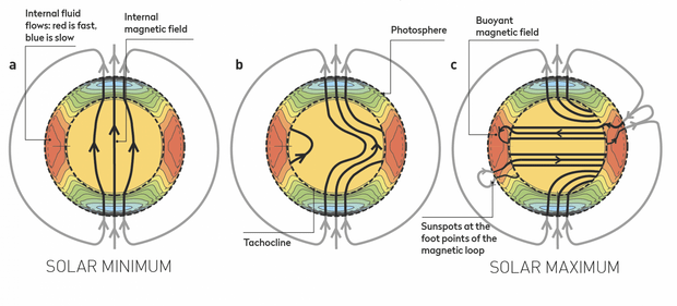
The researchers came up with the idea that part of the sun’s angular orbital momentum could be transferred to its rotation and thus affect the internal dynamo process that produces the solar magnetic field. Such coupling would be sufficient to change the extremely sensitive magnetic storage capacity of the tachocline, a transition region between different types of energy transport in the sun’s interior. “The coiled magnetic fields could then more easily snap to the sun’s surface,” says Stefani.

The researchers integrated one such rhythmic perturbation of the tachocline into their previous model calculations of a typical solar dynamo, and they were thus able to reproduce several cyclical phenomena that were known from observations. What was most remarkable was that, in addition to the 11.07-year Schwabe cycle they had already modeled in previous work, the strength of the magnetic field now also changed at a rate of 193 years — this could be the sun’s Suess-de Vries cycle, which from observations has been reported to be 180 to 230 years. Mathematically, the 193 years arise as what is known as a beat period between the 19.86-year cycle and the twofold Schwabe cycle, also called the Hale cycle. The Suess-de Vries cycle would thus be the result of a combination of two external “clocks”: the planets’ tidal forces and the sun’s own movement in the solar system’s gravitational field.

Planets as a metronome

For the 11.07-year cycle, Stefani and his researchers had previously found strong statistical evidence that it must follow an external clock. They linked this “clock” to the tidal forces of the planets Venus, Earth and Jupiter. Their effect is greatest when the planets are aligned: a constellation that occurs every 11.07 years. As for the 193-year cycle, a sensitive physical effect was also decisive here in order to trigger a sufficient effect of the weak tidal forces of the planets on the solar dynamo.

After initial skepticism toward the planetary hypothesis, Stefani now assumes that these connections are not coincidental. “If the sun was playing a trick on us here, then it would be with incredible perfection. Or, in fact, we have a first inkling of a complete picture of the short and long solar activity cycles.” In fact, the current results also retroactively reaffirm that the 11-year cycle must be a timed process. Otherwise, the occurrence of a beat period would be mathematically impossible.

Tipping into chaos: 1000-2000-year collapses are not more accurately predictable

In addition to the rather shorter activity cycles, the sun also exhibits long-term trends in the thousand-year range. These are characterized by prolonged drops in activity, known as “minima,” such as the most recent “Maunder Minimum,” which occurred between 1645 and 1715 during the “Little Ice Age.” By statistically analyzing the observed minima, the researchers could show that these are not cyclical processes, but that their occurrence at intervals of approximately one to two thousand years follows a mathematical random process.

solar-cycle-25-nasa-full

To verify this in a model, the researchers expanded their solar dynamo simulations to a longer period of 30,000 years. In fact, in addition to the shorter cycles, there were irregular, sudden drops in magnetic activity every 1000 to 2000 years. “We see in our simulations how a north-south asymmetry forms, which eventually becomes too strong and goes out of sync until everything collapses. The system tips into chaos and then takes a while to get back into sync again,” says Stefani. But this result also means that very long-term solar activity forecasts — for example, to determine influence on climate developments — are almost impossible.

Background from previous post Climate Chaos

Foucault’s pendulum in the Panthéon, Paris

h/t tom0mason for inspiring this post, including his comment below

The Pendulum is Settled Science

I attended North Phoenix High School (Go Mustangs!) where students took their required physics class from a wild and crazy guy. Decades later alumni who don’t remember his name still reminisce about “the crazy science teacher with the bowling ball.”

To demonstrate the law of conservation of energy, he required each and every student to stand on a ladder in one corner of the classroom. Attached to a hook in the center of the rather high ceiling was a rope with a bowling ball on the other end. The student held the ball to his/her nose and then released it, being careful to hold still afterwards.

The 16 pound ball traveled majestically diagonally across the room and equally impressively returned along the same path. The proof of concept was established when the ball stopped before hitting your nose (though not by much).  In those days we learned to trust science and didn’t need to go out marching to signal some abstract virtue.

The equations for pendulums are centuries old and can predict the position of the ball at any point in time based on the mass of the object, length of the rope and starting position.

Pictured above is the currently operating Foucault pendulum that exactly follows these equations. While it had long been known that the Earth rotates, the introduction of the Foucault pendulum in 1851 was the first simple proof of the rotation in an easy-to-see experiment. Today, Foucault pendulums are popular displays in science museums and universities.

What About the Double Pendulum?

Trajectories of a double pendulum

Just today a comment by tom0mason at alerted me to the science demonstrated by the double compound pendulum, that is, a second pendulum attached to the ball of the first one. It consists entirely of two simple objects functioning as pendulums, only now each is influenced by the behavior of the other.

Lo and behold, you observe that a double pendulum in motion produces chaotic behavior. In a remarkable achievement, complex equations have been developed that can and do predict the positions of the two balls over time, so in fact the movements are not truly chaotic, but with considerable effort can be determined. The equations and descriptions are at Wikipedia Double Pendulum

Long exposure of double pendulum exhibiting chaotic motion (tracked with an LED)

But here is the kicker, as described in tomomason’s comment:

If you arrive to observe the double pendulum at an arbitrary time after the motion has started from an unknown condition (unknown height, initial force, etc) you will be very taxed mathematically to predict where in space the pendulum will move to next, on a second to second basis. Indeed it would take considerable time and many iterative calculations (preferably on a super-computer) to be able to perform this feat. And all this on a very basic system of known elementary mechanics.

And What about the Climate?

This is a simple example of chaotic motion and its unpredictability. How predictable is our climate with so many variables and feedbacks, some known some unknown? Consider that this planet’s weather/climate system is chaotic in nature with many thousands (millions?) of loosely coupled variables and dependencies, and many of these variables have very complex feedback features within them.

Hurricane Gladys, photographed from orbit by Apollo 7 in 1968 (Photo: NASA)

What happens in a complex system of 10 double pendulums?

Summary

To quote the IPCC:

The climate system is a coupled non-linear chaotic system, and therefore the long-term prediction of future climate states is not possible. Rather the focus must be upon the prediction of the probability distribution of the system’s future possible states by the generation of ensembles of model solutions.

A recent National Review article draws the implications:
The range of predicted future warming is enormous — apocalyptism is unwarranted.

But as the IPCC emphasizes, the range for future projections remains enormous. The central question is “climate sensitivity” — the amount of warming that accompanies a doubling of carbon dioxide in the atmosphere. As of its Fifth Assessment Report in 2013, the IPCC could estimate only that this sensitivity is somewhere between 1.5 and 4.5°C. Nor is science narrowing that range. The 2013 assessment actually widened it on the low end, from a 2.0–4.5°C range in the prior assessment. And remember, for any specific level of warming, forecasts vary widely on the subsequent environmental and economic implications.

For now, though, navigating the climate debate will require translating the phrase “climate denier” to mean “anyone unsympathetic to the most aggressive activists’ claims.” This apparently includes anyone who acknowledges meaningful uncertainty in climate models, adopts a less-than-catastrophic outlook about the consequences of future warming, or opposes any facet of the activist policy agenda. The activists will be identifiable as the small group continuing to shout “Denier!” The “deniers” will be identifiable as everyone else.

Update May 2

Esteemed climate scientist Richard Lindzen ends a very fine recent presentation (here) with this description of the climate system:

I haven’t spent much time on the details of the science, but there is one thing that should spark skepticism in any intelligent reader. The system we are looking at consists in two turbulent fluids interacting with each other. They are on a rotating planet that is differentially heated by the sun. A vital constituent of the atmospheric component is water in the liquid, solid and vapor phases, and the changes in phase have vast energetic ramifications. The energy budget of this system involves the absorption and reemission of about 200 watts per square meter. Doubling CO2 involves a 2% perturbation to this budget. So do minor changes in clouds and other features, and such changes are common. In this complex multifactor system, what is the likelihood of the climate (which, itself, consists in many variables and not just globally averaged temperature anomaly) is controlled by this 2% perturbation in a single variable? Believing this is pretty close to believing in magic. Instead, you are told that it is believing in ‘science.’ Such a claim should be a tip-off that something is amiss. After all, science is a mode of inquiry rather than a belief structure.

Flow Diagram for Climate Modeling, Showing Feedback Loops