Climate Answers Blowing in the Wind
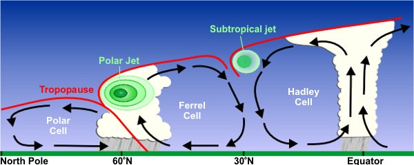
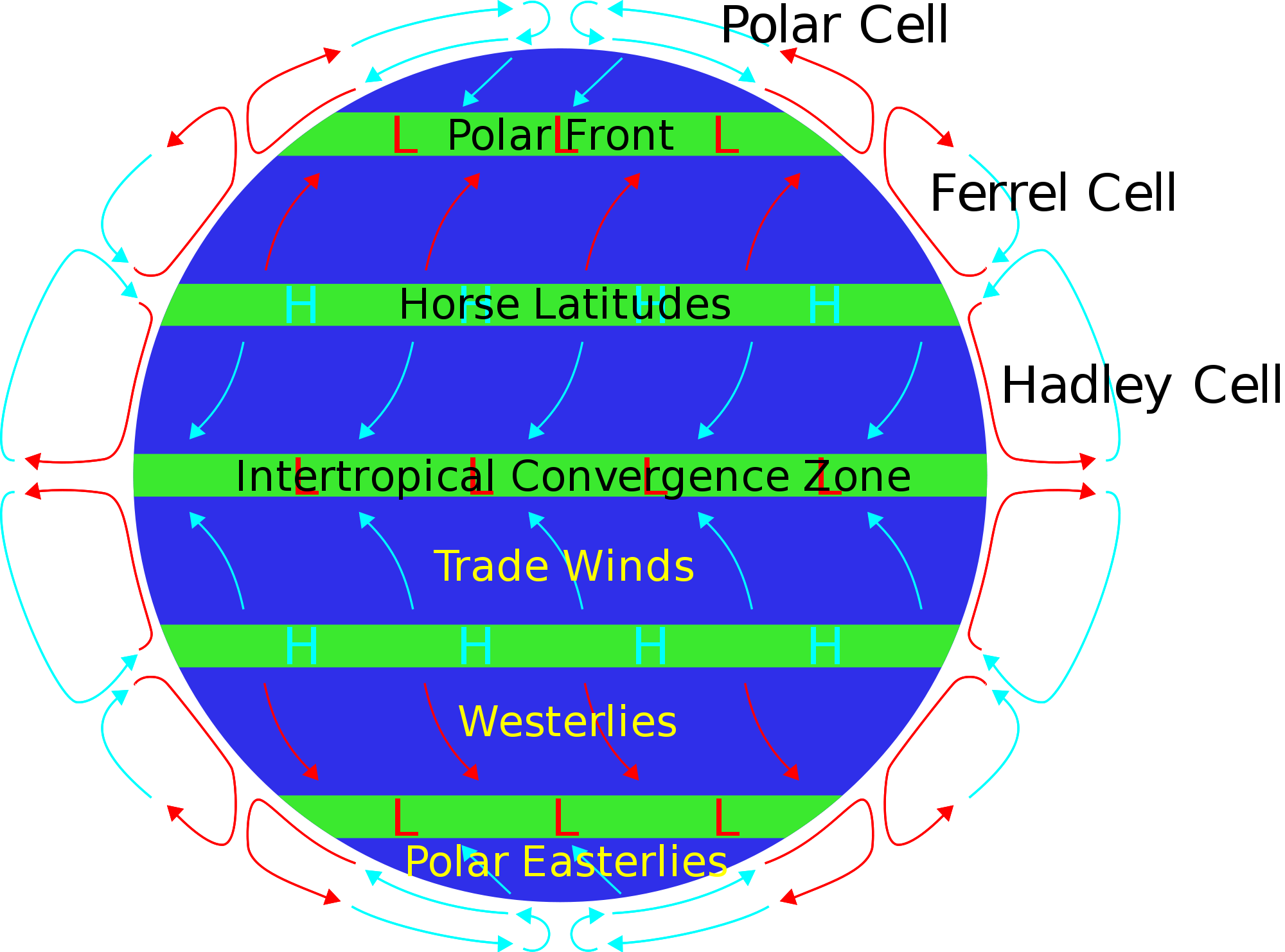
The subtropical jet streams are weaker and higher in the atmosphere at 10-16 kilometers above sea level. Jet streams wander laterally in quite dramatic waves and can exhibit huge changes in altitude. Breaks in the tropopause at the Polar, Hadley and Ferrel circulation cells cause the streams to form. The combination of circulation and Coriolis forces acting on the cell masses drive the phenomenon. The Polar jet, being at a lower altitude, strongly affects weather and aviation. It is most often found between the latitudes of 30 degrees and 60 degrees, while you can find the subtropical jets at 30 degrees. A jet stream is generally a few hundred kilometers wide and only about 5 kilometers high.

Fundamental questions and unknowns concerning natural climate change are presented in this 2007 essay Challenges to Our Understanding of the General Circulation: Abrupt Climate Change by Richard Seager and David S. Battisti. Excerpts in italics with my bolds.

The abrupt climate changes that occurred during the last glaciation and deglaciation are mind boggling both in terms of rapidity and magnitude. That winters in the British Isles could switch between mild, wet ones very similar to today and ones in which winter temperatures dropped to as much as 20◦C below freezing, and do so in years to decades, is simply astounding. No state-of-the-art climate model, of the kind used to project future climate change within the Intergovernmental Panel on Climate Change process, has ever produced a climate change like this.

The problem for dynamicists working in this area is that the period of instrumental observationsand model simulations of that period, do not provide even a hint that drastic climate reorganizations can occur.  Our understanding of the general circulation is based fundamentally on this period or, more correctly, on the last 50 years of it, a time of gradual climate change or, at best, more rapid changes of modest amplitude. So it is not surprising that our encyclopedia of knowledge of the general circulations contains many ideas of negative feedbacks between circulation features that may help explain climate variability but also stabilize the climate (Bjerknes 1964; Hazeleger et al. 2005; Shaffrey and Sutton 2004). The modern period has not been propitious for studying how the climate can run away to a new state. Because of this, our understanding has to be limited

The normal explanation of how such changes occurred is that deepwater formation in the Nordic Seas abruptly ceased or resumed forcing a change in ocean heat flux convergence and changes in sea ice. However, coupled GCMs only produce such rapid cessations in response to unrealistically large freshwater forcing and have not so far produced a rapid resumption.

The discussions of the spatial extent of abrupt climate changes in glacial times and during the last deglaciation should make it clear that the causes must be found in changes in the general circulations of the global, as opposed to regional, atmosphere and ocean circulation. The idea that the THC changes and directly impacts a small area of the globe, and that somehow most of the rest of the world piggy-backs along in a rather systematic and reliable way seems dubious.

Thus the problems posed by abrupt change in the North Atlantic region are:
1. How could sea ice extend so far south in winter during the stadials?
2. How, during the spring and summer of stadials, can there be such an enormous influx of heat as to melt the ice and warm the water below by close to 10◦C? If 50 m of water needs to be warmed up by this much in four months, it would take an average net surface heat flux of 150 Wm−2, more than twice the current average between early spring and midsummer and more than can be accounted for by any increase in summer solar irradiance (as during the Younger Dryas).
3. How can this stadial state of drastic seasonality abruptly shift into one similar to that of today with a highly maritime climate in western Europe? Remember that both states can exist in the presence of large ice sheets over North America and Scandinavia.

In thinking of ways to reduce the winter convergence of heat into the mid and high-latitude North Atlantic, we might begin with the storm tracks and mean atmosphere circulation. The Atlantic storm track and jet stream have a clear southwest-to-northeast trajectory, whereas the Pacific ones are more zonal over most of their longitudinal reach (Hoskins and Valdes 1990). If the Atlantic storm track and jet could be induced to take a more zonal track, akin to its Pacific cousin, the North Atlantic would cool.

Here we have argued that the abrupt changes must involve more than changes in the North Atlantic Ocean circulation. In particular it is argued that the degree of winter cooling around the North Atlantic must be caused by a substantial change in the atmospheric circulation involving a great reduction of atmospheric heat transport into the region. Such a change could, possibly, be due to a switch to a regime of nearly zonal wind flow across the Atlantic, denying western Europe the warm advection within stationary waves that is the fundamental reason for why Europe’s winters are currently so mild. Such a change in wind regime would, presumably, also cause a change in the North Atlantic Ocean circulation as the poleward flow of warm, salty waters from the tropics into the Nordic Seas is diverted south by the change in wind stress curl. This would impact the location and strength of deep water formation and allow sea ice to expand south.

The North Atlantic Oscillation (NAO) is is a largely atmospheric mode from fluctuations in the difference of atmospheric pressure at sea level (SLP) between the Icelandic low and the Azores high. Through fluctuations in the strength of the Icelandic low and the Azores high, it controls the strength and direction of westerly winds and location of storm tracks across the North Atlantic. It is part of the Arctic oscillation, and varies over time with no particular periodicity. Wikipedia

Recent Wind Research

A decade later we have further insight into the role of winds in climate change by means  of a paper discussed in this Futurity article Wind shifts may explain Europe’s ‘weird’ winters  Excerpts in italics with my bolds.

In the mid-1990s, scientists assembled the first century-long record of North Atlantic sea surface temperatures and quickly discovered a cycle of heating and cooling at the surface of the ocean. Each of these phases lasted for decades, even as temperatures warmed overall during the course of the century. Since this discovery, these fluctuations in ocean temperature have been linked to all manner of Northern Hemisphere climate disturbances, from Sahel drought to North Atlantic hurricanes.

Research also linked European climate variability to the temperature swings of its neighboring ocean in the spring, summer, and fall. Surprisingly, however, no imprint of the ocean’s variability could be found in Western Europe’s wintertime temperature record. This absence was especially puzzling in light of the fact that Europe’s mild winters are a direct consequence of its enviable location downwind of the North Atlantic.

Now, a study by researchers at McGill University and the University of Rhode Island suggests the answer to this puzzle lies in the winds themselves. The fluctuations in ocean temperature are accompanied by shifts in the winds. These wind shifts mean that air arrives in Western Europe via very different pathways in decades when the surface of the North Atlantic is warm, compared to decades when it is cool.
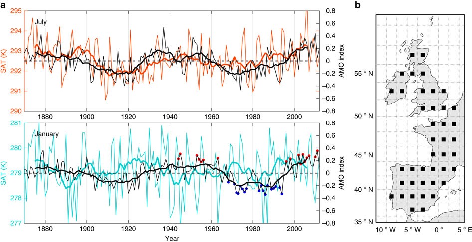
(a) Time series of the linearly detrended North Atlantic SST (black lines, referred to as the AMO index) and SAT averaged over western Europe ([36N 60N] × [10W 3E]; shown in coloured lines) in July (top panel) and January (bottom panel). Bold lines show 10-year running means. The correlation coefficient between the 10-year running mean of the detrended SAT and AMO index is 0.61 in July (statistically significant at 10% confidence level even after accounting for the reduced effective degrees of freedom due to autocorrelation of the time series) and −0.02 in January; these correlations are insensitive to the averaging region chosen for western Europe. The red circles on January plot indicate the AMO-positive years chosen for the composite analysis, whereas the blue circles indicate the AMO-negative years chosen. (b) Study region encompassing western Europe ([36N 60N] × [10W 3E]) and locations for the backtracked Lagrangian particle release (black squares).

The researchers studied the winds and their interaction with the ocean in a recently developed reconstruction of 20th-century climate. Their main approach was to launch virtual particles into the winds, and trace their journey for ten key days leading up to their arrival in Western Europe. They repeated this procedure using the wind field for each winter of the last 72 years, a period for which the winds of the North Atlantic have already been carefully documented and validated.

The new research reveals that in decades in which North Atlantic sea surface temperatures are elevated, winds deliver air to Europe disproportionately from the north.

In contrast, in decades of coolest sea surface temperature, swifter winds extract more heat from the western and central Atlantic before arriving in Europe. The researchers suggest the distinct atmospheric pathways hide the ocean oscillation from Europe in winter.

“It is often presumed that the cooler North Atlantic will quickly lead to cooling in Europe, or at least a slowdown in its rate of warming,” says Ayako Yamamoto, a PhD student at McGill University and lead author of the study. “But our research suggests that the dynamics of the atmosphere might stop this relative cooling from showing up in Europe in winter in the decades following an Atlantic cooling.”

The complete paper is The absence of an Atlantic imprint on the multidecadal variability of wintertime European temperature by Ayako Yamamoto & Jaime B. Palter Nature Communications (2016). Excerpts in italics with my bolds.
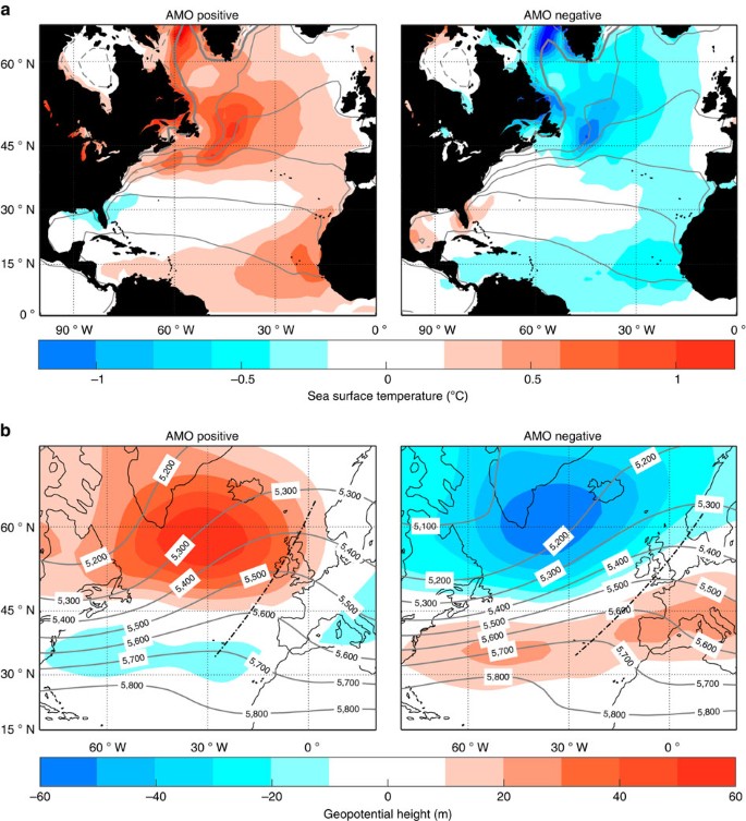
Figure 2: The spatial pattern of the AMO index and its relationship with the atmospheric flow in January. Composite maps of (a) sea surface temperature (SST) field and (b) 500 hPa geopotential height field (Z500) for AMO anomalously positive years (left panel) and negative years (right panel). The January mean field is shown in contours, and its departure from the 72-year climatology is represented by colour shading. The thick grey contour line in a denotes 0 °C, whereas thin (dashed) lines denote positive (negative) SST every 5 °C. The black dashed lines in b are drawn through the local maxima of the geopotential height field at each latitude, which is the point where the wind changes direction from south–westerly to north–westerly.

The large-scale atmospheric flow varies with the AMO index (Fig. 2b). The difference in the 500-hPa geopotential height (Z500) field, which is analogous to streamlines, shows that the direction of winds arriving in western Europe changes between the two AMO phases: winds are more northerly during the anomalous AMO-positive years, whereas they are more zonal during the AMO-negative years (Fig. 2b). The more tightly spaced isohypses during the AMO-negative years indicate a swifter flow relative to the AMO-positive years. Accordingly, the AMO-negative years see an elongated and more zonal January storm track (Supplementary Fig. 1), which is consistent with results from a free-running climate model7. Composite Z500 maps constructed with more complete sampling of the longer decadal periods associated with the AMO show similar, albeit weaker, anomaly patterns (Supplementary Fig. 2a).

In winter in the North Atlantic, SST is almost always warmer than the surface air temperature (SAT), so the ocean loses heat rapidly to the atmosphere over the entirety of the basin (that is, positive fluxes in our convention; Fig. 3b and Supplementary Fig. 3b). The fluxes over the warm Gulf Stream and its North Atlantic Current extension are generally a factor of five higher than found elsewhere. However, a view of the fluxes weighted by the fraction of time the particles spend in each location on their journey to western Europe (Fig. 3c and Supplementary Fig. 3c) suggests a reduced role of these strong flux regions in establishing western European wintertime temperature.

The difference in the number density of the particle positions between the composite AMO periods (Fig. 3d) shows a significant distinction in the preferred pathways, with the statistical significance increasing when results are separated by particles launched from northern and southern sub-regions of western Europe (Supplementary Fig. 3d). In the AMO-positive years, particles spend more of their 10-day trajectory recirculating locally to the southwest of Iceland. During the AMO-negative years, the pathways are anomalously long, and a greater number of trajectories originate from North America and the Arctic, before transiting over the Labrador Sea and mid-latitude North Atlantic.

The strengthening and lengthening of the storm track in sync with anomalously cooler North Atlantic SSTs has important implications for future climate. Given that decadal variability in North Atlantic SSTs may be driven partly by fluctuations in the strength of the AMOC10,11,12, our result suggests the possibility of a stabilizing feedback for ocean circulation: Cooler SSTs associated with a sluggish AMOC is linked with an atmospheric adjustment that enhances turbulent heat fluxes over oceanic convective regions in winter. These larger fluxes could possibly reinvigorate convection, deep water formation and the AMOC. Moreover, the observed link of the atmospheric circulation with the cool SST anomalies of the late 1970s to early 1990s is much like the predicted change of the storm track in response to a decline of the AMOC under global warming36. A weakened AMOC has long been thought to cause anomalous cooling in western Europe via a decline in oceanic heat transport and associated atmospheric feedbacks21. However, the changes we describe here in atmospheric Lagrangian trajectories and the heat fluxes along them could provide a mechanism that reduces the magnitude of European wintertime cooling on decadal time scales, even as they might stabilize the oceanic circulation.

The answer is blowin’ in the wind.  Bob Dylan


Concurrent Warming and Cooling

Rannoch Moor and Glencoe Landscape. Scotland Images by Nigel For is a photograph I by Nigel Forster which was uploaded on May 30th, 2019.

This post highlights recent interesting findings regarding past climate change in NH, Scotland in particular. The purpose of the research was to better understand how glaciers could be retreating during the Younger Dryas Stadia (YDS), one of the coldest periods in our Holocene epoch.

The lead researcher is Gordon Bromley, and the field work was done on site of the last ice fields on the highlands of Scotland. 14C dating was used to estimate time of glacial events such as vegetation colonizing these places. Bromley explains in an article Shells found in Scotland rewrite our understanding of climate change at siliconrepublic. Excerpts in italics with my bolds.

By analysing ancient shells found in Scotland, the team’s data challenges the idea that the period was an abrupt return to an ice age climate in the North Atlantic, by showing that the last glaciers there were actually decaying rapidly during that period.

The shells were found in glacial deposits, and one in particular was dated as being the first organic matter to colonise the newly ice-free landscape, helping to provide a minimum age for the glacial advance. While all of these shell species are still in existence in the North Atlantic, many are extinct in Scotland, where ocean temperatures are too warm.

This means that although winters in Britain and Ireland were extremely cold, summers were a lot warmer than previously thought, more in line with the seasonal climates of central Europe.

“There’s a lot of geologic evidence of these former glaciers, including deposits of rubble bulldozed up by the ice, but their age has not been well established,” said Dr Gordon Bromley, lead author of the study, from NUI Galway’s School of Geography and Archaeology.

“It has largely been assumed that these glaciers existed during the cold Younger Dryas period, since other climate records give the impression that it was a cold time.”

He continued: “This finding is controversial and, if we are correct, it helps rewrite our understanding of how abrupt climate change impacts our maritime region, both in the past and potentially into the future.”

The recent report is Interstadial Rise and Younger Dryas Demise of Scotland’s Last Ice Fields
G. Bromley A. Putnam H. Borns Jr T. Lowell T. Sandford D. Barrell  First published: 26 April 2018.(my bolds)

Abstract

Establishing the atmospheric expression of abrupt climate change during the last glacial termination is key to understanding driving mechanisms. In this paper, we present a new 14C chronology of glacier behavior during late‐glacial time from the Scottish Highlands, located close to the overturning region of the North Atlantic Ocean. Our results indicate that the last pulse of glaciation culminated between ~12.8 and ~12.6 ka, during the earliest part of the Younger Dryas stadial and as much as a millennium earlier than several recent estimates. Comparison of our results with existing minimum‐limiting 14C data also suggests that the subsequent deglaciation of Scotland was rapid and occurred during full stadial conditions in the North Atlantic. We attribute this pattern of ice recession to enhanced summertime melting, despite severely cool winters, and propose that relatively warm summers are a fundamental characteristic of North Atlantic stadials.

Plain Language Summary

Geologic data reveal that Earth is capable of abrupt, high‐magnitude changes in both temperature and precipitation that can occur well within a human lifespan. Exactly what causes these potentially catastrophic climate‐change events, however, and their likelihood in the near future, remains frustratingly unclear due to uncertainty about how they are manifested on land and in the oceans. Our study sheds new light on the terrestrial impact of so‐called “stadial” events in the North Atlantic region, a key area in abrupt climate change. We reconstructed the behavior of Scotland’s last glaciers, which served as natural thermometers, to explore past changes in summertime temperature. Stadials have long been associated with extreme cooling of the North Atlantic and adjacent Europe and the most recent, the Younger Dryas stadial, is commonly invoked as an example of what might happen due to anthropogenic global warming. In contrast, our new glacial chronology suggests that the Younger Dryas was instead characterized by glacier retreat, which is indicative of climate warming. This finding is important because, rather than being defined by severe year‐round cooling, it indicates that abrupt climate change is instead characterized by extreme seasonality in the North Atlantic region, with cold winters yet anomalously warm summers.

The complete report is behind a paywall, but a 2014 paper by Bromley discusses the evidence and analysis in reaching these conclusions. Younger Dryas deglaciation of Scotland driven by warming summers  Excerpts with my bolds.

Significance: As a principal component of global heat transport, the North Atlantic Ocean also is susceptible to rapid disruptions of meridional overturning circulation and thus widely invoked as a cause of abrupt climate variability in the Northern Hemisphere. We assess the impact of one such North Atlantic cold event—the Younger Dryas Stadial—on an adjacent ice mass and show that, rather than instigating a return to glacial conditions, this abrupt climate event was characterized by deglaciation. We suggest this pattern indicates summertime warming during the Younger Dryas, potentially as a function of enhanced seasonality in the North Atlantic.

Surface temperatures range from -30C to +30C

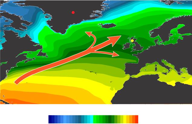
Fig. 1. Surface temperature and heat transport in the North Atlantic Ocean.  The relatively mild European climate is sustained by warm sea-surface temperatures and prevailing southwesterly airflow in the North Atlantic Ocean (NAO), with this ameliorating effect being strongest in maritime regions such as Scotland. Mean annual temperature (1979 to present) at 2 m above surface (image obtained using University of Maine Climate Reanalyzer, http://www.cci-reanalyzer.org). Locations of Rannoch Moor and the GISP2 ice core are indicated.

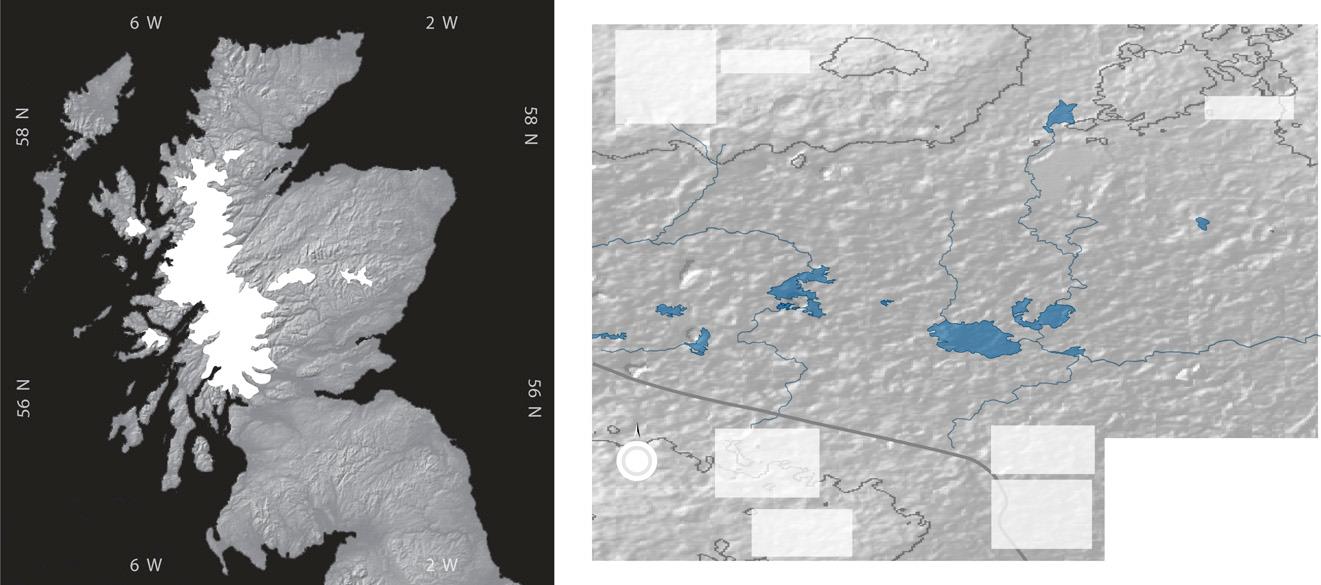
Thus the Scottish glacial record is ideal for reconstructing late glacial variability in North Atlantic temperature (Fig. 1). The last glacier resurgence in Scotland—the “Loch Lomond Advance” (LLA)—culminated in a ∼9,500-km2 ice cap centered over Rannoch Moor (Fig. 2A) and surrounded by smaller ice fields and cirque glaciers.

Fig. 2. Extent of the LLA ice cap in Scotland and glacial geomorphology of western Rannoch Moor. (A) Maximum extent of the ∼9,500 km2 LLA ice cap and larger satellite ice masses, indicating the central location of Rannoch Moor. Nunataks are not shown. (B) Glacial-geomorphic map of western Rannoch Moor. Distinct moraine ridges mark the northward active retreat of the glacier margin (indicated by arrow) across this sector of the moor, whereas chaotic moraines near Lochan Meall a’ Phuill (LMP) mark final stagnation of ice. Core sites are shown, including those (K1–K3) of previous investigations (14, 15).

When did the LLA itself occur? We consider two possible resolutions to the paradox of deglaciation during the YDS. First, declining precipitation over Scotland due to gradually increasing North Atlantic sea-ice extent has been invoked to explain the reported shrinkage of glaciers in the latter half of the YDS (18). However, this course of events conflicts with recent data depicting rapid, widespread imposition of winter sea-ice cover at the onset of the YDS (9), rather than progressive expansion throughout the stadial.

Loch Lomond

Furthermore, considering the gradual active retreat of LLA glaciers indicated by the geomorphic record, our chronology suggests that deglaciation began considerably earlier than the mid-YDS, when precipitation reportedly began to decline (18). Finally, our cores contain lacustrine sediments deposited throughout the latter part of the YDS, indicating that the water table was not substantially different from that of today. Indeed, some reconstructions suggest enhanced YDS precipitation in Scotland (24, 25), which is inconsistent with the explanation that precipitation starvation drove deglaciation (26).

We prefer an alternative scenario in which glacier recession was driven by summertime warming and snowline rise. We suggest that amplified seasonality, driven by greatly expanded winter sea ice, resulted in a relatively continental YDS climate for western Europe, both in winter and in summer. Although sea-ice formation prevented ocean–atmosphere heat transfer during the winter months (10), summertime melting of sea ice would have imposed an extensive freshwater cap on the ocean surface (27), resulting in a buoyancy-stratified North Atlantic. In the absence of deep vertical mixing, summertime heating would be concentrated at the ocean surface, thereby increasing both North Atlantic summer sea-surface temperatures (SSTs) and downwind air temperatures. Such a scenario is analogous to modern conditions in the Sea of Okhotsk (28) and the North Pacific Ocean (29), where buoyancy stratification maintains considerable seasonal contrasts in SSTs. Indeed, Haug et al. (30) reported higher summer SSTs in the North Pacific following the onset of stratification than previously under destratified conditions, despite the growing presence of northern ice sheets and an overall reduction in annual SST. A similar pattern is evident in a new SST record from the northeastern North Atlantic, which shows higher summer temperatures during stadial periods (e.g., Heinrich stadials 1 and 2) than during interstadials on account of amplified seasonality (30).

Our interpretation of the Rannoch Moor data, involving the summer (winter) heating (cooling) effects of a shallow North Atlantic mixed layer, reconciles full stadial conditions in the North Atlantic with YDS deglaciation in Scotland. This scenario might also account for the absence of YDS-age moraines at several higher-latitude locations (12, 36–38) and for evidence of mild summer temperatures in southern Greenland (11). Crucially, our chronology challenges the traditional view of renewed glaciation in the Northern Hemisphere during the YDS, particularly in the circum-North Atlantic, and highlights our as yet incomplete understanding of abrupt climate change.

Summary

Several things are illuminated by this study. For one thing, glaciers grow or recede because of multiple factors, not just air temperature. The study noted that glaciers require precipitation (snow) in order to grow, but also melt under warmer conditions. For background on the complexities of glacier dynamics see Glaciermania

Also, paleoclimatology relies on temperature proxies who respond to changes over multicentennial scales at best. C14 brings higher resolution to the table.

Finally, it is interesting to consider climate changing with respect to seasonality.  Bromley et al. observe that during Younger Dryas, Scotland shifted from a moderate maritime climate to one with more seasonal extremes like that of inland continental regions. In that light, what should we expect from cooler SSTs in the North Atlantic?

Note also that our modern warming period has been marked by the opposite pattern. Many NH temperature records show slight summer cooling along with somewhat stronger warming in winter, the net being the modest (fearful?) warming in estimates of global annual temperatures.

It seems that climate shifts are still events we see through a glass darkly.


Six Cloud Types Tell You the Weather

This informative post comes from Hannah Christensen Six clouds you should know about – and what they can reveal about the weather March 23, 2018 at phys.org. Text and images from the article.

You don’t need a supercomputer to predict how the weather above your head is likely to change over the next few hours – this has been known across cultures for millennia. By keeping an eye on the skies above you, and knowing a little about how clouds form, you can predict whether rain is on the way.

And moreover, a little understanding of the physics behind cloud formation highlights the complexity of the atmosphere, and sheds some light on why predicting the weather beyond a few days is such a challenging problem.

So here are six clouds to keep an eye out for, and how they can help you understand the weather.

1. Cumulus

Clouds form when air cools to the dew point, the temperature at which the air can no longer hold all its water vapour. At this temperature, water vapour condenses to form droplets of liquid water, which we observe as a cloud. For this process to happen, we require air to be forced to rise in the atmosphere, or for moist air to come into contact with a cold surface.

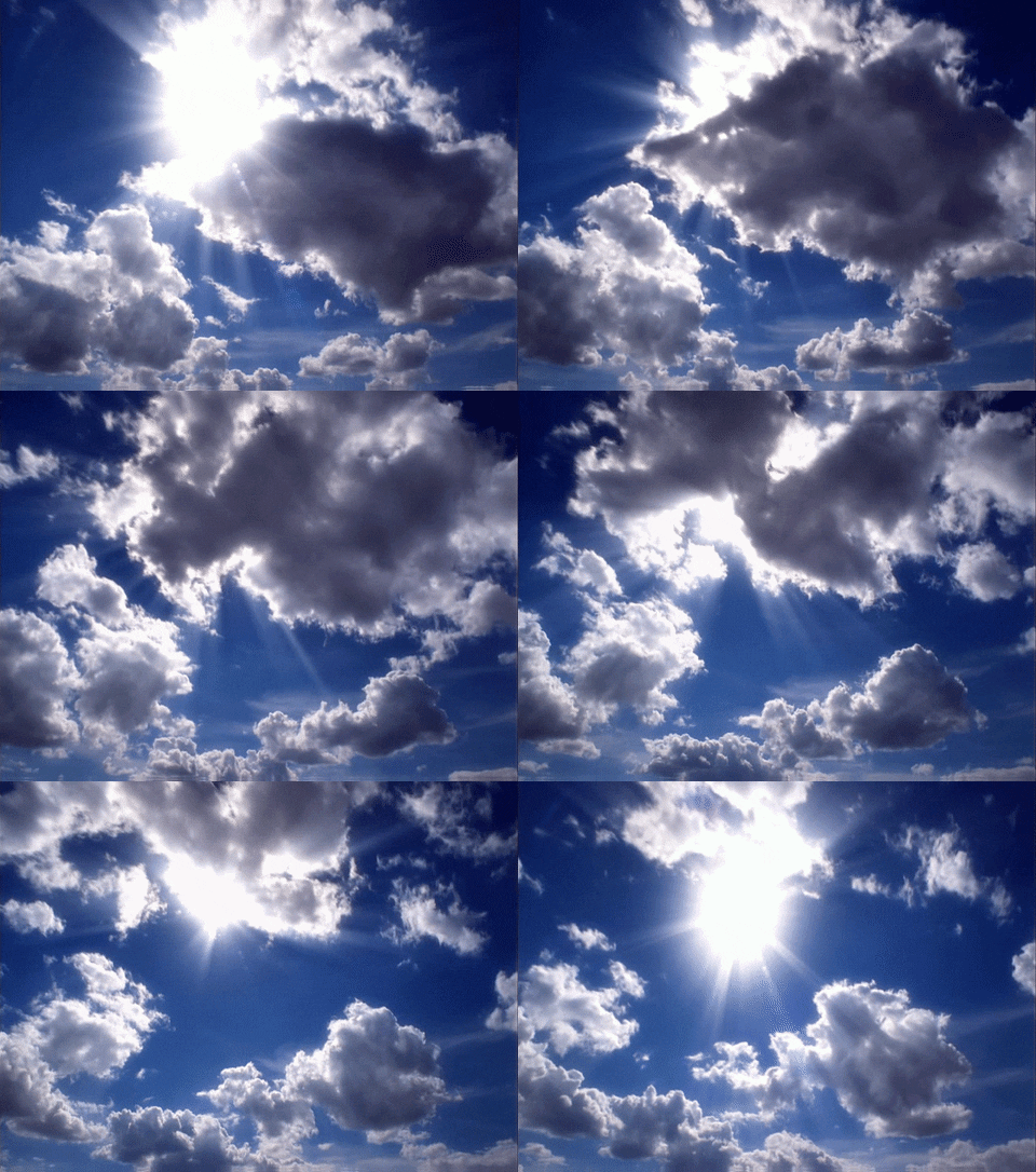
On a sunny day, the sun’s radiation heats the land, which in turn heats the air just above it. This warmed air rises by convection and forms Cumulus. These “fair weather” clouds look like cotton wool. If you look at a sky filled with cumulus, you may notice they have flat bases, which all lie at the same level. At this height, air from ground level has cooled to the dew point. Cumulus clouds do not generally rain – you’re in for fine weather.

2. Cumulonimbus

While small Cumulus do not rain, if you notice Cumulus getting larger and extending higher into the atmosphere, it’s a sign that intense rain is on the way. This is common in the summer, with morning Cumulus developing into deep Cumulonimbus (thunderstorm) clouds in the afternoon.

Near the ground, Cumulonimbus are well defined, but higher up they start to look wispy at the edges. This transition indicates that the cloud is no longer made of water droplets, but ice crystals. When gusts of wind blow water droplets outside the cloud, they rapidly evaporate in the drier environment, giving water clouds a very sharp edge. On the other hand, ice crystals carried outside the cloud do not quickly evaporate, giving a wispy appearance.

Cumulonimbus are often flat-topped. Within the Cumulonimbus, warm air rises by convection. In doing so, it gradually cools until it is the same temperature as the surrounding atmosphere. At this level, the air is no longer buoyant so cannot rise further. Instead it spreads out, forming a characteristic anvil shape.

3. Cirrus

Cirrus form very high in the atmosphere. They are wispy, being composed entirely of ice crystals falling through the atmosphere. If Cirrus are carried horizontally by winds moving at different speeds, they take a characteristic hooked shape. Only at very high altitudes or latitudes do Cirrus produce rain at ground level.

But if you notice that Cirrus begins to cover more of the sky, and gets lower and thicker, this is a good indication that a warm front is approaching. In a warm front, a warm and a cold air mass meet. The lighter warm air is forced to rise over the cold air mass, leading to cloud formation. The lowering clouds indicate that the front is drawing near, giving a period of rain in the next 12 hours.

4. Stratus

Stratus is a low continuous cloud sheet covering the sky. Stratus forms by gently rising air, or by a mild wind bringing moist air over a cold land or sea surface. Stratus cloud is thin, so while conditions may feel gloomy, rain is unlikely, and at most will be a light drizzle. Stratus is identical to fog, so if you’ve ever been walking in the mountains on a foggy day, you’ve been walking in the clouds.

5. Lenticular

Our final two cloud types will not help you predict the coming weather, but they do give a glimpse of the extraordinarily complicated motions of the atmosphere. Smooth, lens-shaped Lenticular clouds form as air is blown up and over a mountain range.

Once past the mountain, the air sinks back to its previous level. As it sinks, it warms and the cloud evaporates. But it can overshoot, in which case the air mass bobs back up allowing another Lenticular cloud to form. This can lead to a string of clouds, extending some way beyond the mountain range. The interaction of wind with mountains and other surface features is one of the many details that have to be represented in computer simulators to get accurate predictions of the weather.

6. Kelvin-Helmholtz

And lastly, my personal favourite. The Kelvin-Helmholtzcloud resembles a breaking ocean wave. When air masses at different heights move horizontally with different speeds, the situation becomes unstable. The boundary between the air masses begins to ripple, eventually forming larger waves.

Kelvin-Helmholtz clouds are rare – the only time I spotted one was over Jutland, western Denmark – because we can only see this process taking place in the atmosphere if the lower air mass contains a cloud. The cloud can then trace out the breaking waves, revealing the intricacy of the otherwise invisible motions above our heads.


Updated: Fears and Facts about Reservoirs and GHGs


A previous post explained how methane has been hyped in support of climate alarmism/activism. Now we have an additional campaign to disparage hydropower because of methane emissions from dam reservoirs. File this under “They have no shame.” Excerpts below with my bolds.

On March 5, 2018 a study was published in Environmental Research Letters Greenhouse gas emissions of hydropower in the Mekong River Basin can exceed those of fossil fuel energy sources

“The hydropower related emissions started in the Mekong in mid-1960’s when the first large reservoir was built in Thailand, and the emissions increased considerably in early 2000’s when hydropower development became more intensive. Currently the emissions are estimated to be around 15 million tonnes of CO2e per year, which is more than total emissions of all sectors in Lao PDR in year 2013,” says Dr Timo Räsänen who led the study. The GHG emissions are expected to increase when more hydropower is built. However, if construction of new reservoirs is halted, the emissions will decline slowly in time.

Another recent example of the claim is from Asia Times Global hydropower boom will add to climate change

The study, published in BioScience, looked at the carbon dioxide (CO2), methane (CH4), and nitrous oxide (N2O) emitted from 267 reservoirs across six continents. In total, the reservoirs studied have a surface area of more than 77,287 square kilometers (29,841 square miles). That’s equivalent to about a quarter of the surface area of all reservoirs in the world, which together cover 305,723 sq km – roughly the combined size of the United Kingdom and Ireland.

“The new study confirms that reservoirs are major emitters of methane, a particularly aggressive greenhouse gas,” said Kate Horner, Executive Director of International Rivers, adding that hydropower dams “can no longer be considered a clean and green source of electricity.”

In fact, methane’s effect is 86 times greater than that of CO2 when considered on this two-decade timescale. Importantly, the study found that methane is responsible for 90% of the global warming impact of reservoir emissions over 20 years.

Alarmists are Wrong about Hydropower

Now CH4 is proclaimed the primary culprit held against hydropower. As usual, there is a kernel of truth buried beneath this obsessive campaign: Flooding of biomass does result in decomposition accompanied by some release of CH4 and CO2. From HydroQuebec:  Greenhouse gas emissions and reservoirs

Impoundment of hydroelectric reservoirs induces decomposition of a small fraction of the flooded biomass (forests, peatlands and other soil types) and an increase in the aquatic wildlife and vegetation in the reservoir.

The result is higher greenhouse gas (GHG) emissions after impoundment, mainly CO2 (carbon dioxide) and a small amount of CH4 (methane).

However, these emissions are temporary and peak two to four years after the reservoir is filled.

During the ensuing decade, CO2 emissions gradually diminish and return to the levels given off by neighboring lakes and rivers.

Hydropower generation, on average, emits 50 times less GHGs than a natural gas generating station and about 70 times less than a coal-fired generating station.

The Facts about Tropical Reservoirs

Activists estimate Methane emissions from dams and reservoirs across the planet, including hydropower, are estimated to be significantly larger than previously thought, approximately equal to 1 gigaton per year.

Activists also claim that dams in boreal regions like Quebec are not the problem, but tropical reservoirs are a big threat to the climate. Contradicting that is an intensive study of Brazilian dams and reservoirsGreenhouse Gas Emissions from Reservoirs: Studying the Issue in Brazil

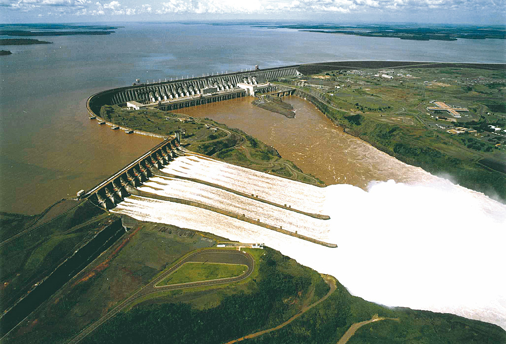
The Itaipu Dam is a hydroelectric dam on the Paraná River located on the border between Brazil and Paraguay. The name “Itaipu” was taken from an isle that existed near the construction site. In the Guarani language, Itaipu means “the sound of a stone”. The American composer Philip Glass has also written a symphonic cantata named Itaipu, in honour of the structure.

Five Conclusions from Studying Brazilian Reservoirs

1) The budget approach is essential for a proper grasp of the processes going on in reservoirs. This approach involves taking into account the ways in which the system exchanged GHGs with the atmosphere before the reservoir was flooded. Older studies measured only the emissions of GHG from the reservoir surface or, more recently, from downstream de-gassing. But without the measurement of the inputs of carbon to the system, no conclusions can be drawn from surface measurements alone.

2) When you consider the total budgets, most reservoirs acted as sinks of carbon in the short run (our measurements covered one year in each reservoir). In other words, they received more carbon than they exported to the atmosphere and to downstream.

3) Smaller reservoirs are more efficient as carbon traps than the larger ones.

4) As for the GHG impact, in order to determine it, we should add the methane (CH4) emissions to the fraction of carbon dioxide (CO2) emissions which comes from the flooded biomass and organic carbon in the flooded (terrestrial) soil. The other CO2 emissions, arising from the respiration of aquatic organisms or from the decomposition of terrestrial detritus that flows into the reservoir (including domestic sewage), are not impacts of the reservoir. From this sum, we should deduct the amount of carbon that is stored in the sediment and which will be kept there for at least the life of the reservoir (usually more than 80 years). This “stored carbon” ranges from as little as 2 percent of the total carbon output to more than 25 percent, depending on the reservoirs.

5) When we assess the GHG impacts following the guidelines just described, all of FURNAS’s reservoirs have lower emissions than the cleanest European oil plant. The worst case – Manso, which was sampled only three years after the impoundment, and therefore in a time in which the contribution from the flooded biomass was still very significant – emitted about half as much carbon dioxide equivalents (CO2 eq) as the average oil plant from the United States (CO2 eq is a metric measure used to compare the emissions from various greenhouse gases based upon their global warming potential, GWP. CO2 eq for a gas is derived by multiplying the tons of the gas by the associated GWP.) We also observed a very good correlation between GHG emissions and the age of the reservoirs. The reservoirs older than 30 years had negligible emissions, and some of them had a net absorption of CO2eq.

Keeping Methane in Perspective

Over the last 30 years, CH4 in the atmosphere increased from 1.6 ppm to 1.8 ppm, compared to CO2, presently at 400 ppm. So all the dam building over 3 decades, along with all other land use was part of a miniscule increase of a microscopic gas, 200 times smaller than the trace gas, CO2.

Background Facts on Methane and Climate Change

Methane pollution surrounding Porter Ranch, LA, ( Photo credit: Energy Efficiency Team)


The US Senate is considering an act to repeal with prejudice an Obama anti-methane regulation. The story from activist source Climate Central is
Senate Mulls ‘Kill Switch’ for Obama Methane Rule

The U.S. Senate is expected to vote soon on whether to use the Congressional Review Act to kill an Obama administration climate regulation that cuts methane emissions from oil and gas wells on federal land. The rule was designed to reduce oil and gas wells’ contribution to climate change and to stop energy companies from wasting natural gas.

The Congressional Review Act is rarely invoked. It was used this month to reverse a regulation for the first time in 16 years and it’s a particularly lethal way to kill a regulation as it would take an act of Congress to approve a similar regulation. Federal agencies cannot propose similar regulations on their own.

The Claim Against Methane

Now some Republican senators are hesitant to take this step because of claims like this one in the article:

Methane is 86 times more potent as a greenhouse gas than carbon dioxide over a period of 20 years and is a significant contributor to climate change. It warms the climate much more than other greenhouse gases over a period of decades before eventually losing its potency. Atmospheric carbon dioxide remains a potent greenhouse gas for thousands of years.

Essentially the journalist is saying: As afraid as you are about CO2, you should be 86 times more afraid of methane. Which also means, if CO2 is not a warming problem, your fear of methane is 86 times zero. The thousands of years claim is also bogus, but that is beside the point of this post, which is Methane.

IPCC Methane Scare

The article helpfully provides a link referring to Chapter 8 of IPCC AR5 report by Working Group 1 Anthropogenic and Natural Radiative Forcing.

The document is full of sophistry and creative accounting in order to produce as scary a number as possible. Table 8.7 provides the number for CH4 potency of 86 times that of CO2.  They note they were able to increase the Global Warming Potential (GWP) of CH4 by 20% over the estimate in AR4. The increase comes from adding in more indirect effects and feedbacks, as well as from increased concentration in the atmosphere.

In the details are some qualifying notes like these:

Uncertainties related to the climate–carbon feedback are large, comparable in magnitude to the strength of the feedback for a single gas.

For CH4 GWP we estimate an uncertainty of ±30% and ±40% for 20- and 100-year time horizons, respectively (for 5 to 95% uncertainty range).


Methane Facts from the Real World
From Sea Friends (here):

Methane is natural gas CH4 which burns cleanly to carbon dioxide and water. Methane is eagerly sought after as fuel for electric power plants because of its ease of transport and because it produces the least carbon dioxide for the most power. Also cars can be powered with compressed natural gas (CNG) for short distances.

In many countries CNG has been widely distributed as the main home heating fuel. As a consequence, methane has leaked to the atmosphere in large quantities, now firmly controlled. Grazing animals also produce methane in their complicated stomachs and methane escapes from rice paddies and peat bogs like the Siberian permafrost.

It is thought that methane is a very potent greenhouse gas because it absorbs some infrared wavelengths 7 times more effectively than CO2, molecule for molecule, and by weight even 20 times. As we have seen previously, this also means that within a distance of metres, its effect has saturated, and further transmission of heat occurs by convection and conduction rather than by radiation.

Note that when H20 is present in the lower troposphere, there are few photons left for CH4 to absorb:

Even if the IPCC radiative greenhouse theory were true, methane occurs only in minute quantities in air, 1.8ppm versus CO2 of 390ppm. By weight, CH4 is only 5.24Gt versus CO2 3140Gt (on this assumption). If it truly were twenty times more potent, it would amount to an equivalent of 105Gt CO2 or one thirtieth that of CO2. A doubling in methane would thus have no noticeable effect on world temperature.

However, the factor of 20 is entirely misleading because absorption is proportional to the number of molecules (=volume), so the factor of 7 (7.3) is correct and 20 is wrong. With this in mind, the perceived threat from methane becomes even less.

Further still, methane has been rising from 1.6ppm to 1.8ppm in 30 years (1980-2010), assuming that it has not stopped rising, this amounts to a doubling in 2-3 centuries. In other words, methane can never have any measurable effect on temperature, even if the IPCC radiative cooling theory were right.

Because only a small fraction in the rise of methane in air can be attributed to farm animals, it is ludicrous to worry about this aspect or to try to farm with smaller emissions of methane, or to tax it or to trade credits.

The fact that methane in air has been leveling off in the past two decades, even though we do not know why, implies that it plays absolutely no role as a greenhouse gas.

More information at THE METHANE MISCONCEPTIONS by Dr Wilson Flood (UK) here

Summary:

Natural Gas (75% methane) burns the cleanest with the least CO2 for the energy produced.

Leakage of methane is already addressed by efficiency improvements for its economic recovery, and will apparently be subject to even more regulations.

The atmosphere is a methane sink where the compound is oxidized through a series of reactions producing 1 CO2 and 2H20 after a few years.

GWP (Global Warming Potential) is CO2 equivalent heat trapping based on laboratory, not real world effects.

Any IR absorption by methane is limited by H2O absorbing in the same low energy LW bands.

There is no danger this century from natural or man-made methane emissions.

Conclusion

Senators and the public are being bamboozled by opaque scientific bafflegab. The plain truth is much different. The atmosphere is a methane sink in which CH4 is oxidized in the first few meters. The amount of CH4 available in the air is miniscule, even compared to the trace gas CO2, and it is not accelerating. Methane is the obvious choice to signal virtue on the climate issue since governmental actions will not make a bit of difference anyway, except perhaps to do some economic harm.

Give a daisy a break (h/t Derek here)

Daisy methane

Footnote:

For a more thorough and realistic description of atmospheric warming see:

Fearless Physics from Dr. Salby

Rainfall Climate Paradox

A recent article displays the intersection of fears and facts comprising the climate paradox, in this case the issue of precipitation.  Rainfall’s natural variation hides climate change signal appeared today in phys.org by Kate Prestt, Australian National University.  Excerpts with my bolds.

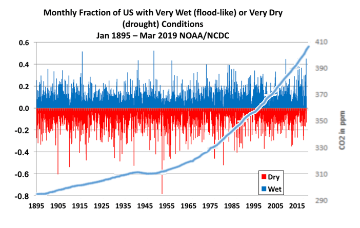
New research from The Australian National University (ANU) and ARC Centre of Excellence for Climate System Science suggests natural rainfall variation is so great that it could take a human lifetime for significant climate signals to appear in regional or global rainfall measures.

Even exceptional droughts like those over the Murray Darling Basin (2000-2009) and the 2011 to 2017 Californian drought fit within the natural variations in the long-term precipitation records, according to the statistical method used by the researchers.

This has significant implications for policymakers in the water resources, irrigation and agricultural industries.

“Our findings suggest that for most parts of the world, we won’t be able to recognise long term or permanent changes in annual rainfall driven by climate change until they have already occurred and persisted for some time,” said Professor Michael Roderick from the ANU Research School of Earth Sciences.

“This means those who make decisions around the construction of desalination plants or introduce new policies to conserve water resources will effectively be making these decisions blind.

“Conversely, if they wait and don’t act until the precipitation changes are recognised they will be acting too late. It puts policymakers in an invidious position.”

To get their results the researchers first tested the statistical approach on the 244-year-long observational record of precipitation at the Radcliffe Observatory in Oxford, UK. They compared rainfall changes over 30-year-intervals. They found any changes over each interval were indistinguishable from random or natural variation.

They then applied the same process to California, which has a record going back to 1895, and the Murray Darling Basin from 1901-2007. In both cases the long dry periods seem to fit within expected variations.

Finally, they applied the process to reliable global records that extended from 1940-2009. Only 14 per cent of the global landmass showed, with 90 per cent confidence, increases or decreases in precipitation outside natural variation.

Professor Graham Farquhar AO also from the ANU Research School of Biology said natural variation was so large in most regions that even if climate change was affecting rainfall, it was effectively hidden in the noise.

“We know that humans have already had a measurable influence on streamflows and groundwater levels through extraction and making significant changes to the landscape,” Professor Farquhar said.

“But the natural variability of precipitation found in this paper presents policymakers with a large known unknown that has to be factored into their estimates to effectively assess our long-term water resource needs.”  The research has been published in the journal Proceedings of the National Academy of Sciences.

us-wet-dry-co2rev-1

Summary

Much like sea level rise, scientists fearing the worst seek and hope to find a nanosignal inside noisy imprecise measurements of a naturally varying phenomenon.

Magnetic Pole Swapping and Cooling

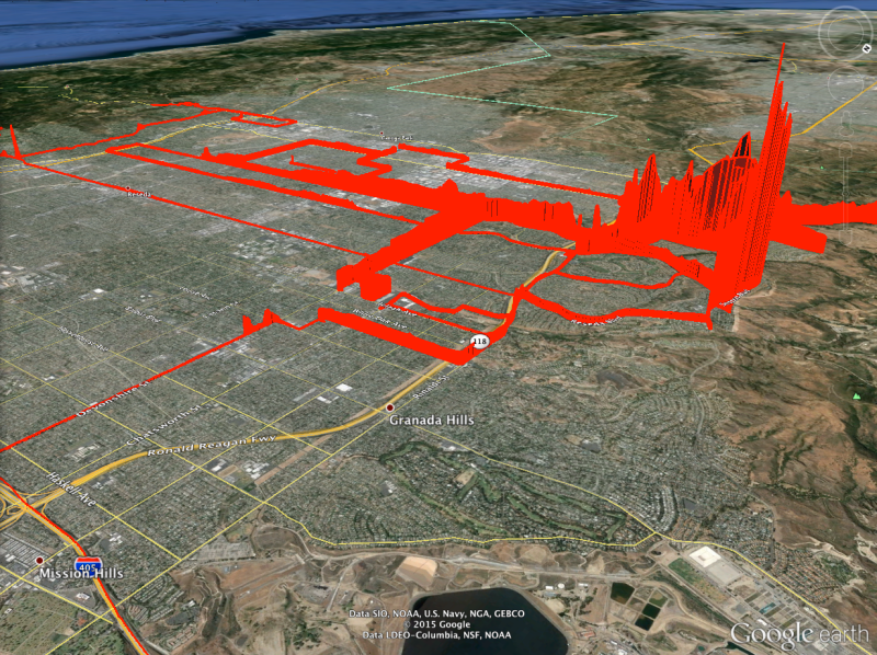
The Earth’s North magnetic pole has been wandering at 10-year intervals from 1970 to 2020, as seen in this animation from the National Centers for Environmental Information.

This post discusses solar and geologic magnetic pole swapping (not with each other of course) and the implications for humans. First the earth and later on the sun.

What On Earth?

Newsweek chose to report yesterday on earth’s meandering north pole as shown in the cool graphic above. That article (here) aims at sensational possible calamities, including high energy radiation, space particles, ozone depletion and electrical blackouts. A more sober assessment is provided by the conversation Why the Earth’s magnetic poles could be about to swap places – and how it would affect us By Phil Livermore and Jon Mound of U. Leeds.Excerpts below with my bolds.

The Earth’s magnetic field surrounds our planet like an invisible force field – protecting life from harmful solar radiation by deflecting charged particles away. Far from being constant, this field is continuously changing. Indeed, our planet’s history includes at least several hundred global magnetic reversals, where north and south magnetic poles swap places. So when’s the next one happening and how will it affect life on Earth?

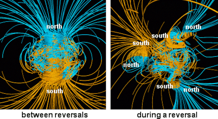
During a reversal the magnetic field won’t be zero, but will assume a weaker and more complex form. It may fall to 10% of the present-day strength and have magnetic poles at the equator or even the simultaneous existence of multiple “north” and “south” magnetic poles.

Geomagnetic reversals occur a few times every million years on average. However, the interval between reversals is very irregular and can range up to tens of millions of years.

There can also be temporary and incomplete reversals, known as events and excursions, in which the magnetic poles move away from the geographic poles – perhaps even crossing the equator – before returning back to their original locations. The last full reversal, the Brunhes-Matuyama, occurred around 780,000 years ago. A temporary reversal, the Laschamp event, occurred around 41,000 years ago. It lasted less than 1,000 years with the actual change of polarity lasting around 250 years.


In 2003, the so-called Halloween storm caused local electricity-grid blackouts in Sweden, required the rerouting of flights to avoid communication blackout and radiation risk, and disrupted satellites and communication systems. But this storm was minor in comparison with other storms of the recent past, such as the 1859 Carrington event, which caused aurorae as far south as the Caribbean.

The simple fact that we are “overdue” for a full reversal and the fact that the Earth’s field is currently decreasing at a rate of 5% per century, has led to suggestions that the field may reverse within the next 2,000 years. But pinning down an exact date – at least for now – will be difficult.

Since 2014, Swarm—a trio of satellites from the European Space Agency—has allowed researchers to study changes building at the Earth’s core, where the magnetic field is generated.

Historically, Earth’s North and South magnetic poles have flipped every 200,000 or 300,000 years—except right now, they haven’t flipped successfully for about 780,000 years. But the planet’s magnetic field is at long last showing signs of shifting.

The Earth’s magnetic field is generated within the liquid core of our planet, by the slow churning of molten iron. Like the atmosphere and oceans, the way in which it moves is governed by the laws of physics. We should therefore be able to predict the “weather of the core” by tracking this movement, just like we can predict real weather by looking at the atmosphere and ocean. A reversal can then be likened to a particular type of storm in the core, where the dynamics – and magnetic field – go haywire (at least for a short while), before settling down again.

The difficulties of predicting the weather beyond a few days are widely known, despite us living within and directly observing the atmosphere. Yet predicting the Earth’s core is a far more difficult prospect, principally because it is buried beneath 3,000km of rock such that our observations are scant and indirect. However, we are not completely blind: we know the major composition of the material inside the core and that it is liquid. A global network of ground-based observatories and orbiting satellites also measure how the magnetic field is changing, which gives us insight into how the liquid core is moving.

Solar Pole Swapping Puts Earth to Shame

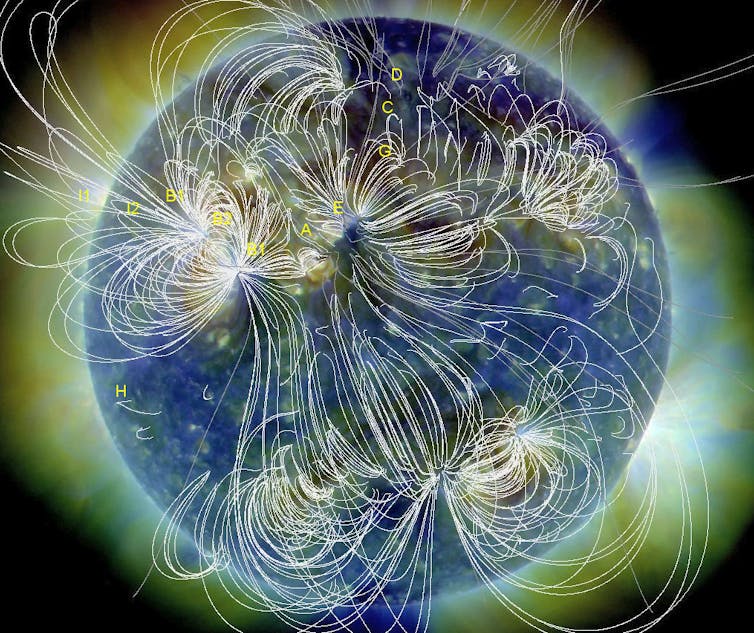
White lines show the magnetic field emanating from the sun’s surface. NASA

Background:

The sun as a whole also has a “global” magnetic field, oriented more or less north-south. So we can think of the sun as a large N-S magnet, like our Earth, but with smaller variously (but not randomly) oriented and continually evolving mini-magnets distributed over its photosphere (visible surface) and throughout its corona (extended atmosphere).

However, unlike our Earth, the sun’s large scale magnetic field flips over on a regular basis, roughly every 11 years. (Actually, Earth’s flips too, very irregularly. The last time was 780,000 years ago. But that’s another story.) Solar magnetic reversals occur close to solar maximum, when the number of sunspots is near its peak, though it is often a gradual process, taking up to 18 months.

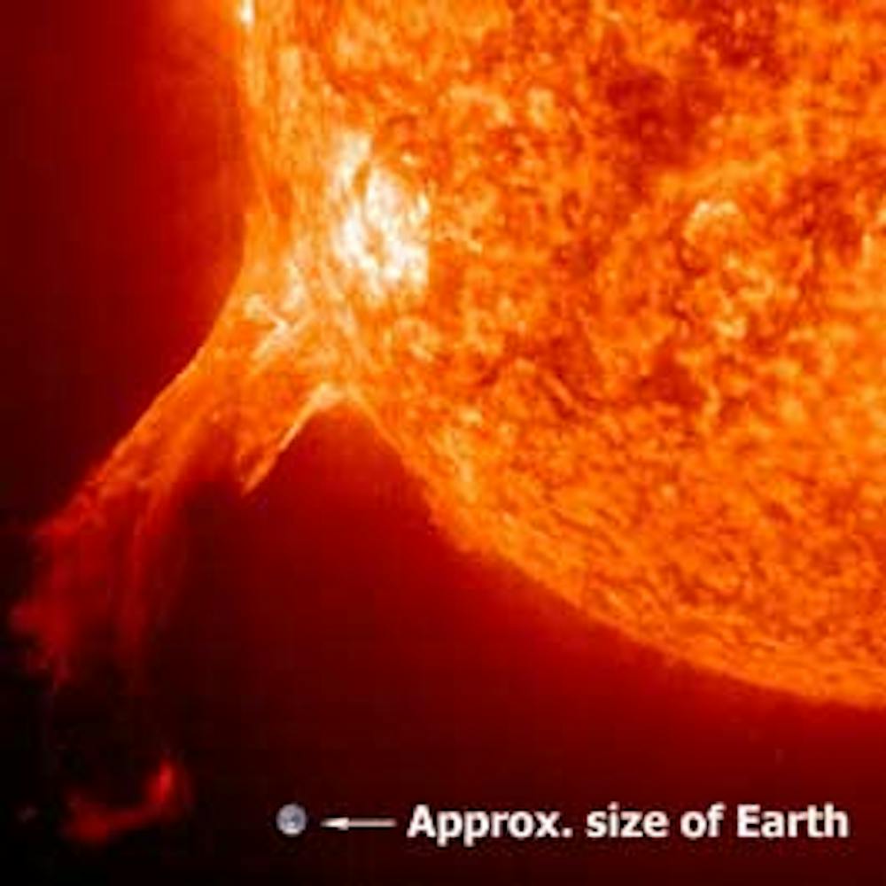
A solar flare (the white patch on the sun), and an erupting prominence reaching into space, are features of our active sun, and place the size of Earth in context. NASA

Paul Cally solar physicist Monash U (here)

About the Current Quiet Sun

Euan Mearns considers the implications at Energy Matters The Death of Sunspot Cycle 24, Huge Snow and Record Cold  Excerpts below with my bolds.

8 meter snow depth in Chamonix in the shadow of Mont Blanc in the French Alps January 2018

It looks like the snow in this drift is ~ 8m deep. And this is in the valley, not in the high basins where the snow fields that feed the glaciers lie. Now it’s obviously far too early to begin to draw any conclusions. But IF we get a run of 3 or 4 winters that dump this much snow, it is not inconceivable for me to imagine Alpine glaciers once again beginning to advance. I’m totally unsure how long it takes for pressure in the glacier source to feed through to advance of the snout.

So what is going on? We’ve been told by climate scientists that snow would become a thing of the past. We’ve also been told that global warming might lead to more snow and less snow. And we’ve been told that warming might even lead to cooling. The competing theory to the CO2 greenhouse is that the Sun has a prominent role in modulating Earth’s climate that was so eloquently described by Phil Chapman in his post earlier this week. This theory simply observes a strong connection between a weak solar wind (that is expressed by low sunspot numbers) and cold, snowy winters in the N hemisphere. Uniquely, most of those who argue for a strong solar influence also acknowledge the overprint of anthropogenic CO2. The IPCC effectively sets the Sun to zero. The Sun is entering a grand solar minimum already christened the Eddy Minimum by the solar physics community.

Figure 2 It is crucial to look at the baseline closely that in 2009 actually touched zero for months on end. This is not normal for the low point of the cycle. Figure 3 shows how cycle 24 was feeble compared with recent cycles. And it looks like it will have a duration of ~10 years (2009-2019) which as the low end of the normal range which is 9 to 14 years with mean of 11 years. Chart adapted from SIDC is dated 1 January 2018.

Mearns provides this summary of his article Cosmic Rays, Magnetic Fields and Climate Change

Cosmic rays are deflected by BOTH the Sun’s and Earth’s magnetic fields and there may also be variations in the incident cosmic ray background. Cosmogenic isotope variations, therefore, do not only record variations in solar activity.

This has two significant implications for me: 1) when I have looked into cosmogenic isotopes in the past I have been perplexed by the fact that in parts you see a wonderful coherence with “climate” (T≠climate) while else where, the relationship breaks down, and 2) my recent focus has been on variations in spectrum from the Sun (which may still be important) but to the extent that the Laschamp event (Earth’s magnetic field) may also be implicated in climate change then the emphasis needs to shift to cosmic rays themselves i.e. what Svensmark has been saying for years.

For readers not familiar with Earth’s magnetic field. It periodically flips but on a time-scale of millions of years. The N pole moves to the S pole and in the process of doing so the magnetic field strength collapses as evidenced by “Figure 7” in Phil’s post. The last time this happened was during the Laschamp event ~ 41,000 years ago. There was a full but short lived reversal, but the Earth’s magnetic field did collapse.

Now here’s the main point. We know that the glacial cycles beat to a 41,000 year rhythm that is the obliquity (tilt) of Earth’s axis. The magnetic field originates in Earth’s liquid mainly iron core. This raises the question, can changes in obliquity affect the geo-dynamo. You have to read what Phil has written closely:

Since we absolutely know (don’t we?) that the interglacial to glacial transitions of the current ice age are caused by Milankovitch forcing, the usual interpretation is that there must be some unknown mechanism by which changes in the orbit of the Earth and/or the tilt of the polar axis affect the geodynamo, triggering the excursions.

For decades to centuries, Earth’s N magnetic pole was pretty well fixed to a point in northern Canada. Not much in the news, but it has recently begun to migrate, quite rapidly.

For a more complete description of solar effects effects on earth’s climate see
The cosmoclimatology theory


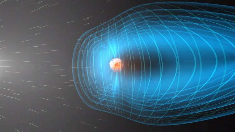
Earth’s magnetic field, in blue, shields the planet from the solar wind. NASA

Civil Climate Discourse

The issue of global warming/climate change has been used to polarize populations for political leverage. People like myself who are skeptical of alarmist claims find it difficult to engage with others whose minds are made up with or without a factual basis. In a recent email Alex Epstein gives some good advice how to talk about energy and climate. At the end I provide links to other material from Alex supporting his principle message regarding human benefits from using fossil fuels. Text below is his email with my bolds.

Two simple-but-powerful tactics

1. Opinion Stories

Unless I have some specific reason for wanting to have a long conversation I like to keep my conversations short, with the end goal of getting the other person to consume some high-impact resource.

One way to make this even more effective is to offer to email/mail the person a resource. Then you’ll have their contact info and can follow up in a few weeks.

The last paragraph of your message is really important. You’re telling the story of how you came to your opinion. I call this device “the opinion story.”

Here’s how it works.

Imagine you’re trying to persuade someone to read your favorite book. My favorite book is Atlas Shrugged, by Ayn Rand.

I used to say: “Atlas Shrugged is the best book you’ll ever read. You have to read it.”

That’s an opinion statement. If you haven’t read the book I’ll bet that statement makes you resistant. “Oh really? You’re telling me what the best book I’ll ever read is? You’re telling me what I have to read?”

Opinion statements often breed resistance and reflexive counter-arguments. So now I try to persuade people differently.

I might say: “My favorite book is Atlas Shrugged by Ayn Rand. I read it when I was 18 and the way the characters thought and approached life motivated me to pursue a career I love and give it everything I have.”

How do you react to that statement?

Probably better. You’re probably not resistant. You may well be intrigued. And you can’t disagree with me–because I didn’t tell you what to think, I told you my opinion story. I respected your independence.

While statements breed resistance and counter-argument, stories often breed interest and requests for more.

You can use opinion stories for anything, no matter how controversial.

For example, if someone asks me about my book, The Moral Case for Fossil Fuels, I don’t need to say “I prove that we should be using more fossil fuels, not less.” I can just say “I researched the pros and cons of different forms of energy and was surprised to come to the conclusion that we should be using more fossil fuels, not less.”

I like to have an opinion story for every controversial opinion I hold.

2. Introducing Surprising Facts

Reader Comment: “The problem I always run into is that they really believe Germany is a success.”

I’ve had the same experience, too! On many issues.

Often in conversation the phenomenon of conflicting factual claims on an issue—such as the impact of solar and wind on Germany’s economy—leads to an impasse.

One way to deal with this is to focus on establishing an explicit framework, with human flourishing (not minimum impact) as the goal and full context analysis (not bias and sloppiness) as the process. Most disputes stem from conflicting frameworks, not conflicting facts. And if you offer a compelling framework you’ll be more trustworthy on the facts.

That said, here’s a tactic I discovered a few years ago to make certain factual points much more persuasive in the moment..

I’ll start with how I discovered it.

I was walking through the Irvine Spectrum mall with a good friend when we ran into two young women working to promote Greenpeace.

My friend found one of the women attractive and said he wanted to talk to her. I thought, given my experiences with (paid) Greenpeace activists, that this was unlikely to be an edifying experience, and encouraged him to instead record a conversation between me and one of the women. Unfortunately for posterity, I was unpersuasive and what follows was never recorded.

I decided to talk to the other Greenpeace woman. She quickly started “educating” me on how Germany was successfully running on solar and wind.

Me: “Really? I’m curious where you’re getting that because I research energy for a living–and Germany is actually building a lot of new coal plants right now.”

Greenpeace: “No, that can’t be true.”

Me: “Okay, how about this? I’ll email you a news article about Germany building new coal plants. If I do, will you reconsider your position?” [Note: This is an example of the technique I recommended above.]

Greenpeace: Hesitates.

Me: “Actually, wait, we have smartphones. I’m going to Google Germany and coal. Let’s see what comes up.”

Displaying on my iPhone is a recent news story whose headline is something very close to: “Germany to build 12 new coal plants, government announces.”

Me: “So what do you think?”

Greenpeace: “I don’t know,” followed by—very rare for a Greenpeace activist—having nothing to say.

Had this been a normal person I am confident the live confirmation of the surprising fact would have made a lasting impression.

I think this tactic works best for news stories about surprising facts. Vs. an opinion story about some issue of analysis, like what Germany’s GDP is.

Summary

Alex Epstein is among those who demonstrate from public information sources comparisons between societies who use carbon fuels extensively and those who do not. The contrast is remarkable: Societies with fossil fuels have citizens who are healthier, live longer, have higher standards of living, and enjoy cleaner air and drinking water, to boot. Not only do healthier, more mobile people create social wealth and prosperity, carbon-based energy is heavily taxed by every society that uses it. Those added government revenues go (at least some of it) into the social welfare of the citizenry. By almost any measure, carbon-based energy makes the difference between developed and underdeveloped populations.

A previous post Social Benefits of Carbon referenced facts and figures from Alex’s book which can be accessed here

Other Resources:
Two Page Overview of The Moral Case for Fossil Fuels — What it is and why it matters 
main points are:
How to think about our energy future
Fossil fuels & human flourishing: the benefits
Fossil fuels & human flourishing: environmental concerns

11 page Introduction to The Moral Case for Fossil Fuels

Maslow’s hierarchy of human needs updated.

How’s Your CCIQ?


H/T David Wojick and CFACT

Doctors for Disaster Preparedness are concerned to be ready for real disasters and not be distracted by irrational fears like global warming/climate change. They have provided a useful resource for people to test and deepen their knowledge of an issue distorted for many people by loads of misinformation and exaggerations.

From David Wojick:

A new lesson set called the Climate Change IQ (CCIQ) provides a good skeptical critique of ten top alarmist claims. The format is succinct and non-technical. Each alarmist claim is posed as a question, followed by a short skeptical answer, which is highlighted with a single telling graphic.

Then there is a link to a somewhat longer answer, which in turn includes links to a few online sources of more information. Each lesson is also available in a printable PDF version, suitable for classroom use. This compact format is potentially very useful.

CCIQ comes from a long-standing skeptical group called the Doctors for Disaster Preparedness (DDP). Despite the name, DDP gives attention to pointing out scares that are not disasters waiting to happen. Not surprisingly climate alarmism gets a lot of this attention.

The ten topic questions are wide ranging, including the following. Each speaks to a popular pro-alarmist news hook.

Is climate change the most urgent global health threat?

Are government-sponsored climate scientists the only credible sources of information relating to climate-change policy?

Is the increase in atmospheric CO2 making wildfires worse?

Why can’t all States emulate California’s proposed “clean” energy standards?

What would happen if atmospheric CO2 concentration dropped by half, say to less than 200 ppm?

Are human CO2 emissions acidifying the oceans and endangering shell-making animals?

Will Manhattan and Florida soon be under water if humans do not curtail use of “fossil fuels”?

Do 97% of climate scientists agree that catastrophic climate change will result if humans do not curtail use of “fossil fuels”? (This one includes the dynamite John Christy graph showing the rapidly growing divergence of climate model global temperature forecasts with real world observations.)

Is Arctic ice disappearing?

And the number 1 CCIQ question: Would lowering atmospheric CO2 prevent or mitigate hurricanes?

Check it out. Inquiring minds want to know.


Natural Climate Factors: Snow

Variations in Siberian snow cover October (day 304) 2004 to 2016. Eurasian snow charts from IMS.

Previously I posted an explanation by Dr. Judah Cohen regarding a correlation between autumn Siberian snow cover and the following winter conditions, not only in the Arctic but extending across the Northern Hemisphere. More recently, in looking into Climate Model Upgraded: INMCM5, I noticed some of the scientists were also involved in confirming the importance of snow cover for climate forecasting. Since the poles function as the primary vents for global cooling, what happens in the Arctic in no way stays in the Arctic. This post explores data suggesting changes in snow cover drive some climate changes.

The Snow Cover Climate Factor

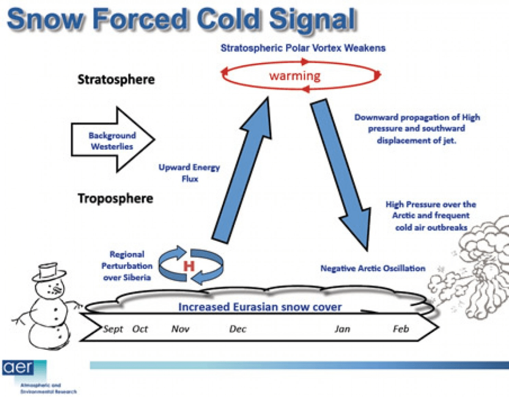
The diagram represents how Dr. judah Cohen pictures the Northern Hemisphere wintertime climate system.  He leads research regarding Arctic and NH weather patterns for AER.

cohen-schematic2

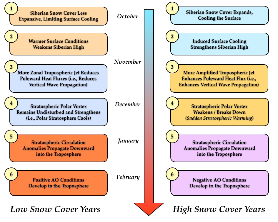
Dr. Cohen explains the mechanism in this diagram.

Conceptual model for how fall snow cover modifies winter circulation in both the stratosphere and the troposphere–The case for low snow cover on left; the case for extensive snow cover on right.

1. Snow cover increases rapidly in the fall across Siberia, when snow cover is above normal diabatic cooling helps to;
2. Strengthen the Siberian high and leads to below normal temperatures.
3. Snow forced diabatic cooling in proximity to high topography of Asia increases upward flux of energy in the troposphere, which is absorbed in the stratosphere.
4. Strong convergence of WAF (Wave Activity Flux) indicates higher geopotential heights.
5. A weakened polar vortex and warmer down from the stratosphere into the troposphere all the way to the surface.
6. Dynamic pathway culminates with strong negative phase of the Arctic Oscillation at the surface.

From Eurasian Snow Cover Variability and Links with Stratosphere-Troposphere
Coupling and Their Potential Use in Seasonal to Decadal Climate Predictions by Judah Cohen.

Observations of the Snow Climate Factor

The animation at the top shows from remote sensing that Eurasian snow cover fluctuates significantly from year to year, taking the end of October as a key indicator.

For several decades the IMS snow cover images have been digitized to produce a numerical database for NH snow cover, including area extents for Eurasia. The NOAA climate data record of Northern Hemisphere snow cover extent, Version 1, is archived and distributed by NCDC’s satellite Climate Data Record Program. The CDR is forward processed operationally every month, along with figures and tables made available at Rutgers University Global Snow Lab.

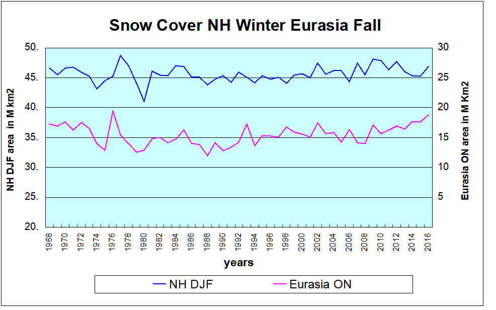
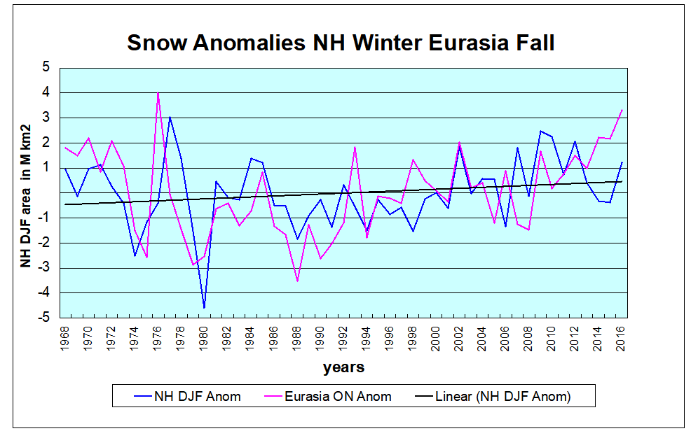
This first graph shows the snow extents of interest in Dr. Cohen’s paradigm. The Autumn snow area in Siberia is represented by the annual Eurasian averages of the months of October and November (ON). The following NH Winter is shown as the average snow area for December, January and February (DJF). Thus the year designates the December of that year plus the first two months of the next year.

Notes: NH snow cover minimum was 1981, trending upward since.  Siberian autumn snow cover was lowest in 1989, increasing since then.  Autumn Eurasian snow cover is about 1/3 of Winter NH snow area. Note also that fluctuations are sizable and correlated.

The second graph presents annual anomalies for the two series, each calculated as the deviation from the mean of its entire time series. Strikingly, the Eurasian Autumn flux is on the same scale as total NH flux, and closely aligned. While NH snow cover declined a few years prior to 2016, Eurasian snow is trending upward strongly.  If Dr. Cohen is correct, NH snowfall will follow. The linear trend is slightly positive, suggesting that fears of children never seeing snowfall have been exaggerated. The Eurasian trend line (not shown) is almost the same.

What About Winter 2017-2018?

These data confirm that Dr. Cohen and colleagues are onto something. Here are excerpts from his October 2 outlook for the upcoming season AER. (my bolds)

The main block/high pressure feature influencing Eurasian weather is currently centered over the Barents-Kara Seas and is predicted to first weaken and then strengthen over the next two weeks.

Blocking in the Barents-Kara Seas favors troughing/negative geopotential height anomalies and cool temperatures downstream over Eurasia but especially Central and East Asia. The forecast for the next two weeks across Central Asia is for continuation of overall below normal temperatures and new snowfall.

Currently the largest negative anomalies in sea ice extent are in the Chukchi and Beaufort Seas but that will change over the next month or so during the critical months of November-February. In my opinion low Arctic sea ice favors a more severe winter but not necessarily hemisphere-wide and depends on the regions of the strongest anomalies. Strong negative departures in the Barents-Kara Seas favors cold temperatures in Asia while strong negative departures near Greenland and/or the Beaufort Sea favor cold temperatures in eastern North America.

Siberian snow cover is advancing quickly relative to climatology and is on a pace similar to last year at this time. My, along with my colleagues and others, research has shown that extensive Siberian snow cover in the fall favors a trough across East Asia with a ridge to the west near the Urals. The atmospheric circulation pattern favors more active poleward heat flux, a weaker PV and cold temperatures across the NH. It is very early in the snow season but recent falls have been snowy across Siberia and therefore I do expect another upcoming snowy fall across Siberia.

Summary

In summary the three main predictors that I follow in the fall months most closely, the presence or absence of high latitude blocking, Arctic sea ice extent and Siberian snow cover extent all point towards a more severe winter across the continents of the NH.

Uh oh.  Now where did I put away my long johns?

Degrees of Climate Truth

Previous posts have dealt with science as a mode of inquiry, and described the process of theory and observation by which scientific knowledge is obtained. This post presents work by Andy May to classify the degrees of scientific certainty or truth, and apply these to climate claims.

The essay Facts and Theories comes from his blog Andy May Petrophysicist.
Excerpts below with my bolds.

Categories of Scientific Knowledge

Newton provided us with his descriptive “Law of Gravitation.” Newton’s law tells us what gravity does and it is very useful, but it tells us nothing about how it works. For that we need Einstein’s theory of relativity. Theories and laws are not necessarily related in science. A law simply describes what happens without describing why. A scientific theory attempts to explain why a relationship holds true.

In the scientific community, for both a law and a theory, a single conflicting experiment or observation invalidates them. Einstein once said:

“No amount of experimentation can ever prove me right; a single experiment can prove me wrong.”

So, let’s examine our topics in that light. Newton’s descriptive law of gravity, based on mass and distance, are there any exceptions? Not to my knowledge, except possibly on galactic sized scales, black holes and probably on very, very small sub-atomic scales. In everyday life, Newton’s law works fine. How about Einstein’s theory of gravity (Relativity), any exceptions? None that I know of at any scale.

How about evolution? Species evolve, we can see that in the geological record. We can also watch it happen in some quickly reproducing species. Thus we could describe evolution as a fact. It happens, but we cannot describe how without more work. Early theories of the evolutionary process include Darwin’s theory of natural selection and Lamarck’s theory of heritable species adaptation due to external stresses. Due to epigenetic research we now know that Darwin and Lamarck were both right and that evolution involves both processes. For a summary of recent research into the epigenetic component of evolution see this Oxford Journal article. Thus well-established facts and scientific laws rarely change but theories do evolve. I might add that while facts and laws don’t often change, they are easily dismissed when contradictory data are gathered. The modern theory of evolution is a good example of where competing theories can merge into one.

Most scientific theories begin as hypotheses. A hypothesis is best described as an idea of what might be causing a specific event to occur. A proper scientific hypothesis, like a theory, must be falsifiable. That is, we must be able to design an experiment or foresee an observation that will make the hypothesis false. “Climate change” is not falsifiable, it is not a scientific hypothesis or a theory. “Man-made climate change” is a scientific hypothesis since it is falsifiable. Hypotheses and theories are evolving things, new facts and observations cause them to change. In this way we build the body of science. Science is mostly skepticism. We look for what does not fit, we poke at established facts and laws, at theories and hypotheses. We try and find flaws, we check the numbers. Worse, science done properly means we spend more time proving ourselves wrong than we do proving we are right. Life is tough sometimes.

So how does this fit with the great climate change debate. I’ve made a table of phrases and identified each common phrase as a fact, theory, law, hypothesis, or simply an idea. These are my classifications and certainly open for debate.

In Table 1 we can see that the comparison of man-made climate change and the possibility of a man-made climate catastrophe are not really comparable to the theories of gravity and evolution. Man-made climate change is more than an idea, it is based on some observations and reasonable models of the process have been developed and can be tested. But, none of the models have successfully predicted any climatic events. Thus, they are still a work-in-progress and not admissible as evidence supporting a scientific theory.

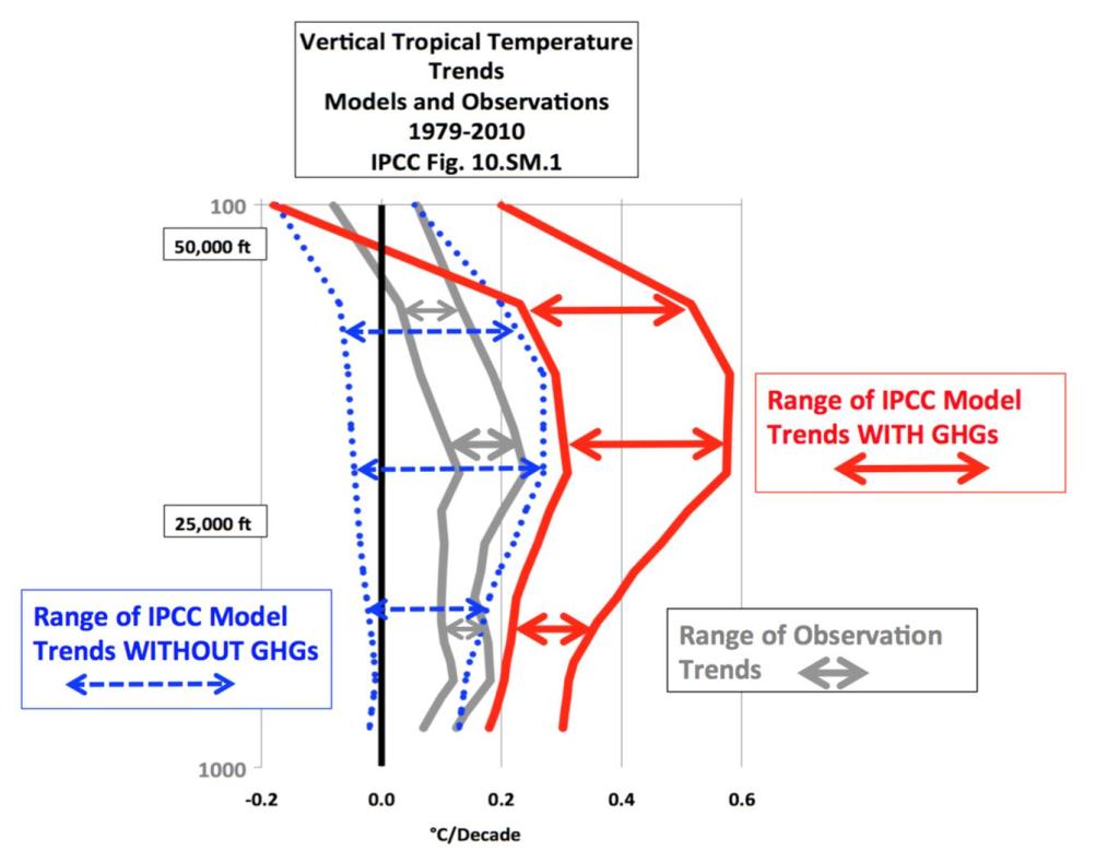
The idea of man-made climate change causing a catastrophe at the scale of Islamic terrorism is pure speculation. The models used to compute man’s influence don’t match any observations, this is easily seen in Figure 1 which is Dr. John Christy’s graph of the computer model’s predictions versus satellite and weather balloon observations. I should mention that satellite and weather balloon measurements are independent of one another and they are independent of the various surface temperature datasets, like HADCRUT and GHCN-M. All of the curves on the plot have been smoothed with five year averages.

The purple line going through the observations is the Russian model “INM-CM4.” It is the only model that comes close to reality. INM-CM4, over longer periods, does very well at hindcasting observed temperatures. This model uses a CO2 forcing response that is 37% lower than the other models, a much higher deep ocean heat capacity (climate system inertia) and it exactly matches lower tropospheric water content and is biased low above that. The other models are biased high. The model predicts future temperature increases at a rate of about 1K/century, not at all alarming and much lower than the predictions of the other models. (See Temperatures According to Climate Models)

One can consider each model to be a digital experiment. It is clear that the range of values from these digital experiments exceeds the predicted average temperature increase. This does not give us much confidence in the accuracy of the models. Yet, the IPCC uses the difference between the mean model temperature anomalies and observed surface temperatures since 1950 to compute man’s influence on climate.   (See Climate Models Explained)

In particular Soon, Connolly and Connolly (SCC15) believe that the IPCC chose an inappropriate model of the variation in the sun’s output (TSI or total solar irradiance). There are many models of solar variation in the peer reviewed literature and it is a topic of vigorous debate. Eight recent models are presented in Figure 8 of SCC15 (see Figure 3). Only low solar variability models (those on the right of Figure 3) are used by the IPCC to compute man’s influence on climate although just as much evidence exists for the higher variability models on the left. The scales used in the graphs are all the same, but the top and bottom values vary. At minimum, the IPCC should have run two cases, one for high variability and one for low. SCC15 clearly shows that the model used makes a big difference.

Any computer Earth model must establish a track record before it is used in calculations. The Earth is simply too complex and natural climate cycles are poorly understood. If natural cycles cannot be predicted they cannot be subtracted from observations to give us man’s influence on climate. The debate is not whether man influences climate, the debate is over how much man contributes and whether or not the additional warming dangerous. This observer, familiar with the science, would say the jury is still out. Certainly, the case for an impending catastrophe has not been made as this requires two speculative jumps. First, we need to assume that man is the dominant driver of climate, second we need to assume this will lead to a catastrophe. One can predict a possible catastrophe if the most extreme climate models are correct, but the record shows they are not. Only INM-CM4 matches observations reasonably well and INM-CM4 does not predict anything remotely close to a catastrophe.

In the study of the process of evolution the problem is the same. Some believe that the dominant process is natural selection and epigenetic change is minor. Some believe the opposite. Everyone believes that both play a role. As in climate science, figuring out which process is dominant is tough.

Recent climate history (the “pause” in warming) suggests that we have plenty of time to get our arms around this problem before doing anything drastic like destroying the fossil fuel industry and sending billions of people into poverty due to a lack of affordable energy.

Summary:  Scientific vs. Social Proof

In the IPCC reports certainty is presented in terms of social proofs. For example, an assertion is rated as Very High Confidence, or 95% Certain, meaning almost all consulted experts held that opinion. A claim rated as Moderate Confidence is in fact 50% Certain, meaning it is regarded as equally unlikely. Statements regarded as Low Confidence are thought to be so improbable that one wonders why they are presented. In any case, these are not scientific assessments, but rather opinion polling of people thought to be knowledgeable.

In contrast, Andy May demonstrates how scientific proof is obtained: A law or theory stands as along as no exceptions have been found. Or the law or theory is modified to stipulate more clearly under what conditions it operates. His classification of climate facts, theories and ideas sits well with me and helps to clarify what is presently known and unknown in this field.

As shown above, a theory or hypothesis falls if exceptions are observed.  Are there exceptions to the hypothesis of man-made global warming?  Yes, indeed there are many.  One of the most important disproofs (it only takes one) is actually provided by the climate models.

Figure 5. Simplification of IPCC AR5 shown above in Fig. 4. The colored lines represent the range of results for the models and observations. The trends here represent trends at different levels of the tropical atmosphere from the surface up to 50,000 ft. The gray lines are the bounds for the range of observations, the blue for the range of IPCC model results without extra GHGs and the red for IPCC model results with extra GHGs.The key point displayed is the lack of overlap between the GHG model results (red) and the observations (gray). The nonGHG model runs (blue) overlap the observations almost completely.

IPCC Assessment Reports show that the IPCC climate models performed best versus observations when they did not include extra GHGs and this result can be demonstrated with a statistical model as well.

Full explanation at Warming from CO2 Unlikely

For more on measurements and science see Data, Facts and Information