Koonin’s Climate Honesty
Steven Koonin shared his honest and wise perspective on global warming/climate change in the interview above. For those who prefer reading, an excerpted transcript from the closed captions provides the highlights in italics with my bolds and added images.
PR: Welcome to uncommon knowledge; I’m Peter Robinson. Now a professor at New York University and a fellow at the Hoover Institution, Steven Koonin received a Bachelor of Science degree at Caltech and a doctorate in physics at MIT during a career in which he published more than 200 peer-reviewed scientific papers and a textbook on computational physics. Dr Koonin rose to become Provost of Caltech. In 2009 President Obama appointed him under Secretary of science at the Department of Energy a position Dr Koonin held for some two and a half years. During that time he found himself shocked by the misuse of climate science in politics and the press. In 2021 Dr Koonin published Unsettled. What climate science tells us, what it doesn’t and why it matters.
In Unsettled you write of a 2014 workshop for the American physical society, which means it’s you and a bunch of other people who I cannot even begin to follow. Serious professional scientists such as you and several colleagues were asked to subject current climate science to a stress test: to push it, to prod, to test it to see how good it was. From Unsettled I’m quoting you now Steve:
“ I’m a scientist; I work to understand the world through measurements and observations. I came away from the workshop not only not only surprised but shaken by the realization that climate science was far less mature than I had supposed.”
Let’s start with the end of that. What had you supposed?
SK: Well I had supposed that humans were warming the globe; carbon dioxide was accumulating in the atmosphere causing all kinds of trouble, melting ice caps, warming oceans and so on. And the data didn’t support a lot of that. And the projections of what would happen in the future relied on models that were, let’s say, shaky at best.
PR: All right. Former Senator John Kerry is now President Biden’s special Envoy for climate. Let me quote from John Kerry in a 2021 address to the UN Security Council:
“Net zero emissions by 2050 or earlier is the only way that science tells us we can limit this planet’s warming to 1.5 degrees Celsius. Why is that so crucial? Because overwhelming evidence tells us that anything more will have catastrophic implications. We are Marching forward in what is tantamount to a mutual suicide pact.”
Overwhelming evidence science tells us. What’s wrong with that?
SK: Well you should look at the actual science which I suspect that Ambassador Kerry has not done. The U.N puts out assessment reports every five or six years. Those are by the IPCC the Intergovernmental Panel for Climate Change and are meant to survey, assess and summarize the state of our knowledge about the climate. The most recent one came out about a year ago in 2022, the previous one in 2014 or so.
Those reports are massive to read; the latest one is three thousand pages and it took 300 scientists a couple years to write. And you really need to be a scientist to understand them. I have a background in theoretical physics, I can understand this stuff. But still it took me a couple years to really understand what goes on. Now Ambassador Kerry and other politicians certainly have not done that.
Likely he’s getting his information from the summary for policy makers, or more likely for an even further boiled down version. And as you boil down the good assessment into the summary, into more condensed versions, there’s plenty of room for mischief. That Mischief is evident when you compare what comes out the end of that game of telephone with what the actual science really is.
PR: All right: what we know and what we don’t. Let’s start with what we know. I’m quoting you again Steve from Unsettled “Not everything you’ve heard about climate science is wrong.” In particular you grant in this book two of the central premises or conclusions of climate science that the Press is always telling us about. here’s one and again I’m going to quote you:
“Surely we can all agree that the globe has gotten warmer
over the last several decades.”
SK: No debunking. In fact it’s gotten warmer over the last four centuries Now that’s a different assertion, but it’s equally supported by the assessment reports. We’ll have to come back to that because the time scale is important. It’s one thing to say this about in my own lifetime the the the climate of the the surface of this planet, and it’s an entirely different thing to say beginning 150 years before this nation was founded temperatures began to rise.
PR: Yes, it’s a different statement but it’s equally true and has some bearing on the warming that we’ve seen over the last century. Here’s the premise that you do grant again I’m going to quote Unsettled
“There is no question that our emission of greenhouse gases in particular CO2 is exerting a warming influence on the planet.” We’re pumping CO2 into the atmosphere, CO2 is a greenhouse gas it must be having some effect of course.”
Absolutely that’s as far as you’re willing to go. But then you say so actually those are pretty two benign premises that you grant: the Earth has been warming and it’s been warming for a long time. CO2 is a greenhouse gas and it must be having some effect it’s coming from human activities and it’scoming from Humanity, mostly fossil fuels. Now now on to what we don’t know okay again from Unsettled
“Even though human influences could have serious consequences for the climate, they are small in relation to the climate system as a whole. That sets a very high bar for projecting the consequences of human influences.”
That is so counter to the general understanding that informs the headlines, particularly this hot summer we’ve had . So explain that.
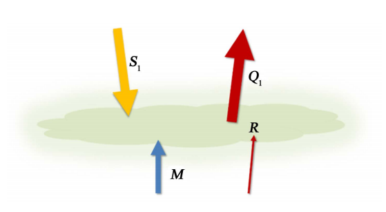
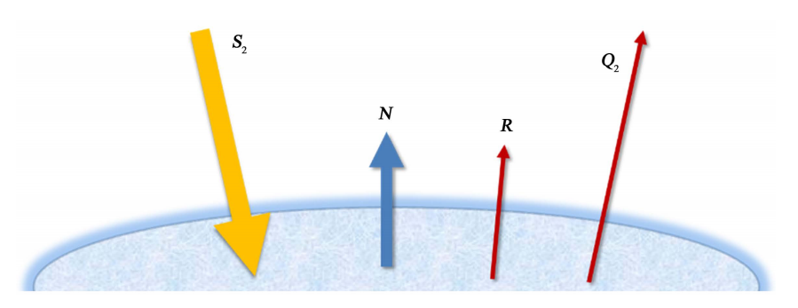
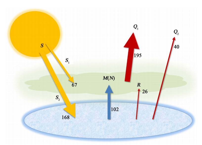
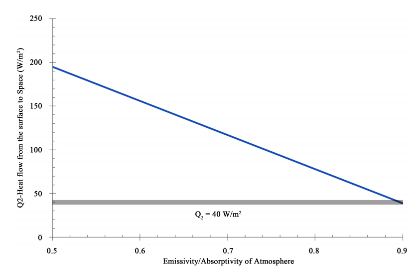
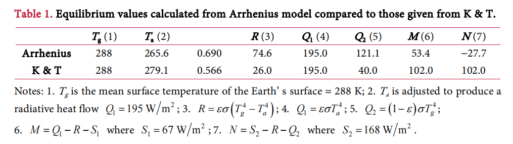
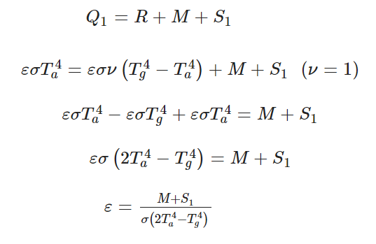
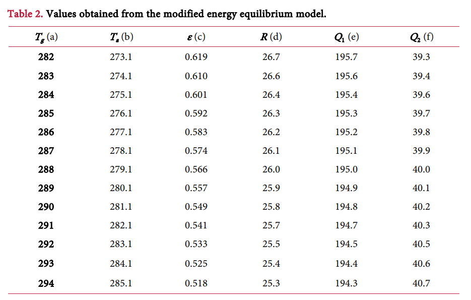
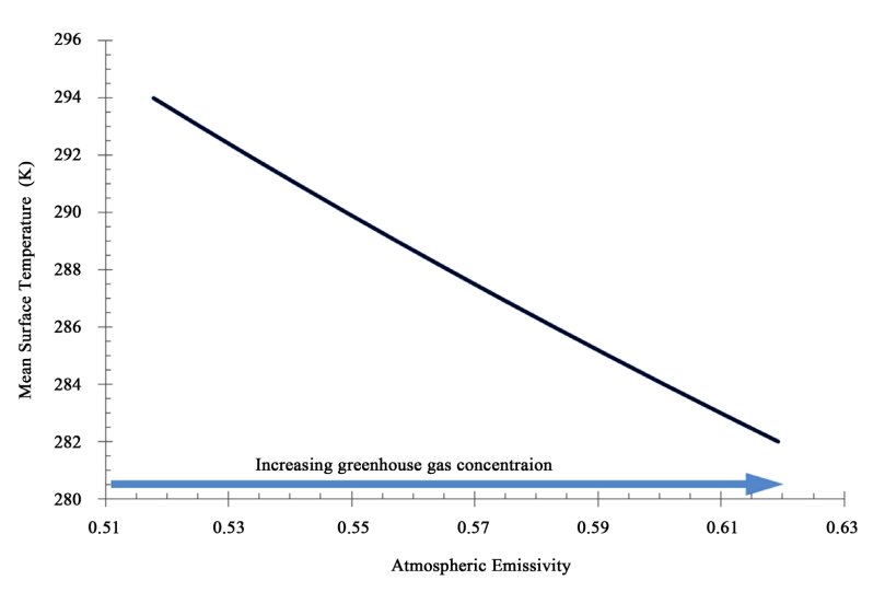
SK: Human influences as described in the IPCC are a one percent effect on the radiation flow–the flow of heat radiation and sunlight in the atmosphere. That means your understanding had better be at the one percent level or better if you’re going to predict how the climate system is going to respond. And the one percent makes sense because the changes in temperature we’re talking about are three degrees Kelvin right whereas the average temperature of the earth is about 300 degrees Kelvin.
PR: So human influences are a one percent effect on a complicated chaotic multi-scale system for which we have poor observations You seem to you seem to quite relaxed about the original science
SK: The underlying science is expressed in the data and expressed in the research literature the journals the research papers that people produce the conference proceedings and so on. The IPCC takes those and assesses and summarizes them and in general it does a pretty good job at that level. And there’s not going to be much politics in that although they might quibble among themselves about adjectives and adverbs; this is extremely certain or this is unlikely or highly unlikely and so on. But by and large it’s pretty good, this is done by fellow Professionals in a professional manner
Now things begin to go wrong. The next step is because nobody who isn’t deeply in the field is going to read all that stuff, so there is a formal process to create a summary for policy makers which is initially drafted by the governments not by the scientists. Well it’s not of course all of them, there’s some subcommittee to do the summary for policy makers and that gets drafted and passed by the scientists for comment. In the end it’s the governments who have approved the summary for policy makers line by line and that’s where the disconnect happens.
For the disconnect I’ll give you an example. Look at the most recent report and the summary for policy makers is talking about deaths from extreme heat incremental deaths and it says that you know extreme heat or heat waves have contributed to uh mortality okay and that’s a true statement But they forgot to tell you that the warming of the planet decreases the incidence of extreme cold events. And since nine times as many people around the globe die from extreme cold than from extreme heat, the warming from the planet has actually cut the number of deaths from extreme temperatures by a lot. That’s not in there at all.
So the statement was completely factual, but factually incomplete
in a way meant to alarm, not to inform.

And then John Kerry stands up and gives a speech. Maybe he read the SPM I don’t know or his staff read it and probably some of their talking points. And so you get Kerry saying that, you get the Secretary General of the U.N Gutierrez saying, we’re on a highway to climate hell with our foot on the accelerator. But they’re Preposterous of course, even by the IPCC reports they’re Preposterous. The climate scientists are negligent for not speaking up and saying that’s not okay.
PR: Another one of the things going wrong you write about in a way that I have never seen anyone write about computer models. I have never seen anybody make computer models interesting. So congratulations Steve you did something special as far as I know in the entire Corpus of English language.
Here I’m going to quote from a piece you published in the Wall Street Journal not long ago:
“Projections of future climate and weather events rely on models
demonstrably unfit for the purpose.”
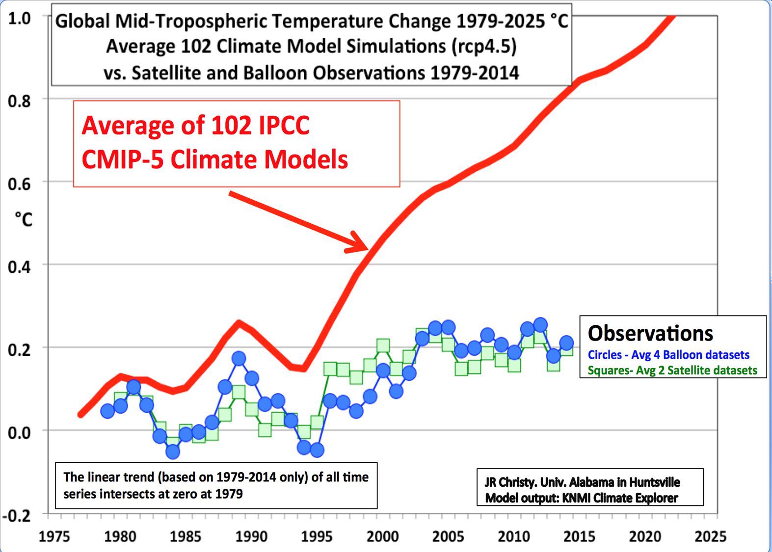
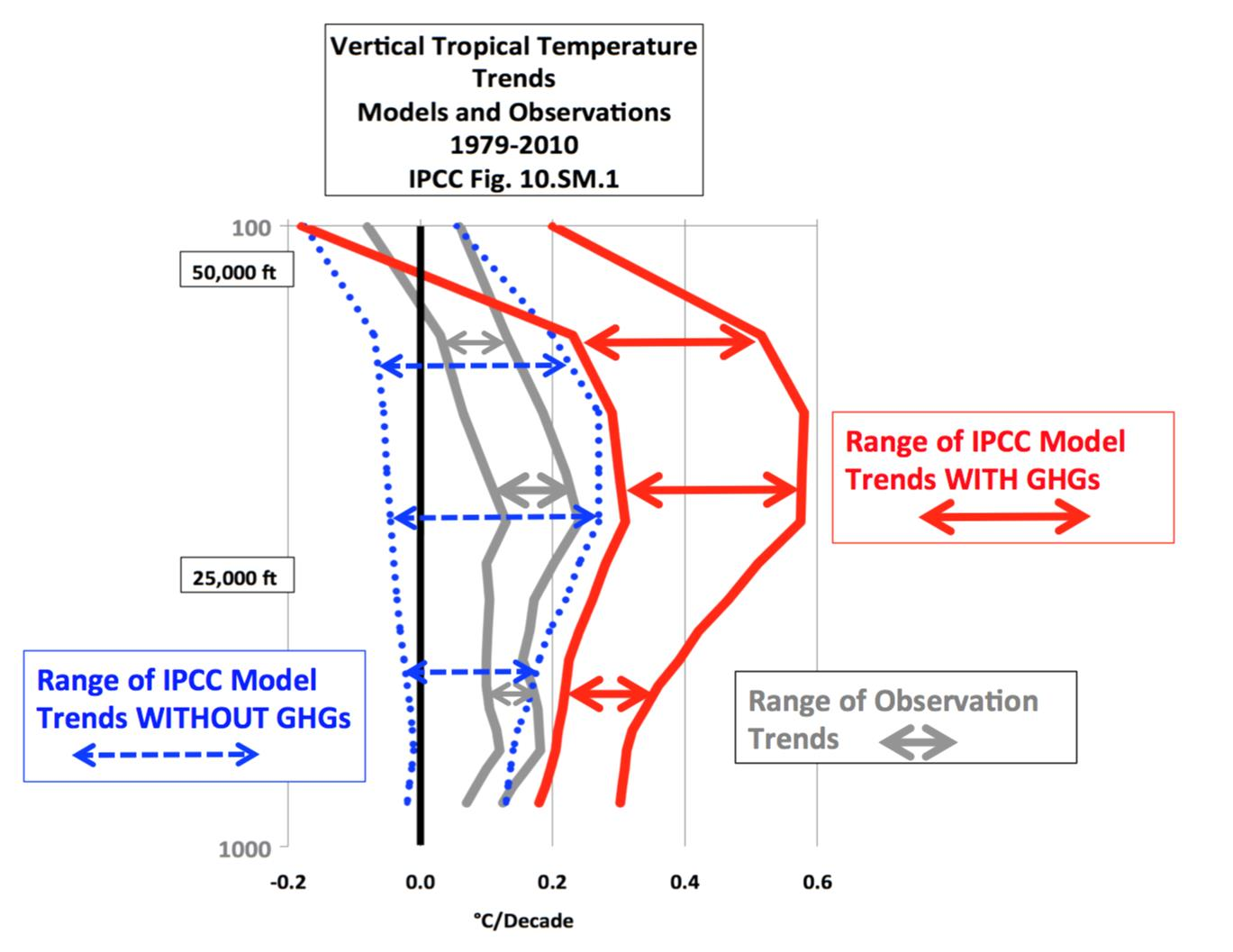
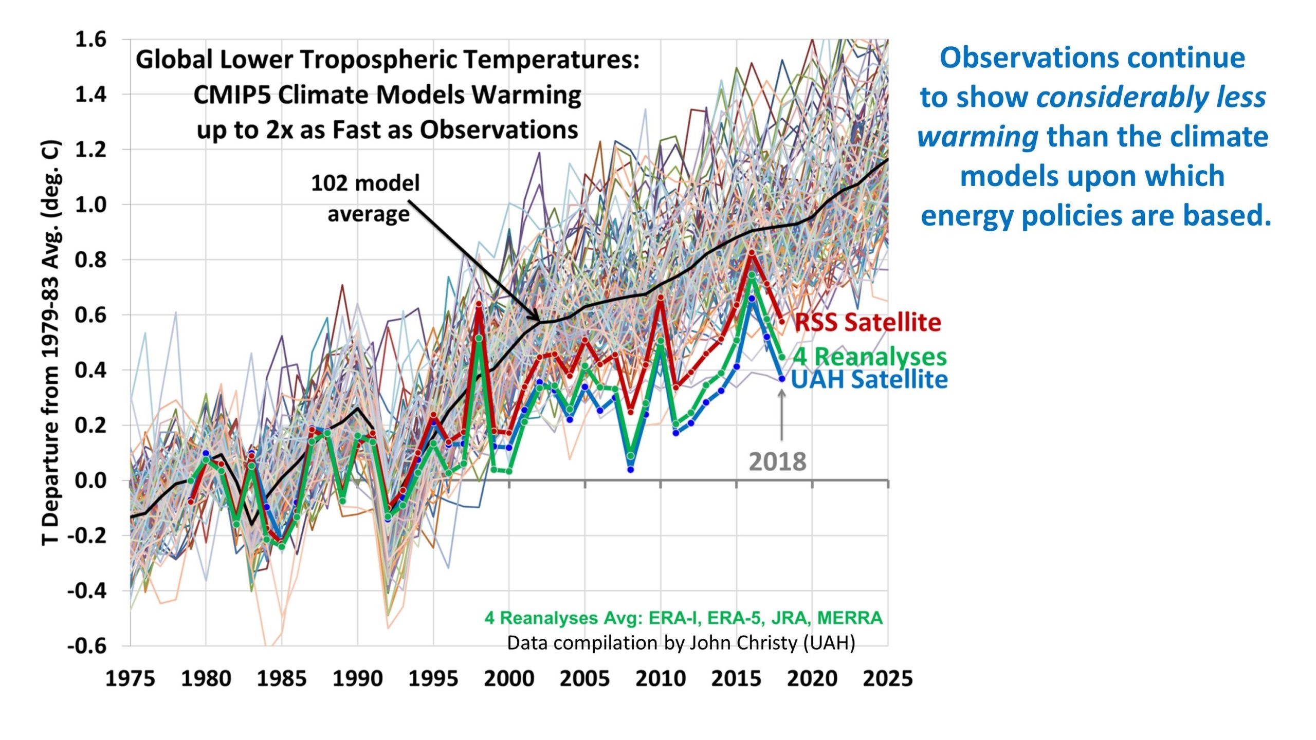
SK: Well, to make a projection of future climate you need to build this big complicated computer model which is really one of the grand computational challenges of all time.
This is not something I wrote a textbook in 1980s when the first PCS came out about how to do modeling on computers with physics. I do know what I’m talking about okay. And then you have to feed into the model what you think future emissions are going to be and the IPCC has five or six different scenarios, High emissions ,low emissions. If you take a particular scenario and feed it into the roughly 50 different models that exist that are developed by groups around the world
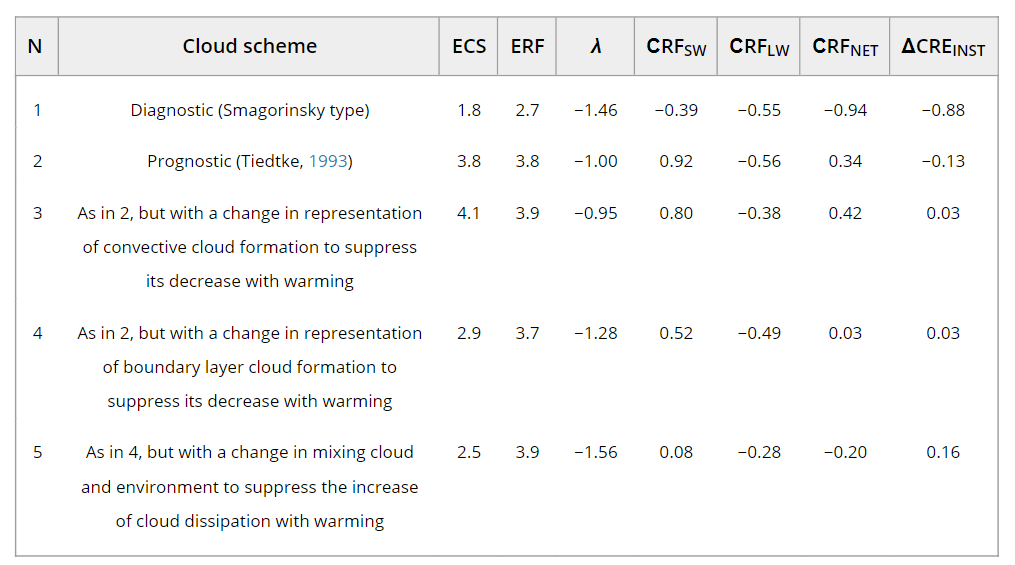
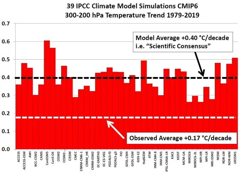
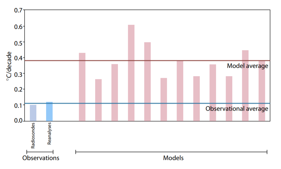
So Caltech has a model, Harvard has a model, yeah Oxford. But the Chinese have several models, the Russians and so on. When you feed the same scenario into those different models you get a range of answers. The range is as big as the change you’re trying to describe itself okay, And we can go into the reasons why there is that uncertainty, and in the latest generation of models about 40 percent of them were deemed to be too sensitive to be of much use.
.PNG)
Too sensitive meaning that when you add the carbon dioxide in and the temperature goes up too fast compared to what we’ve seen already. So that’s really disheartening the world’s best models are trying as hard as they can, and they get it very wrong at least 40 percent of the time.
This is not only my assessment you can look at papers published by Tim Palmer and Bjorn Stevens who are serious modelers in the consensus. And their own phrases are that these models are not fit for purpose. at least at the regional or more detailed Global level .
PR: Quoting Unsettled again, and this is one of the most astonishing passages in the book. Writing about the effects of the increases in computing power over the years:
“Having better tools and information to work with should make the models more accurate
and more in line with each other. This has not happened.
The spread in results among different computer models is increasing.”
This one you’re going to have to explain to me. As our modeling power, as our processing power increases, we should be closing in on reliable conclusions and yet they seem to be receding faster than we can approach them. if I got that correct that’s right how can that be
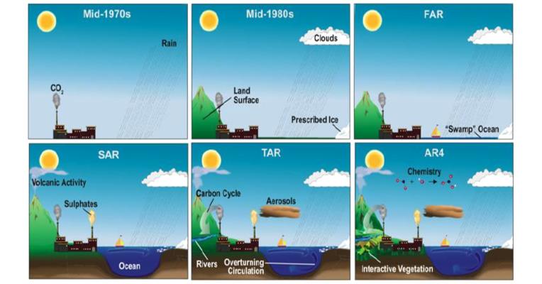
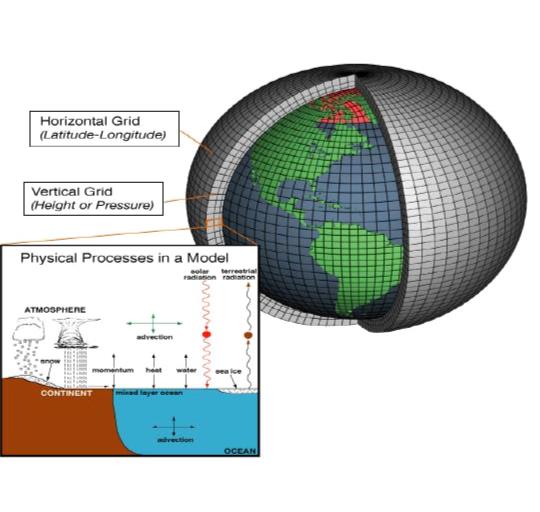
SK: Because as the models become more sophisticated that means either you made the boxes a little bit smaller in the model the grid boxes so there are more of them or you made more sophisticated your description.
The whole globe is sort of divided into 10 million slabs really. The average size of a grid box in the current generation is 100 kilometers 60 miles okay and within that 60 miles there’s a lot that goes on that we can’t describe explicitly in the computer because clouds are maybe five kilometers big and Rain happens here and not there within the grid box we can’t describe all that.
One day we’ll be able to , but not really very soon and let me explain why. The current grid boxes are 100 kilometers so you might say well why not make them 10. well suddenly the number of boxes has gone up by a hundred okay so you need a hundred times more powerful computer but it’s worse than that because the time steps have to be smaller also because things shouldn’t move more than a grid box in one time step and so the processing power actually goes up as the cube of the grid size and so if you want to go from 100 kilometers to 10 kilometers that’s a factor of 10. the processing power required goes up by a factor of a thousand and it’s going to be a long time before we got a computer that’s a thousand times more powerful than what we have.
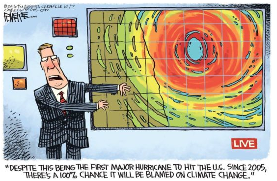
PR: You and I are speaking in the middle of August I just started collecting headlines thinking I’ll just read this to Steve and see what he says about it.
CBS News this past May “Scientists say climate change is making hurricanes worse.”
Koonin in Unsettled: “Hurricanes and tornadoes show no changes attributable to human influences.”
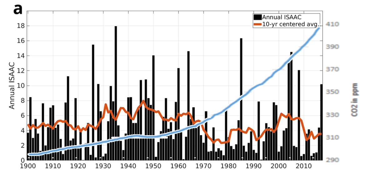
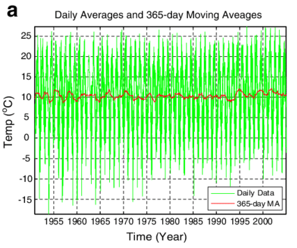
[The graph above shows exhibit 2a from Truchelut and Staehling overlaid with the record of atmospheric CO2 concentrations. From NOAA combining Mauna Loa with earlier datasets.]
To determine Integrated Storm Activity Annually over the Continental U.S. (ISAAC) from 1900 through 2017, we summed this landfall ACE spatially over the entire continental U.S. and temporally over each hour of each hurricane season. We used the same methodology to calculate integrated annual landfall ACE for five additional geographic subsets of the continental U.S.
SK: Well you know what science does CBS know? The media gets their information from reporters who have no or very little scientific training. (PR: you mean you didn’t graduate people from Caltech who went to work there?) Probably one or so and they do a good job. But they have reporters on a climate beat who have to produce stories the more dramatic the better: If it bleeds It leads. and so you get that kind of stuff I quote
When I say something about hurricanes, I quote right from the IPCC reports and it doesn’t say that at all. Actually the most recent report said it based on a paper which was subsequently corrected
PR: Floods here’s a 2020 headline this is from an article or press release published by the UN environment program quote climate change this is the U.N now not the IPCC but it is a U.N agency:
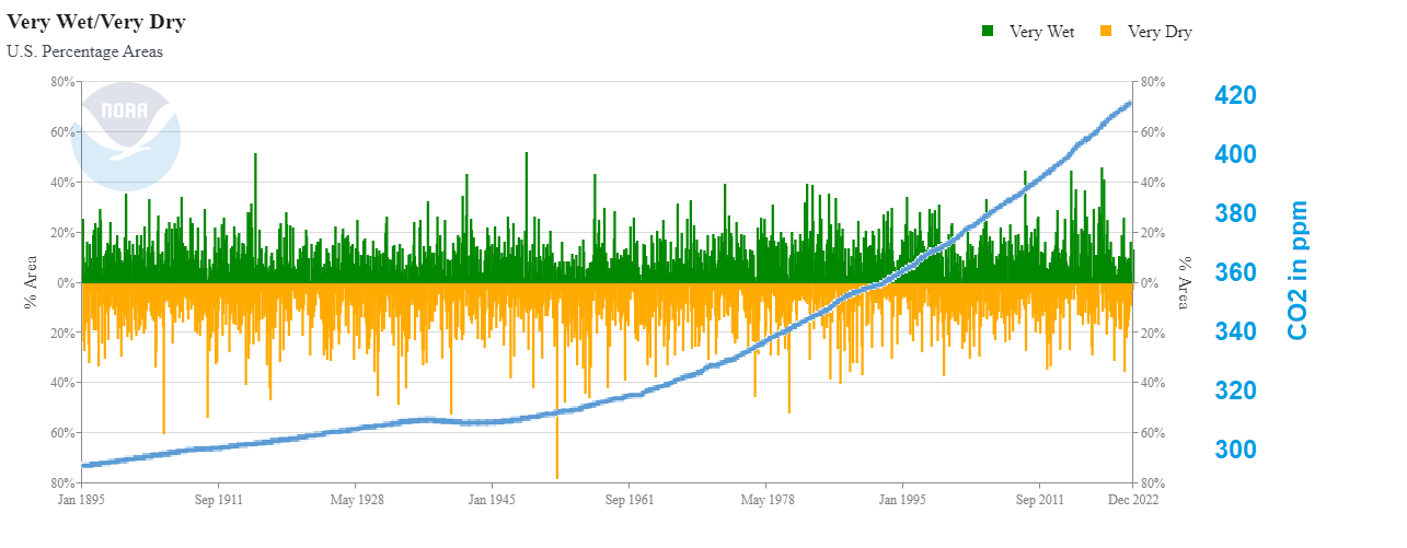
UNEP: “Climate change is making record-breaking floods.”
Steve Koonin in Unsettled: “We don’t know whether floods globally are increasing, decreasing or doing nothing at all.”
SK: I would say the U.N needs to be consistent and and they should check their press release against the IPCC reports before they say anything.
When I wrote unsettled I tried very hard to stick with the gold standard which was the IPCC report at the time or the subsequent research literature I had available to me when I wrote the book only the fifth assessment report which came out in 2014 as we’ve discussed.
The sixth assessment report came out about a year ago and I’m proud to say there’s essentially nothing in there now that needs to be changed in the paperback edition. I will do an update of course but the paperback edition is not going to be totally rewritten.
PR: All right agriculture. Here’s a 2019 headline
New York Times: “Climate change threatens world’s food supply United Nations warns.”
Steve Koonin in Unsettled: “Agricultural yields have surged during the past Century even as the globe has warmed. And projected price impacts from future human induced climate changes through 2050 should hardly be noticeable among ordinary market dynamics.”

SK: It’s not what I said but what the IPCC said. Take current media and almost any climate story, I can write a very effective counter-– it’s like shooting fish in a barrel. I’ve got I’ve actually gotten to the point where I say oh no not another one do I have to do that too. So this is endemic to a media that is ill-informed and has an agenda to set.
The agenda is to promote alarm and induce governments to decarbonize.
I think that probably the primary agenda is to get clicks and eyeballs but and you know there are organizations it’s wonderful there’s an organization called Covering Climate Now which is a non-profit membership organization it’s got the guardian it’s got various other media NPR I believe and their mission is to promote the narrative. They will not allow anything to be broadcast or written that is counter to the narrative The Narrative is: We’ve already broken the climate.
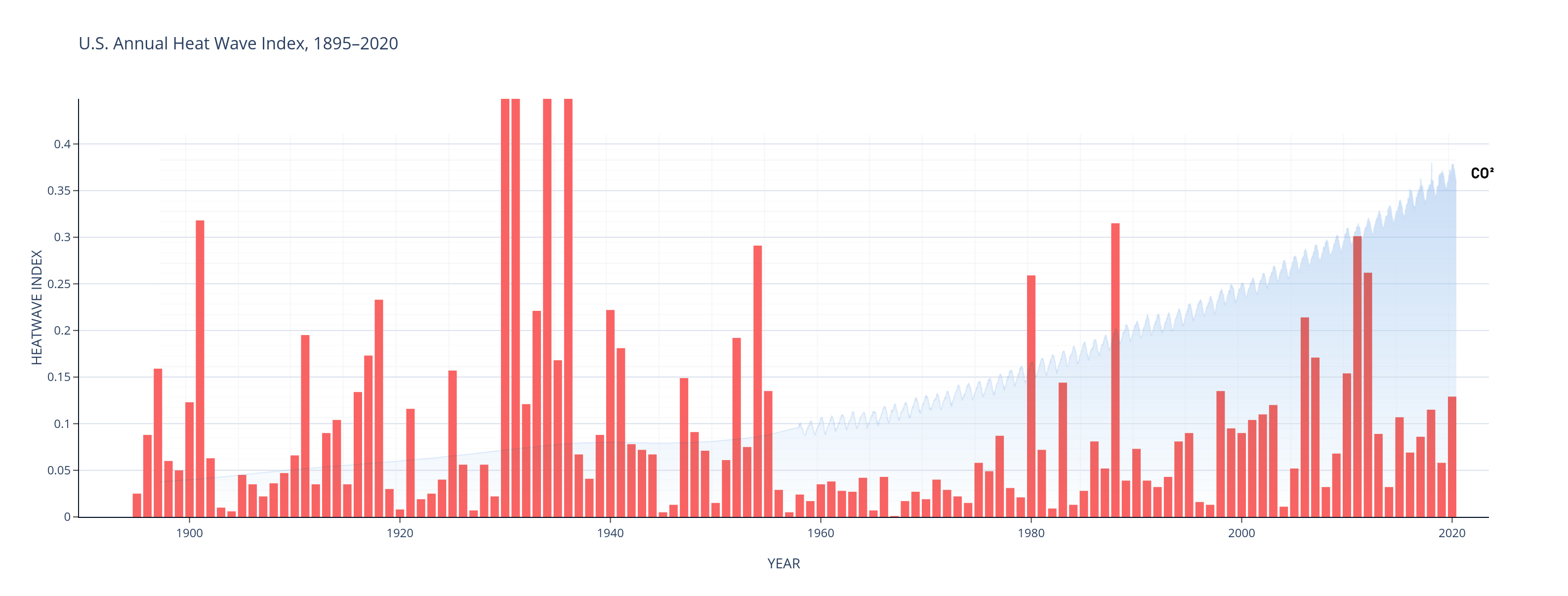
PR: These are headlines in July of 2023. This is last month here as you and I tape this.
New York Times on July 6th: ” Heat records are broken around the globe as Earth warms fast from north to south. Temperatures are surging as greenhouse gases combined with the effects of El Nino.“
New York Times on July 18: “Heat waves grip three continents as climate change warms Earth. Across North America, Europe and Asia hundreds of millions endured blistering conditions. A U.S official called it a threat to all humankind.”
Wall Street Journal on July 25th: “July heat waves nearly impossible without climate change study says. Record temperatures have been fueled by decades of fossil fuel emissions.”
New York Times on July 27th; “This looks like Earth’s warmest month, hotter ones appear to be in store. July is on track to break all records for any month scientists say, as the planet enters an extended period of exceptional warmth.”
Unsettled came out in April 2021 so we will forgive you not knowing in April 2021 what would happen last month July of 2023. But now July 2023 is in the record books, and doesn’t it prove that climate science is settled?
SK: That statement together with all those headlines confuse weather and climate. So weather is what happens every day or maybe even every season; climate the official definition is a multi-decade average of weather properties. That’s what the IPCC and another U.N agency, the World Meteorological organization (WMO) says.
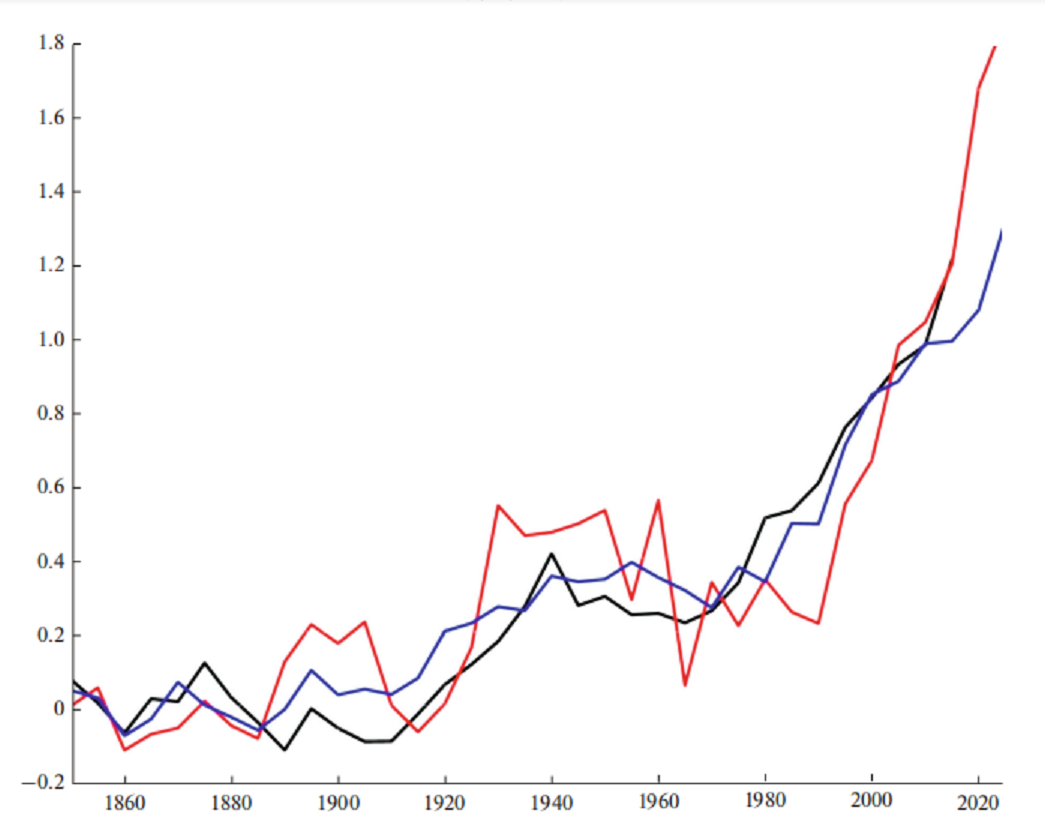
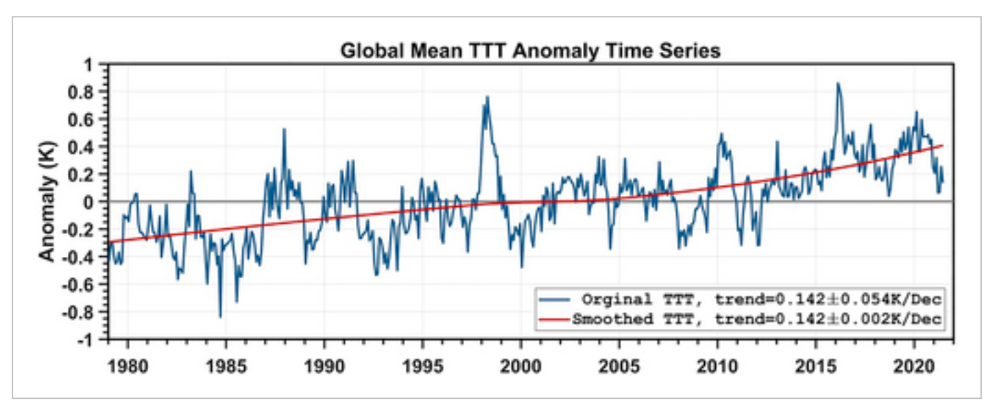
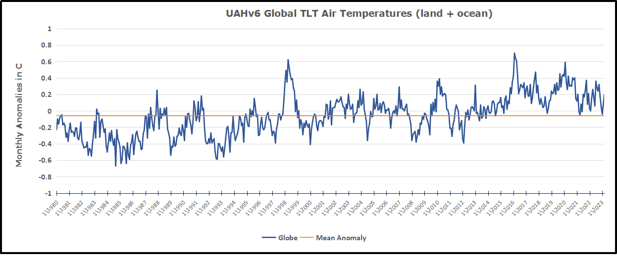
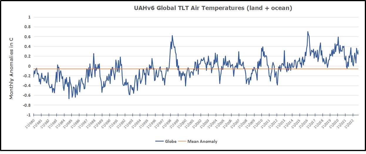
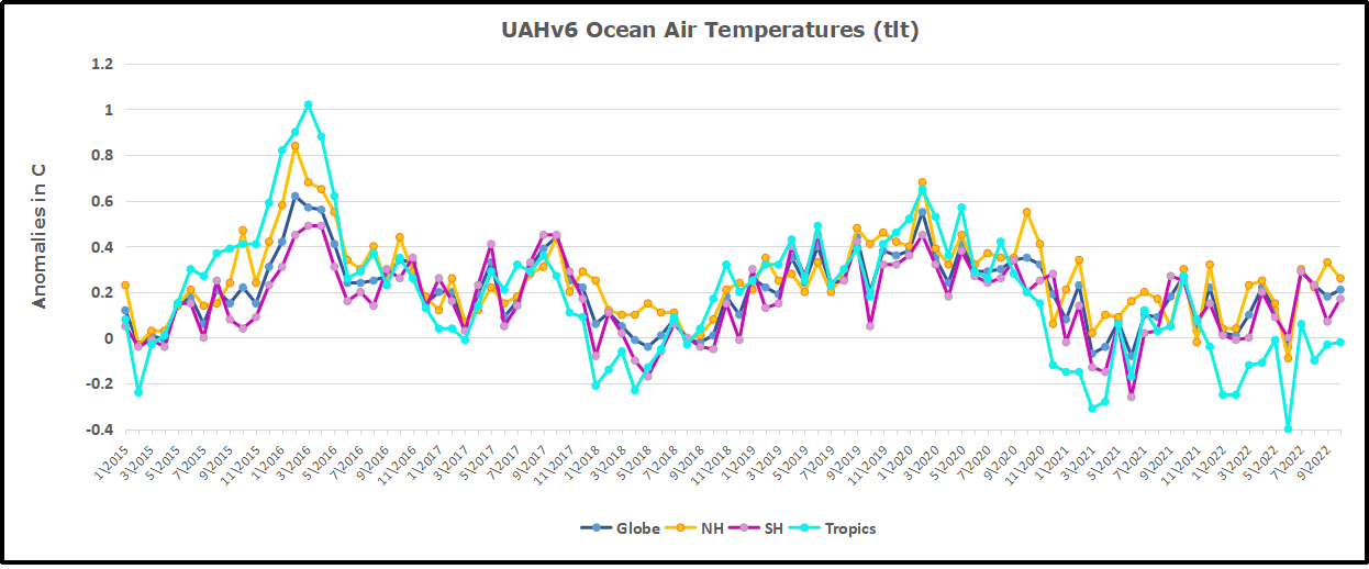
We have satellites that are continually monitoring the temperature of the atmosphere and they report out every month what the monthly temperature is or more precisely what the monthly temperature anomaly is namely how much warmer or colder is it than the average what would have been expected for that month. We have data that go back to about 1979. so we have good monthly measures of the global temperature on the lower atmosphere for 40 something years.
You see month-to-month variations of course but a long-term Trend that’s going up no question about it. I I won’t get the number exactly right, but it’s going up at about 0.13 degrees per decade all right. That’s some combination of natural variability and greenhouse gases. Human influences are more general and then every couple years you see a sharp Spike going up, and that’s El Nino. It’s weather, and so it goes up and then goes back down.
So there’s a long-term Trend which is greenhouse gases and natural variability and then there’s this natural Spike every once in a while, but an eruption goes off you see something, El Ninos happen you see something. And so on the last month in July there was another Spike in the anomaly the anomalies about as large as we’ve ever seen but not unprecedented okay
The real question is why did it Spike so much right?
Nothing to do with CO2
CO2 is kind of the well human influences a kind of the base on which this uh phenomenon occurs so because the the CO2 even if you stipulate that CO2 is causing some large proportion of this warming, it’s a slow steady process you would not expect to see spikes you wouldn’t expect to see sudden step functions absolutely not all right and there are various reasons people hypothesize we don’t know yet why we’ve seen the spike in the last month
PR: You better take just a moment to explain what is El Nino
SK: El Nino is a phenomenon in the climate system that happens once every four or five years heat builds up in the equatorial Pacific to the west of Indonesia and so on and then when enough of it builds up it kind of surges across the Pacific and changes the currents and the winds uh as it surges toward South America all right it was discovered in the 19th century and it kind of well understood at this point 19th century means that phenomenon has nothing to do with CO2.
Now people talk about changes in that phenomena as a result of CO2 but it’s there in the climate system already and when it happens it influences weather all over the world we feel it we feel it it gets Rainier in Southern California for example and so on so we had it we we have been in the opposite of an El Nino, a La Nina for the last 3 years, part of the reason people think the West Coast has been in drought and it is Shifting.
It has now shifted in the last months to an El Nino condition that warms the globe and is thought to contribute to this Spike we have seen. But there are other contributions as well one of the most surprising ones is that back in January of 22 an enormous underwater volcano went off in Tonga and it put up a lot of water vapor into the upper atmosphere. It increased the upper atmosphere of water vapor by about 10 percent, and that’s a warming effect and it may be that that is contributing to why the spike is so high. so you’re let me go
PR: Back to New York since you spent you spent July there. I happened to visit in July and we have Canadian wildfires and the Press telling us that the wildfires are because of climate change. And for the first time anybody I know could remember smoke is so heavy and it gets blown into New York And this sky feels as though there’s a solar eclipse taking place for three days it’s so dark in New York
Meanwhile New York is hot it’s really hot and we’re reading reports that Europe is hot and there’s sweltering even in Madrid, a culture built around heat in the midday where they take siestas. Even in Madrid they don’t quite know how to handle this heat and it’s perfectly normal for people to say wait a minute this is getting scary. It feels for the first time as though the Earth is threatening, it’s unsafe in New York of all places where you didn’t have to worry about earthquakes. But the other thing you didn’t have to worry about was breathing the air, but suddenly you can’t breathe the air it feels uncomfortable it’s scary. And you’re saying and your response to that is what?
SK: So we have two responses. First we have a very short memory for weather. Go back in the archives or the newspapers and you can read from even the 19th century on the East Coast descriptions of so-called yellow days when the atmosphere was clouded by smoke from Canadian fires. So look at the historical record first and if it happened before human influences were significant you got a much higher bar to clear to say that’s CO2.
Secondly, there’s a lot of variability. Here in California we had two decades of drought and the governor was screaming New Normal. New Normal. And then what happened last year: historical record torrential rains because people forgot about the 1860 some odd event where the Central Valley was under many feet of water.
PR: So climate is not weather and the weather can really fool you. all right Steve some last questions. From Unsettled:
“Humans have been successfully adapting to changes in climate for millennia.
Today’s society can adapt to climate changes whether they are
natural phenomena or the result of human influences.”
So you draw the distinction between adapting to climate change on the one hand and the John Kerry approach on the other which is trying to stop climate change. Explain that distinction and why you favor one over the other
SK: Okay. I would take issue though with your description of Kerry’s approach. It’s not trying to stop climate change, it’s to reduce human influences on the climate. Because the climate will keep changing even if we reduce emissions carry the night okay then I would even dream all right go ahead.

Let me talk about adaptation a little bit and give you some examples that are probably not well known, at least it wasn’t really known to me until I looked into it. If you go back to 1900 and you look from 1900 till today the globe warmed by about 1.3 degrees Celsius. That’s This Global temperature record that everybody more or less agrees upon . And before we get to the consequences, the other statement is that the IPCC projects about the same amount of warming over the next hundred years. You might ask what’s going to happen over the next hundred years as that warming happens.
We can look at the past to get some sense of how we might fare,
okay not perfect, but a good indication.
Since 1900 until now:
♦ The global population has gone up by a factor of five, we’re now 8 billion people.
♦ The average lifespan or life expectancy went from 32 years to 73 years
♦ The GDP per capita in constant dollars went up by a factor of seven
♦ The literacy rate went up by a factor of four
♦ The nutrition etc etc

The greatest flourishing of human well-being ever as the globe warmed by 1.3 degrees. And the kicker of course is that the death rate from extreme weather events fell by a factor of 50, due to better prediction, better resilience of infrastructure, and so on. So to think that another 1.3 or 1.4 whatever degrees over the next century is going to significantly derail that beggars belief.

Okay so not an existential threat perhaps some drag on the economy a little bit; the IPCC says not very much at all. So the notion that the world is going to end unless we stop Greenhouse Gas Energy is just nonsense. This is not a mutual suicide pact, not at all.
PR: On August 16th of last year a year ago President Biden signed legislation that included some 360 billion of climate spending, at least the Biden Administration claimed it was climate spending over the next decade. President Biden:
“The American people won and the climate deniers lost and the inflation reduction act takes the most aggressive action to combat climate change ever.”
Curiously enough, they called it the inflation reduction act while it seems to have prompted inflation rather than reduced it. Good legislation or not?
SK: It would be if it focused on useful adaptation, but it’s aimed at mitigation by and large, namely reducing emissions. I think there are parts of it that are good in particular the spur to innovate. New technologies are the only way we’re going to reduce emissions if that is the goal. We need to develop Energy Technologies that are no more expensive than fossil fuels technologies
PR: But our low emission or zero emission goals? Let’s take that one. Because here I have the Provost of Caltech, let’s ask what tech what we can reasonably hope and what we cannot reasonably hope. Can we reasonably hope you and I are talking after 10 days after the internet went crazy with some claim of cold fusion, no it was room temperature superconductivity. Is this a problem we can crack?
SK: So I think it’s going to be really difficult there is one existing solution and that’s nuclear power fission right we know about Fusion separately Fission exists yes uh it can be done right; it’s more expensive than other methods, because of the regulatory order and it’s got a large lead time, but also because at least in the U.S we build every plant to a custom design. So one of the things I helped catalyze when I was in the department of energy was small modular reactors. These are about a tenth the size of the big ones, you can build them in a factory put them on a flatbed truck and this is not a crazy dream. Venture money is going on and there are companies that are on the verge of putting out a test deployment of of commercially constructed power plants.

So why isn’t John Kerry going to one of these hot new startups and doing a photo shoot? I don’t follow Ambassador okay, but you know the nuclear word that is a political hot potato in some quarters. Not to get too much into politics, but I think there is a faction of the left wing that just sees that as anathema and not a solution at all. Meanwhile the Chinese are doing it.
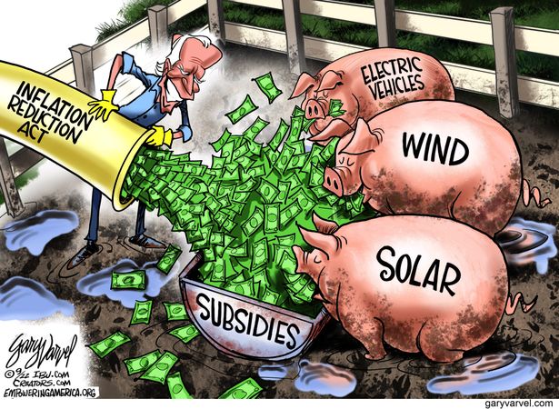
So I like the technology parts of the IRA I do not like the subsidies for wind and solar. One of the things you didn’t mention was I was Chief scientist for BP the oil company for five years. So I learned the energy industry. I never had to make any money in it, but I helped to strategize and kind of systematize thinking for them. So I know from the inside about subsidies to solar and wind. Everybody thinks that’s a solution, but of course wind and solar are intermittent sources of electricity: solar obviously doesn’t produce at night or when it’s cloudy, wind does not produce when the wind doesn’t blow. If you’re going to build a grid that’s entirely wind and solar you better have some way of filling in the times when they’re not producing.
Now if it’s only eight hours or 12 hours you’re trying to fill in, not so hard you can build batteries and so on. But if you need to fill in a couple weeks such as times in Europe, Texas and California when the wind has become still and the solar is clouded out. So you need something else right and that might be batteries although I think that’s unlikely. Gas with carbon capture or nuclear is going to be at least as capable as the wind and solar and since the wind and solar feeds are the cheapest the backup system is going to be more expensive, so you wind up running two parallel systems making electricity at least twice as expensive.

So I say that wind and solar can be an ornament on the real electrical system
but they can never be the backbone of the system.
Let me explain the biggest problem in trying to reduce emissions is not the one and a half billion people in the developed world; it’s the six and a half billion people who don’t have enough energy. And you’re telling them that because of some vague distant threat that we in the developed world are worried about, that they’re going to have to pay more for energy or get more less reliable sources. They should be able to make their own choices about whether they’re willing to tolerate whatever threat there might be from the climate versus having round-the-clock lighting, having adequate Refrigeration, having transportation and so on. Millions of people in India, six and a half billion people worldwide right absolutely they’re energy starved.

Three billion people on the planet of the 8 billion use less electricity every year than the average U.S refrigerator. So first fix that problem, which is existential and immediate and solvable, and then we can talk about some vague climate thing that might happen 50 years from now.
But scientists must tell the truth, absolutely completely lay it all out,
and we’re not getting that out of the scientific establishment.
PR: Unsettled has been out for more than two years now how have your colleagues responded?
SK: Many colleagues who are not climate scientists say thanks for writing the book it gives me a framework to think about these things and points me to some of the problems that we’re seeing in the popular discussion. I got some rather awful reviews from mainstream climate scientists which disappointed me. Not because they found anything wrong in the book, they didn’t. But the quality of the discussion, the ad hominem attacks, the putting words in my mouth and so on, that wasn’t so good. Their argument was, Steve Koonin you’re one of us ; you shouldn’t be saying this. It may be true but you shouldn’t be saying it. Steve how could you?
First of all I’ve been involved in science advice in other aspects of public policy particularly National Defense together with some Stanford former colleagues now passed on. And I was taught that you tell the whole truth and you let the politicians make the value judgments and the cost Effectiveness trade-offs. My sense of that balance is no better than anybody else’s, but I can bring to the table the scientific facts. If you trust democracy, you trust people to elect politicians who can over time make a mistake here, they’ll make a mistake there.
But over time you trust them. Now there are colleagues who say: No don’t tell them the truth we can’t trust them to make the right decision. That’s fundamentally what’s going on. I know scientists who know better than everybody else, and you know it’s even worse because these are scientists in the developed world. And if you ask the scientists in Nigeria or India and so on, you get a very different values calculus, that the primary concern is getting enough energy for folks.

PR: According to a Harris poll in January 2022 a little over a year year and a half ago now 84% of teenagers in the United States agree with both of the two following statements. they agree with:
♦ Climate change will impact everyone in my generation through Global political instability.
♦ If we don’t address climate change today it will be too late for future Generations making some parts of the planet unlivable.
John Kerry, Al Gore, Greta Thunberg and on and on, and countless voices warning that climate change represents a genuine danger to life on the planet. And now millions of Young Americans are really scared. Surely this has some role to play in what we see the the suicidal ideation and the increasing unhappiness.

SK: I’m sure there are all kinds of social factors but surely this is part of what’s going on. There are two immoralities here. One is the immoral treatment of the developing World which we talked about. The other immorality is scaring the bejesus out of the younger generation. And it’s doubly dangerous because it’s mostly in the west and not in China or India. I’ve tried. I go out and talk in universities and of course the audiences I talk to tend to be quantitative and factually driven. So the minds get opened up if the eyes get opened up.
I think in the U.S the problem will eventually solve itself because the route we are headed down is starting to impact people’s daily lives. Electricity is getting more expensive, you won’t be able to buy an internal combustion car in 10 or 15 years. If you’re here in California, people are going to say wait a second, as they already are in Europe, in UK , Germany, France. And I think there will be a falling down to Earth of all of this at some point and we will get more sensible.
PR: Let’s say your audience now is not a colleague of yours but is an 18 to 24 year old American pretty bright, maybe in college maybe not, but bright. Reads newspapers or at least reads them online. Speaking to that person speaking to an American kid or young adult: Do you need, do they need to be scared?
SK: No absolutely not. I would quote the 1900 to now flourishing as an example. And I would say, you probably believe that hurricanes are getting worse, and then point them to the IPCC line. And say you know you were misinformed about that by the media, don’t you think that there are other things about which you’ve been misinformed. You can read the book and find out many of them, and then go ask your climate friends how come it says one thing in the IPCC report but you’re telling me something else.